STRESS-STRAIN CURVES
David Roylance
Department of Materials Science and Engineering Massachusetts Institute of Technology
Cambridge, MA 02139 August 23, 2001
Introduction
Stress-strain curves are an extremely important graphical measure of a material’s mechanical properties, and all students of Mechanics of Materials will encounter them often. However, they are not without some subtlety, especially in the case of ductile materials that can undergo sub-stantial geometrical change during testing. This module will provide an introductory discussion of several points needed to interpret these curves, and in doing so will also provide a preliminary overview of several aspects of a material’s mechanical properties. However, this module will not attempt to survey the broad range of stress-strain curves exhibited by modern engineering materials (the atlas by Boyer cited in the References section can be consulted for this). Several of the topics mentioned here — especially yield and fracture — will appear with more detail in later modules.
“Engineering” Stress-Strain Curves
Perhaps the most important test of a material’s mechanical response is the tensile test1, in which one end of a rod or wire specimen is clamped in a loading frame and the other subjected to a controlled displacement δ (see Fig. 1). A transducer connected in series with the specimen provides an electronic reading of the loadP(δ) corresponding to the displacement. Alternatively, modern servo-controlled testing machines permit using load rather than displacement as the controlled variable, in which case the displacement δ(P) would be monitored as a function of load.
The engineering measures of stress and strain, denoted in this module as σe and e respec-tively, are determined from the measured the load and deflection using the original specimen cross-sectional areaA0 and lengthL0 as
σe= AP
0, e =
δ
L0 (1)
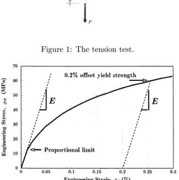
When the stress σe is plotted against the strain e, an engineering stress-strain curve such as that shown in Fig. 2 is obtained.
1Stress-strain testing, as well as almost all experimental procedures in mechanics of materials, is detailed by
standards-setting organizations, notably the American Society for Testing and Materials (ASTM). Tensile testing of metals is prescribed by ASTM Test E8, plastics by ASTM D638, and composite materials by ASTM D3039.
Figure 1: The tension test.
Figure 2: Low-strain region of the engineering stress-strain curve for annealed polycrystaline copper; this curve is typical of that of many ductile metals.
In the early (low strain) portion of the curve, many materials obey Hooke’s law to a reason-able approximation, so that stress is proportional to strain with the constant of proportionality being the modulus of elasticity or Young’s modulus, denotedE:
σe=Ee (2)
As strain is increased, many materials eventually deviate from this linear proportionality, the point of departure being termed the proportional limit. This nonlinearity is usually as-sociated with stress-induced “plastic” flow in the specimen. Here the material is undergoing a rearrangement of its internal molecular or microscopic structure, in which atoms are being moved to new equilibrium positions. This plasticity requires a mechanism for molecular mo-bility, which in crystalline materials can arise from dislocation motion (discussed further in a later module.) Materials lacking this mobility, for instance by having internal microstructures that block dislocation motion, are usually brittle rather than ductile. The stress-strain curve for brittle materials are typically linear over their full range of strain, eventually terminating in fracture without appreciable plastic flow.
Note in Fig. 2 that the stress needed to increase the strain beyond the proportional limit in a ductile material continues to rise beyond the proportional limit; the material requires an ever-increasing stress to continue straining, a mechanism termedstrain hardening.
when the load is removed, so the proportional limit is often the same as or at least close to the materials’s elastic limit. Elasticity is the property of complete and immediate recovery from an imposed displacement on release of the load, and the elastic limit is the value of stress at which the material experiences a permanent residual strain that is not lost on unloading. The residual strain induced by a given stress can be determined by drawing an unloading line from the highest point reached on the se - ee curve at that stress back to the strain axis, drawn with a slope equal to that of the initial elastic loading line. This is done because the material unloads elastically, there being no force driving the molecular structure back to its original position.
A closely related term is the yield stress, denoted σY in these modules; this is the stress needed to induce plastic deformation in the specimen. Since it is often difficult to pinpoint the exact stress at which plastic deformation begins, the yield stress is often taken to be the stress needed to induce a specified amount of permanent strain, typically 0.2%. The construction used to find this “offset yield stress” is shown in Fig. 2, in which a line of slopeE is drawn from the strain axis ate= 0.2%; this is the unloading line that would result in the specified permanent strain. The stress at the point of intersection with theσe−e curve is the offset yield stress.
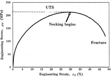
Figure 3 shows the engineering stress-strain curve for copper with an enlarged scale, now showing strains from zero up to specimen fracture. Here it appears that the rate of strain hardening2 diminishes up to a point labeled UTS, for Ultimate Tensile Strength (denotedσf in these modules). Beyond that point, the material appears to strain soften, so that each increment of additional strain requires a smaller stress.
Figure 3: Full engineering stress-strain curve for annealed polycrystalline copper. The apparent change from strain hardening to strain softening is an artifact of the plotting procedure, however, as is the maximum observed in the curve at the UTS. Beyond the yield point, molecular flow causes a substantial reduction in the specimen cross-sectional area A, so the true stress σt = P/A actually borne by the material is larger than the engineering stress computed from the original cross-sectional area (σe = P/A0). The load must equal the true stress times the actual area (P =σtA), and as long as strain hardening can increaseσt enough to compensate for the reduced areaA, the load and therefore the engineering stress will continue to rise as the strain increases. Eventually, however, the decrease in area due to flow becomes larger than the increase in true stress due to strain hardening, and the load begins to fall. This
is a geometrical effect, and if the true stress rather than the engineering stress were plotted no maximum would be observed in the curve.
At the UTS the differential of the load P is zero, giving an analytical relation between the true stress and the area at necking:
P =σtA→dP = 0 =σtdA+Adσt→ −dAA = dσσt t
(3) The last expression states that the load and therefore the engineering stress will reach a maxi-mum as a function of strain when the fractional decrease in area becomes equal to the fractional increase in true stress.
Even though the UTS is perhaps the materials property most commonly reported in tensile tests, it is not a direct measure of the material due to the influence of geometry as discussed above, and should be used with caution. The yield stressσY is usually preferred to the UTS in designing with ductile metals, although the UTS is a valid design criterion for brittle materials that do not exhibit these flow-induced reductions in cross-sectional area.
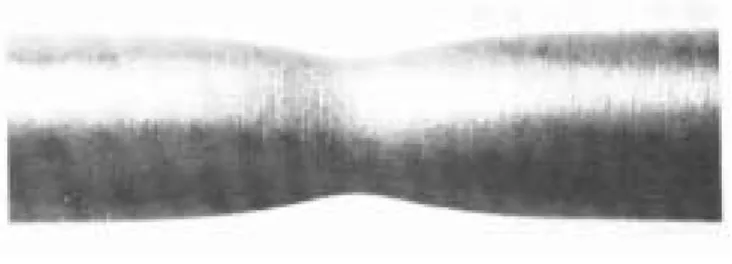
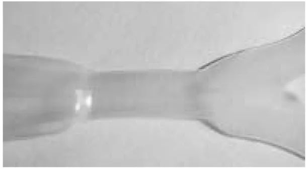
The true stress is not quite uniform throughout the specimen, and there will always be some location - perhaps a nick or some other defect at the surface - where the local stress is maximum. Once the maximum in the engineering curve has been reached, the localized flow at this site cannot be compensated by further strain hardening, so the area there is reduced further. This increases the local stress even more, which accelerates the flow further. This localized and increasing flow soon leads to a “neck” in the gage length of the specimen such as that seen in Fig. 4.
Figure 4: Necking in a tensile specimen.
Until the neck forms, the deformation is essentially uniform throughout the specimen, but after necking all subsequent deformation takes place in the neck. The neck becomes smaller and smaller, local true stress increasing all the time, until the specimen fails. This will be the failure mode for most ductile metals. As the neck shrinks, the nonuniform geometry there alters the uniaxial stress state to a complex one involving shear components as well as normal stresses. The specimen often fails finally with a “cup and cone” geometry as seen in Fig. 5, in which the outer regions fail in shear and the interior in tension. When the specimen fractures, the engineering strain at break — denoted f — will include the deformation in the necked region and the unnecked region together. Since the true strain in the neck is larger than that in the unnecked material, the value off will depend on the fraction of the gage length that has necked. Therefore,f is a function of the specimen geometry as well as the material, and thus is only a
crude measure of material ductility.
Figure 5: Cup-and-cone fracture in a ductile metal.
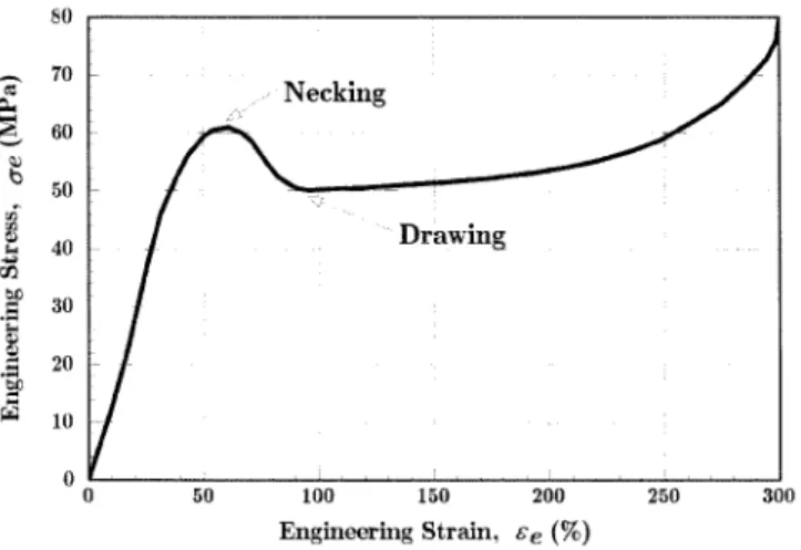
Figure 6 shows the engineering stress-strain curve for a semicrystalline thermoplastic. The response of this material is similar to that of copper seen in Fig. 3, in that it shows a proportional limit followed by a maximum in the curve at which necking takes place. (It is common to term this maximum as the yield stress in plastics, although plastic flow has actually begun at earlier strains.)
Figure 6: Stress-strain curve for polyamide (nylon) thermoplastic.
The polymer, however, differs dramatically from copper in that the neck does not continue shrinking until the specimen fails. Rather, the material in the neck stretches only to a “natural draw ratio” which is a function of temperature and specimen processing, beyond which the material in the neck stops stretching and new material at the neck shoulders necks down. The neck then propagates until it spans the full gage length of the specimen, a process calleddrawing. This process can be observed without the need for a testing machine, by stretching a polyethylene “six-pack holder,” as seen in Fig. 7.
Not all polymers are able to sustain this drawing process. As will be discussed in the next section, it occurs when the necking process produces a strengthened microstructure whose breaking load is greater than that needed to induce necking in the untransformed material just outside the neck.
Figure 7: Necking and drawing in a 6-pack holder.
“True” Stress-Strain Curves
As discussed in the previous section, the engineering stress-strain curve must be interpreted with caution beyond the elastic limit, since the specimen dimensions experience substantial change from their original values. Using the true stress σt = P/A rather than the engineering stress
σe =P/A0 can give a more direct measure of the material’s response in the plastic flow range. A measure of strain often used in conjunction with the true stress takes the increment of strain to be the incremental increase in displacementdLdivided by the current lengthL:
dt= dLl →t= L l0 1 LdL= ln L L0 (4)
This is called the “true” or “logarithmic” strain.
During yield and the plastic-flow regime following yield, the material flows with negligible change in volume; increases in length are offset by decreases in cross-sectional area. Prior to necking, when the strain is still uniform along the specimen length, this volume constraint can be written: dV = 0→AL=A0L0→ LL 0 = A A 0 (5)
The ratioL/L0is theextension ratio,denoted asλ. Using these relations, it is easy to develop relations between true and engineering measures of tensile stress and strain (see Prob. 2):
σt=σe(1 +e) =σeλ, t= ln (1 +e) = lnλ (6) These equations can be used to derive the true stress-strain curve from the engineering curve, up to the strain at which necking begins. Figure 8 is a replot of Fig. 3, with the true stress-strain curve computed by this procedure added for comparison.
Beyond necking, the strain is nonuniform in the gage length and to compute the true stress-strain curve for greater engineering stress-strains would not be meaningful. However, a complete true stress-strain curve could be drawn if the neck area were monitored throughout the tensile test, since for logarithmic strain we have
L L0 = A A 0→ t= lnLL 0 = ln A A 0 (7)
Ductile metals often have true stress-strain relations that can be described by a simple power-law relation of the form:
Figure 8: Comparison of engineering and true stress-strain curves for copper. An arrow indicates the position on the “true” curve of the UTS on the engineering curve.
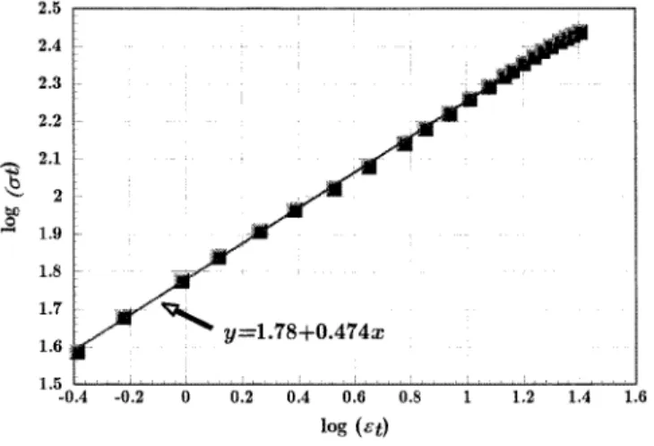
σt=Ant →logσt= logA+nlogt (8) Figure 9 is a log-log plot of the true stress-strain data3 for copper from Fig. 8 that demonstrates this relation. Here the parametern= 0.474 is called thestrain hardening parameter, useful as a measure of the resistance to necking. Ductile metals at room temperature usually exhibit values ofn from 0.02 to 0.5.
Figure 9: Power-law representation of the plastic stress-strain relation for copper. A graphical method known as the “Consid`ere construction” uses a form of the true stress-strain curve to quantify the differences in necking and drawing from material to material. This method replots the tensile stress-strain curve with true stress σt as the ordinate and extension ratio λ= L/L0 as the abscissa. From Eqn. 6, the engineering stress σe corresponding to any
3Here percent strain was used for
t; this produces the same value fornbut a differentA than if full rather than percentage values were used.
value of true stressσtis slope of a secant line drawn from origin (λ= 0, notλ= 1) to intersect theσt−λcurve atσt.
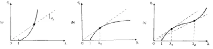
Figure 10: Consid`ere construction. (a) True stress-strain curve with no tangents - no necking or drawing. (b) One tangent - necking but not drawing. (c) Two tangents - necking and drawing. Among the many possible shapes the true stress-strain curves could assume, let us consider the concave up, concave down, and sigmoidal shapes shown in Fig. 10. These differ in the number of tangent points that can be found for the secant line, and produce the following yield characteristics:
(a) No tangents: Here the curve is always concave upward as in part (a) of Fig. 10, so the slope of the secant line rises continuously. Therefore the engineering stress rises as well, without showing a yield drop. Eventually fracture intercedes, so a true stress-strain curve of this shape identifies a material that fractures before it yields.
(b) One tangent: The curve is concave downward as in part (b) of Fig. 10, so a secant line reaches a tangent point at λ = λY. The slope of the secant line, and therefore the engineering stress as well, begins to fall at this point. This is then the yield stressσY seen as a maximum in stress on a conventional stress-strain curve, andλY is the extension ratio at yield. The yielding process begins at some adventitious location in the gage length of the specimen, and continues at that location rather than being initiated elsewhere because the secant modulus has been reduced at the first location. The specimen is now flowing at a single location with decreasing resistance, leading eventually to failure. Ductile metals such as aluminum fail in this way, showing a marked reduction in cross sectional area at the position of yield and eventual fracture.
(c) Two tangents: For sigmoidal stress-strain curves as in part (c) of Fig. 10, the engineering stress begins to fall at an extension rationλY, but then rises again atλd. As in the previous one-tangent case, material begins to yield at a single position when λ = λY, producing a neck that in turn implies a nonuniform distribution of strain along the gage length. Material at the neck location then stretches toλd, after which the engineering stress there would have to rise to stretch it further. But this stress is greater than that needed to stretch material at the edge of the neck from λY to λd, so material already in the neck stops stretching and the neck propagates outward from the initial yield location. Only material within the neck shoulders is being stretched during propagation, with material inside the necked-down region holding constant atλd, the material’s “natural draw ratio,” and material outside holding atλY. When all the material has been drawn into the necked region, the stress begins to rise uniformly in the specimen until eventually fracture occurs. The increase in strain hardening rate needed to sustain the drawing process in semicrys-talline polymers arises from a dramatic transformation in the material’s microstructure. These materials are initially “spherulitic,” containing flat lamellar crystalline plates, perhaps 10 nm
thick, arranged radially outward in a spherical domain. As the induced strain increases, these spherulites are first deformed in the straining direction. As the strain increases further, the spherulites are broken apart and the lamellar fragments rearranged with a dominantly axial molecular orientation to become what is known as the fibrillar microstructure. With the strong covalent bonds now dominantly lined up in the load-bearing direction, the material exhibits markedly greater strengths and stiffnesses — by perhaps an order of magnitude — than in the original material. This structure requires a much higher strain hardening rate for increased strain, causing the upturn and second tangent in the true stress-strain curve.
Strain energy
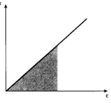
The area under the σe−e curve up to a given value of strain is the total mechanical energy per unit volume consumed by the material in straining it to that value. This is easily shown as follows: U∗ = 1 V P dL= L 0 P A0 dL L0 = 0 σ d (9)
In the absence of molecular slip and other mechanisms for energy dissipation, this mechanical energy is stored reversibly within the material as strain energy. When the stresses are low enough that the material remains in the elastic range, the strain energy is just the triangular area in Fig. 11:
Figure 11: Strain energy = area under stress-strain curve.
Note that the strain energy increases quadratically with the stress or strain; i.e. that as the strain increases the energy stored by a given increment of additional strain grows as the square of the strain. This has important consequences, one example being that an archery bow cannot be simply a curved piece of wood to work well. A real bow is initially straight, then bent when it is strung; this stores substantial strain energy in it. When it is bent further on drawing the arrow back, the energy available to throw the arrow is very much greater than if the bow were simply carved in a curved shape without actually bending it.
Figure 12 shows schematically the amount of strain energy available for two equal increments of strain ∆, applied at different levels of existing strain.
The area up to the yield point is termed themodulus of resilience, and the total area up to fracture is termed themodulus of toughness; these are shown in Fig. 13. The term “modulus” is used because the units of strain energy per unit volume are N-m/m3 or N/m2, which are the same as stress or modulus of elasticity. The term “resilience” alludes to the concept that up to the point of yielding, the material is unaffected by the applied stress and upon unloading
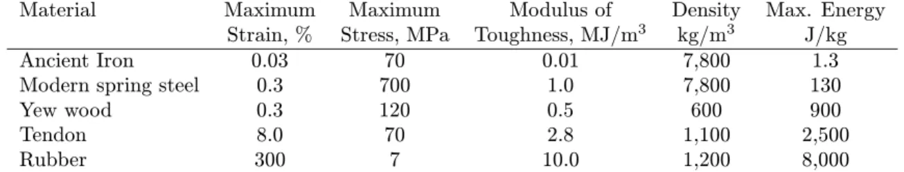
Figure 12: Energy associated with increments of strain Table 1: Energy absorption of various materials.
Material Maximum Maximum Modulus of Density Max. Energy
Strain, % Stress, MPa Toughness, MJ/m3 kg/m3 J/kg
Ancient Iron 0.03 70 0.01 7,800 1.3
Modern spring steel 0.3 700 1.0 7,800 130
Yew wood 0.3 120 0.5 600 900
Tendon 8.0 70 2.8 1,100 2,500
Rubber 300 7 10.0 1,200 8,000
will return to its original shape. But when the strain exceeds the yield point, the material is deformed irreversibly, so that some residual strain will persist even after unloading. The modulus of resilience is then the quantity of energy the material can absorb without suffering damage. Similarly, the modulus of toughness is the energy needed to completely fracture the material. Materials showing good impact resistance are generally those with high moduli of toughness.
Figure 13: Moduli of resilience and toughness.
Table 14 lists energy absorption values for a number of common materials. Note that natural and polymeric materials can provide extremely high energy absorption per unit weight.
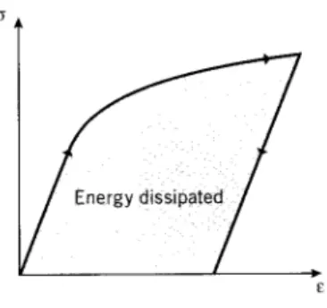
During loading, the area under the stress-strain curve is the strain energy per unit volume absorbed by the material. Conversely, the area under the unloading curve is the energy released by the material. In the elastic range, these areas are equal and no net energy is absorbed. But
if the material is loaded into the plastic range as shown in Fig. 14, the energy absorbed exceeds the energy released and the difference is dissipated as heat.
Figure 14: Energy loss = area under stress-strain loop.
Compression
The above discussion is concerned primarily with simple tension, i.e. uniaxial loading that increases the interatomic spacing. However, as long as the loads are sufficiently small (stresses less than the proportional limit), in many materials the relations outlined above apply equally well if loads are placed so as to put the specimen in compression rather than tension. The expression for deformation and a given loadδ=P L/AE applies just as in tension, with negative values forδ and P indicating compression. Further, the modulus E is the same in tension and compression to a good approximation, and the stress-strain curve simply extends as a straight line into the third quadrant as shown in Fig. 15.
Figure 15: Stress-strain curve in tension and compression.
There are some practical difficulties in performing stress-strain tests in compression. If excessively large loads are mistakenly applied in a tensile test, perhaps by wrong settings on the testing machine, the specimen simply breaks and the test must be repeated with a new specimen. But in compression, a mistake can easily damage the load cell or other sensitive components, since even after specimen failure the loads are not necessarily relieved.
Specimens loaded cyclically so as to alternate between tension and compression can exhibit hysteresis loops if the loads are high enough to induce plastic flow (stresses above the yield stress). The enclosed area in the loop seen in Fig. 16 is the strain energy per unit volume released as heat in each loading cycle. This is the well-known tendency of a wire that is being
bent back and forth to become quite hot at the region of plastic bending. The temperature of the specimen will rise according to the magnitude of this internal heat generation and the rate at which the heat can be removed by conduction within the material and convection from the specimen surface.
Figure 16: Hysteresis loop.
Specimen failure by cracking is inhibited in compression, since cracks will be closed up rather than opened by the stress state. A number of important materials are much stronger in com-pression than in tension for this reason. Concrete, for example, has good compressive strength and so finds extensive use in construction in which the dominant stresses are compressive. But it has essentially no strength in tension, as cracks in sidewalks and building foundations attest: tensile stresses appear as these structures settle, and cracks begin at very low tensile strain in unreinforced concrete.
References
1. Boyer, H.F.,Atlas of Stress-Strain Curves, ASM International, Metals Park, Ohio, 1987. 2. Courtney, T.H.,Mechanical Behavior of Materials, McGraw-Hill, New York, 1990. 3. Hayden, H.W., W.G. Moffatt and J. Wulff, The Structure and Properties of Materials:
Vol. III Mechanical Behavior,Wiley, New York, 1965.
Problems
1. The figure below shows the engineering stress-strain curve for pure polycrystalline alu-minum; the numerical data for this figure are in the file aluminum.txt, which can be imported into a spreadsheet or other analysis software. For this material, determine (a) Young’s modulus, (b) the 0.2% offset yield strength, (c) the Ultimate Tensile Strength (UTS), (d) the modulus of resilience, and (e) the modulus of toughness.
2. Develop the relations given in Eqn. 6:
Prob. 1
3. Using the relations of Eqn. 6, plot the true stress-strain curve for aluminum (using data from Prob.1) up to the strain of neck formation.
4. Replot the the results of the previous problem using log-log axes as in Fig. 9 to determine the parameters Aand nin Eqn. 8 for aluminum.
5. Using Eqn. 8 with parameters A = 800 MPa, n = 0.2, plot the engineering stress-strain curve up to a strain ofe = 0.4. Does the material neck? Explain why the curve is or is not valid at strains beyond necking.
6. Using the parameters of the previous problem, use the condition (dσe/de)neck= 0 to show that the engineering strain at necking ise,neck = 0.221.
7. Use a Consid`ere construction (plot σt vs. λ, as in Fig. 10 ) to verify the result of the previous problem.
8. Elastomers (rubber) have stress-strain relations of the form
σe= E3 λ− 1 λ2 ,
where E is the initial modulus. Use the Consid`ere construction to show whether this material will neck, or draw.
9. Show that a power-law material (one obeying Eqn. 8) necks when the true straintbecomes equal to the strain-hardening exponentn.
10. Show that the UTS (engineering stress at incipient necking) for a power-law material (Eqn. 8) is
σf = An n
en
11. Show that the strain energyU = σ dcan be computed using either engineering or true values of stress and strain, with equal result.
12. Show that the strain energy needed to neck a power-law material (Eqn.8) is
U = An
n+1