structure
Jorge Fernández Ruiz* y Blanca Cecilia García Medina*
Fecha de recepción: 16 de mayo de 2002; fecha de aceptación: 4 de febrero de 2003Abstract: We study the relationship of risk aversion and debt maturity structure. In a model in which adverse selection in financial markets creates a role for the use of short-term debt, we allow the possibility of borrowers being risk-averse. This creates a trade-off between reduced expected financing costs and higher risk and allows for the study of the effect of risk aversion on optimal maturity structure. We prove that, as risk aversion increases, so does the percentage of debt that is long-term.
Keywords: risk aversion, debt maturity structure, adverse selection.
Resumen: En este artículo estudiamos la relación entre la aversión al riesgo y la estructura de vencimiento de la deuda. En un modelo en que la selección adversa en los mercados financieros ocasiona que la deuda de corto plazo sea útil, permitimos que los deudores sean aversos al riesgo. Esto crea una tensión entre la reducción de los costos financieros esperados y el aumento en el riesgo, y permite que se analice el efecto de la aversión al riesgo en la estructura óptima de vencimiento de la deuda. Probamos que el porcentaje óptimo de deuda de largo plazo aumenta conforme se incrementa la aversión al riesgo.
Palabras clave: aversión al riesgo, estructura de vencimiento de deuda, selección adversa.
Introduction
T
he importance of understanding debt maturity structure has been recently gaining recognition in the financial economics literature and important progress has been made in its analysis. For instance, Barclay and Smith (1995) emphasize the importance of this issue and provide an empirical examination of the determinants of debt maturity at the firm level. At the country level, recent experiences in Mexico and other developing countries have caused the analysis of international debt problems to move beyond the pure issue of debt size to include more detailed aspects of the financing process including the debt maturity profile.1 In this paper, we add to the literature on debt maturity structure and focus on its relationship with one borrower characteristic that has not hitherto received much attention in the literature, namely, the borrower’s risk aversion.In this paper, we rely on Flannery’s (1986) and Diamond’s (1991, 1993) view on why there is short-term debt. According to this view, short-term debt can help alleviate adverse selection problems in financial markets. To see why, consider a situation in which a firm has better information than its lenders about the project it wants to undertake. Usually, lenders will be able to observe the performance of the firm and learn about it during the life of the project. This will reduce the initial asymmetry of information. The role of short-term debt arises precisely from this fact. Indeed, consider the choice of debt maturity. The natural choice is for debt to mature at the same time at which the project will render its fruits: to match the maturity of the debt with the project it is going to finance. Apparently, a mismatch between the maturity of the project and the debt issued to finance it would only create risks. Yet, some advantages are obtained by financing the project with debt that matures before the project is given time to produce enough cash flows to repay it. The crucial point is simply that lenders learn important information about the firm before enough time has passed to allow for debt repayment. This implies that good borrowers may be willing to borrow debt that matures before it can be repaid out of the project’s cash flows because they know that at this
1 See for instance Cole and Kehoe (1996) for an analysis that emphasizes the importance of
debt maturity structure in the Mexican crisis. Cermeño, Hernández-Trillo and Villagómez (2001) and Sachs, Tornell and Velasco (1996) also deal with the role of public debt structure in the 1994-1995 crisis.
time some new information will be known, showing that they are good. This new information will, in turn, allow them to refinance their debt at better terms.
The advantage of borrowing short-term has to be weighed, however, against the risks it entails. Although good borrowers expect that new information will most likely reveal that they have good projects, this fact can by no means be taken for granted: to the extent that new information will not completely eliminate the asymmetry of information, there is a risk that future news will damage good borrowers. Thus, short-term debt implies a higher risk than long-term debt. In this paper, in contrast to Flannery and Diamond, we allow for firms to be risk averse. This implies that the maturity choice has to balance the benefits of refinancing at terms that allow for a better assessment of the quality of the project against the costs of higher risk. We find the maturity structure that optimally solves this trade-off. Next, we are in a position to analyze the comparative statics of the optimal debt contract. We prove a result that is intuitive: more risk averse firms prefer to issue less short-term debt and more long-term debt than less risk averse firms.
We then extend our analysis to show that our main result extends to more complex settings. In particular, we consider a scenario where there is a risk of a hike in market interest rates during the life of a project, as in Fernández Ruiz (2002). This setting captures a situation where different types of news arrive before the project matures, some of which refer to the firm’s project itself while others do not.
From a formal point of view, our model is closest to Flannery (1986) and Diamond (1991, 1993). Yet, there are important differences. First, in the above papers, borrowers are risk neutral while here the firm is risk averse. Second, and closely related to the previous difference, these papers do not address the issue of the effect of risk aversion on debt maturity structure, which is the focus of our paper. Third, while in these papers there is only one kind of intermediate news, in ours, there are news both about the firm’s project and a variable not directly related to its project-market interest rates. Our paper is also related to Fernández-Ruiz, who studies a model in which a risk averse country finances its development project under asymmetric information, and two types of news —one of which reduces the asymmetry of information— become known before the project matures. But Fernández-Ruiz focuses on the ability of debt contracts to accomplish
the tasks performed by complete contracts. In contrast, in this paper we focus on the role of risk aversion and its effect on debt maturity structure.
I. The Model
In this section we present a model in the spirit of Flannery (1986) and Diamond (1991, 1993). In this model a firm has to raise funds to undertake a project, and has private information about the quality of such a project. An important feature of this model is that during the life of the project, before it matures, lenders receive news about some project’s characteristics which help them reduce the initial asymmetry of information.
A firm needs to raise an amount I to undertake a project. This project will be developed over three periods, t = 0, 1, 2. At t = 0 the firm can borrow the amount I in a competitive credit market if it can provide nonnegative expected returns to lenders. At t = 1, information about the firm’s project arrives. At t = 2 the project is completed and produces cash flow. There are two types of projects, and the firm has private information about the type of project it has. A firm with a good project obtains an income of X > I, while a firm with a bad project obtains X with probability π and 0 otherwise, with π X < I. Thus, under symmetric information, lenders would not finance firms with bad projects. Yet, lenders do not know if a firm has a bad project. At date 0, they assign the firm a probability f of having a good project. Therefore, they assign the firm a probability q = [ f + (1 – f ) π] of obtaining date-two income equal to X.
By observing the performance of the firm, creditors learn something about the firm’s project, which is reflected in the model in the following way: at date t = 1 there are news about the project that reduce the asymmetry of information between the firm and its creditors. These news can be good, s = u (an upgrade of the firm’s rating takes place) or bad, s = d (a downgrade takes place). Good firms receive bad news with probability e, and bad firms with probability r, with e < r.
Creditors update their beliefs about the firm’s type upon observing the realization of s. They do this by applying Bayes’ rule. Let fd ( fu )
be the updated probability —according to Bayes’ rule— that the firm is good given bad (good) news. We have:
(
1 f)
r, fe ef fd − + = (1)( )
( ) (
1 1)(
1)
. 1 r f e f f e fu − − + − − = (2)We can calculate in a similar manner the conditional probability that date-two income will be X given bad (good) news. Let us denote these probabilities by qd ( qu ).
The firm maximizes its expected utility E [u(Y)], where Y is date-two income, net of repayments to creditors, and u’( ) > 0, u”( ) < 0. Capital markets are competitive, and are willing to invest as long as the expected discounted sum of net repayments from the firm equals (or is higher than) 0.
II. Debt maturity structure
The firm can raise the funds to undertake the project by using any combination of two different types of debt, short-term debt and long-term debt, as in Flannery (1986) and Diamond (1991, 1993). The firm can issue short-term debt with nominal value S1 that matures at t=1, after interim news are released, and long-term debt with nominal value D, that comes due after the project is completed at t=2. To repay
S1, the firm needs to come back to the credit market, since at the time
S1 matures the project that has not yet produced any income. Thus, we assume that at t=1 the firm has access again to a competitive credit market in which it can raise funds promising up to (X−D), that
is, the part of the resources that will not be needed to repay long-term debt. Thus, at t=1, the firm issues short-term debt with face value S2 that comes due at t=2. We also assume that S1 and D are such that the firm is always able to raise the necessary funds to repay S1 at t=1. We assume for the moment that the risk-free interest rate is constant throughout the life of the project, and for simplicity we take this interest rate to equal 0. In an extension of the model in the following section we will consider the case in which this interest rate may vary.
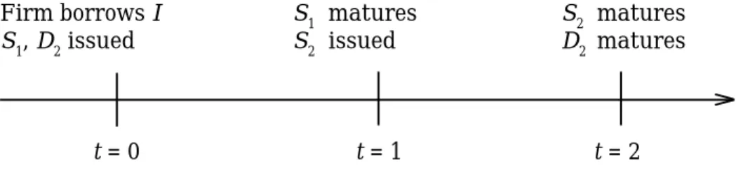
Figure 1 illustrates the timing of the issuance and repayment of the different types of debt.
Figure 1
Firm borrows I S1 matures S2 matures
S1, D2 issued S2 issued D2 matures
t = 0 t = 1 t = 2
We now need to establish several relationships between the different types of debt. First, let us find how much debt the firm must issue at date 1 to borrow the necessary funds to repay S1. This depends on the arrival of good (s = u) or bad (s = d) news about the quality of the project. To borrow S1 at t = 1, the firm must issue debt with face value S2 satisfying:
S2 = S1 / qu if s = u, (3)
S2 = S1 / qd if s = d. (4)
To see why this is so, consider for instance the case s = u, (the explanation for the other case is similar). Since there are good news about the project (s = u), financial markets expect that it will yield X with probability qu. This is the probability with which the firm will
repay the debt S2. Thus, the expected repayment from a debt with face value S2 is qu S2, which must equal the amount borrowed S1.
The firm maximizes its expected utility E[u(Y)], where Y is date-two income net of repayments to creditors, and capital markets are competitive. As in Flannery (1986) and Diamond (1991, 1993) we look for the pooling equilibrium preferred by good quality firms. A good quality firm chooses the amount of short-term debt S1 and long-term debt D so as to solve the following program (we omit the subscript in
( )
− − − + − − θ θ q D S X u e D q S X eu Max d u D S, 1 subject to(
)
[
f f]
S I D +1− π + ≥ .The constraint of this program ensures that lenders will be willing to lend the amount I. Its left-hand side is the repayment they expect to receive from the firm: long-term debt with face value D will be repaid at t = 2 with probability q = [ f +(1- f ) π ], because this is the probability with which date-two cash flow will be X. Short-term debt
S1 will be repaid for sure at t = 1. This repayment has to be at least equal to I for lenders to be willing to lend. Let us now look at the objective function. It is the firm’s expected utility from its date-two income X net of repayments to creditors. These repayments consist of long-term debt with face value D, plus short-term debt with face value
S2. Consider the first term. With probability e there will be bad news about the firm’s project (s = d). In this case, short-debt repayments amount to S2 = S1 / qd, as determined by (4). The explanation for the
other term is similar.
We will consider the family of utility functions with a constant (Arrow-Pratt) measure of absolute risk aversion,
θ = ′ ′′ − = u u x ru( ) .
These utility functions are of the form ), exp( )
(x a b x
uθ = + −θ
where a higher θ is associated with more risk aversion. Notice that
u’( ) > 0, u’’( ) < 0 imply b < 0 and θ> 0.
Let us assume, without any loss in generality, that a=0 and
b= −1, so that the firm chooses the debt structure (S1, D) that solves the following program.
(Program 1) − − θ − − − − − θ − − D q S X e D q S X e Max d u S exp (1 )exp subject to
(
)
[
f f]
S I D + 1− π + ≥ .As is shown in the appendix, the comparative statics of the solution to program (1) lead to the following proposition:
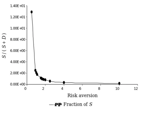
Proposition 1. When the risk-free interest rate is constant along
the life of the project, an increase in the degree of risk aversion θ translates into an optimal financial contract comprising less short-term debt S1 and more long-term debt D.
We illustrate this proposition by showing the optimal debt structure for different degrees of risk aversion, when f = ½, e = ¼, r = ½, π = ½,
I = 1, and X = 2.
III. An extension: risk of change in interest rates
In this section we consider an extension of the above model that considers the arrival of news not related to the project itself during the life of the project, as in Fernández Ruiz (2002). More precisely, there may be a hike in interest rates during the life of the project. So, the model is modified as follows:
At t = 1, information about the firm’s project and about market interest rates arrive. Thus, there are two types of news. First, as in the previous section, there are news about the project that reduce the asymmetry of information between the firm and its creditors. But now there are also news about risk-free interest rates. They may remain constant or increase: the one-period risk-free interest rate (that is, the interest rate on a loan that will be repaid for sure) remains at 0 with probability λ, and increases to i > 0 with probability (1 – λ).
The possibility of a hike in interest rates modifies the relationships between the different types of debt. More precisely, the amount of debt
Figure 2. Fraction of short-term debt as risk aversion varies when
i=0
the firm must issue at date 1 to borrow the necessary funds to repay
S1 depends now not only on the arrival of good (s=u) or bad (s=d) news about the quality of the project, but also on whether the interest rate remains at 0 (n=c), or rises to i > 0 (n=h). To borrow S1 at t=1, the firm must issue debt with face value S2 satisfying:
Table 1. Optimal values of short-term and long-term debt when i=0 as risk aversion varies
Theta Fraction of S S D 10.000 1.27E–01 0.1622 1.1171 4.000 3.38E–01 0.4055 0.7927 2.500 5.69E–01 0.6187 0.4683 2.000 7.63E–01 0.8109 0.2521 1.800 8.72E–01 0.9010 0.1320 1.650 9.77E–01 0.9829 0.0227 1.621 1.00E+00 1.0005 0.0000 1.40E+01 1.20E+01 1.00E+01 8.00E+00 6.00E+00 4.00E+00 2.00E+00 0.00E+00 0 2 4 6 8 10 12 ———• Fraction of S Risk aversion S / ( S + D )
S2 = S1 (1 + i) / qu if s = u, n = h, (5)
S2 = S1 / qu if s = u, n = c, (6)
S2 = S1 (1 + i) / qd if s = d, n = h, (7)
S2 = S1 / qd if s = d, n = c. (8)
To see why this is so, consider for instance the case s = u, n = h (the explanation for the other cases is similar). Since there are good news about the project (s = u), financial markets expect that it will yield X with probability qu. This is the probability with which the firm will
repay the debt S2. Thus, the expected repayment from a debt with face value S2 is quS2. Therefore, short-term debt S2 offers an expected (gross) rate of return of qu S
2 / S1, which must equal the (gross) interest rate 1+ i, from where S2 = S1 (1 + i) / qu follows.
Given these relationships, we will look again for the contract preferred by good quality firms among the pooling equilibrium contracts. The amounts of short-term debt S1 and long-term debt D are thus chosen so as to solve the following program:
− − λ − + − + − λ − − + − − λ + − + − λ − θ θ θ θ D q S X u e D q i S X u e D q S X u e D q i S X u e Max u u d d D S ) 1 ( ) 1 ( ) 1 )( 1 ( ) 1 ( ) 1 ( , subject to
(
)
[
f f]
S[
(
) ( )
i]
I[
(
) ( )
i]
D + 1− π + λ+ 1−λ 1+ ≥ λ+ 1−λ 1+ .Let us interpret this program. As before, the constraint ensures that lenders will be willing to lend the amount I and its left-hand side is the repayment they expect to receive from the firm: long-term debt with face value D will be repaid at t = 2 with probability q = [ f+(1−f )π], because with this probability date-two cash flow will be X. Short-term
debt S1 will be repaid for sure at t = 1, which explains the second term in the left-hand side. The right-hand side is the opportunity cost of I. With respect to the objective function, it is again a good firm’s expected utility from its date-two income X net of repayments to creditors. It has now four terms because there can be four different combinations of date-one news. Let us interpret the first term. With probability e(1− λ) there will be bad news about the firm’s project (s=d) and a hike in interest rates (n=h). In this case, short-debt
repayments amount to S2=S1(1+i) / qd, as determined by (7). The explanation for the other three terms is similar.
When using a utility function with constant absolute risk aversion, the debt structure (S1, D) solves the following program:
(Program 2) − − θ − λ − − − + − θ − λ − − − − − θ − λ − − + − θ − λ − − D q S X e D q i S X e D q S X e D q i S X e Max u u d d S exp ) 1 ( ) 1 ( exp ) 1 )( 1 ( exp ) 1 ( exp ) 1 ( subject to
(
)
[
f f]
S[
(
) ( )
i]
I[
(
) ( )
i]
D + 1− π + λ+ 1−λ 1+ ≥ λ+ 1−λ 1+ .The comparative statics of the solution to program (2) lead (see appendix) to the following proposition:
Proposition 2. When the risk-free interest rate may rise at t = 1,
an increase in the degree of risk aversion θ translates into an optimal financial contract comprising less short-term debt S1 and more long-term debt D.
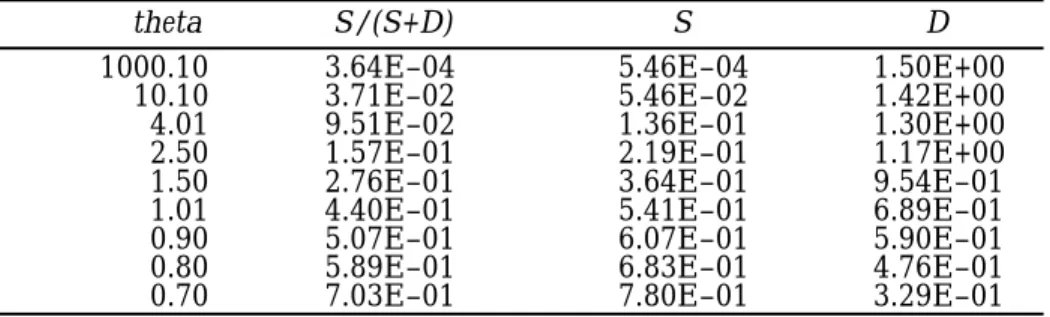
We illustrate this proposition using the same values as in the example after proposition 1, plus λ = ½ and i = ¼.
Table 2. Optimal values of short-term (S) and long-term debt (D) when
i=====¼ as risk aversion varies
theta S/(S+D) S D
1000.10 3.64E–04 5.46E–04 1.50E+00
10.10 3.71E–02 5.46E–02 1.42E+00
4.01 9.51E–02 1.36E–01 1.30E+00
2.50 1.57E–01 2.19E–01 1.17E+00
1.50 2.76E–01 3.64E–01 9.54E–01
1.01 4.40E–01 5.41E–01 6.89E–01
0.90 5.07E–01 6.07E–01 5.90E–01
0.80 5.89E–01 6.83E–01 4.76E–01
0.70 7.03E–01 7.80E–01 3.29E–01
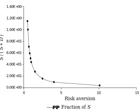
Figure 3 shows the proportion S /(S+D).
IV. Conclusions
We devote this section to summing up our main findings and to comment on two issues not dealt with in our model that deserve attention.
In this paper we have focused on the role of risk aversion on debt maturity structure. We have drawn on the argument made by Flannery (1986) and Diamond (1991, 1993) among others, that adverse selection problems in financial markets can explain a divergence between debt maturity and project maturity, to build a model amenable to study the relationship between risk aversion and debt maturity structure.
The idea leading to the use of short-term debt in the basic model is that good borrowers prefer short-term debt because it allows them to refinance at a time when their performance has shown that they are indeed good. This benefit of short-term debt has to be balanced against the higher risk it creates. We have proved in this basic model the intuitive result that as risk aversion increases so does the proportion of total debt that is long-term.
We have extended the basic model to allow for uncertainty in variables not directly related to the project to be financed. Thus, we have considered a situation in which during the life of a project there are two kind of news. One of these news reduces the asymmetry of information between the borrower and the lender. The other one does not directly relate to the project. We have taken this second variable to be the one-period risk-free interest rate. We have found that in this
Figure 3. Short-term debt as a fraction of total debt as risk aversion
varies when i = ¼
extended setting our previous result continues to hold: More risk averse borrowers find it optimal to contract a higher proportion of long-term debt.
We now deal with two issues not addressed in the model that deserve some comment. The first one calls for an extension of the model that is best understood by considering a situation where the intermediate signal is so bad that both the firm and its lenders know that the project is useless. To deal with this issue, we could extend the model to allow for liquidation. In other words, to allow for the project to be canceled before it matures. Although cancellation of the project before its maturity would come at a cost —a partial loss of the initial investment— it would avoid a worst-case scenario. This has implications for the optimal debt maturity structure, since firm’s liabilities should be designed to make efficient use of future information and this may imply setting the firm’s liabilities so as to make possible canceling the project if the news are sufficiently bad. When comparing the advantages and disadvantages of short-term versus long-term debt,
1.40E+00 1.20E+00 1.00E+00 8.00E+01 6.00E+01 4.00E+01 2.00E+01 0.00E+00 0 5 10 15 ———• Fraction of S Risk aversion S / ( S + D )
it should be noticed that the first one is better equipped to deal with these situations, since it forces the firm to come back to the capital markets before the projects mature. If these markets’ assessment of the quality of the project is negative, the firm will be unable to refinance its debt. This, in turn, will force the firm to liquidate its project and will allow investors to recover some of their initial investment. On the other hand, by using short-term debt we will face the risk of inefficiently liquidating the project. Summing up, adding this extra dimension would both make the model more difficult and enrich the analysis.
The second comment has to do with liquidity issues. The structure of the model does not consider them and one could think of at least two ways in which they could be added. First, there is no liquidity premium present in the equations that describe the relationship between long-term and short-term interest rates. Second, the firm does not face the possibility of a liquidity shock at any point during the life of the project. They are simplifying assumptions that make the model more tractable.
These two issues deserve attention. Yet, by abstracting from them we have been able to isolate one important channel through which risk aversion affects the optimal debt maturity structure.
References
Barclay, M. J. and C. W. Smith Jr. (1995), “The Maturity Structure of Corporate Debt”, Journal of Finance, num. 50, pp. 609-631. Cermeño, R., F. Hernández-Trillo y A. Villagómez (2001), “Regímenes
Cambiantes, Estructura de Deuda y Fragilidad Bancaria en México”, Estudios Económicos, núm. 16.
Cole, H. and T. J. Kehoe (1996), “A self-fulfilling model of Mexico’s 1994-1995 debt crisis”, Journal of International Economics, num. 41, pp. 309-330.
Diamond, D. W. (1991), “Debt Maturity Structure and Liquidity Risk”,
Quarterly Journal of Economics, num. 106, pp. 709-737.
———, “Bank Loan Maturity and Priority when Borrowers can Refinance”, in Mayer, C. and X. Vives, 1993, Capital Markets and
Dornbusch, R. (1989), “Debt Problems and the World Macroeconomy” in Sachs, J., Developing Firm Debt and Economic Performance, The University of Chicago Press, Chicago.
Fernández-Ruiz, Jorge (2002), “Optimal Financial Contracting and Debt Maturity Structure under Adverse Selection”, Estudios
Económicos, núm. 17.
Flannery, M. J. (1986), “Asymmetric Information and Risky Debt Maturity Choice”, Journal of Finance, num. 41, pp. 19-38.
Sachs, J., A. Tornell and A. Velasco (1996), “The Mexican peso crisis: Sudden death or death foretold?”, Journal of International
Economics, num. 41, pp. 265-284.
Appendix
Proof of Proposition 1
It is a particular case of proposition 2, when i = 0.
Proof of Proposition 2
To prove proposition 2, we first solve program (2):
− − θ − λ − − − + − θ − λ − − − − − θ − λ − − + − θ − λ − − D q S X e D q i S X e D q S X e D q i S X e Max u u d d S exp ) 1 ( ) 1 ( exp ) 1 )( 1 ( exp ) 1 ( exp ) 1 ( subject to
(
)
[
f f]
S[
(
) ( )
i]
I[
(
) ( )
i]
D + 1− π + λ+ 1−λ 1+ ≥ λ+ 1−λ 1+ .Notice first that the constraint holds with equality, otherwise we could decrease either S or D, increase the objective function and still satisfy this constraint. Thus, we have that
(
)( )
[
]
(
)( )
, ) 1 ( 1 1 with , ) ( ) ( ) 1 ( 1 1 π − + + λ − + λ = ϕ − ϕ = − π − + + λ − + λ = f f i S I S I f f i Dand program (2) can be written as
. ) ( exp ) 1 ( ) ( ) 1 ( exp ) 1 ( ) 1 ( ) ( exp ) ( ) 1 ( exp ) 1 ( ) ( − −ϕ − θ − λ − − − + −ϕ − θ − λ − − − − −ϕ − θ − λ − − + −ϕ − θ − λ − − = S I q S X e S I q i S X e S I q S X e S I q i S X e S G Max u u d d S We have that
(
)
( )
( )
( )(
)
( )
( )
( )
ϕ − θ − θ θ ϕ − λ − + θ + ϕ − + λ − − + θ ϕ − λ + θ + ϕ − + λ − = ∂ S I X q S q q e q i S q i q e q S q q e q i S q i q e S dG u u u u u u d d d d d d exp exp 1 1 1 exp 1 1 1 exp 1 1 exp 1 1and
(
)
(
)
0. exp 1 ) 1 ( exp ) 1 ( ) 1 ( ) 1 ( ) ( exp 1 ) ( ) 1 ( exp ) 1 ( ) 1 ( 2 2 2 2 2 2 2 2 2 < − −ϕ − θ − ϕ− θ λ − − − −ϕ − θ − ϕ− − θ λ − − − − −ϕ − θ − ϕ− θ λ − − − −ϕ − θ − ϕ− + θ λ − − = S I q S X q e S I q S X q i e S I q S X q e S I q i S X q i e dS G d u u u u d d d dSince this second derivative is negative (each of its four terms is negative), the following first-order condition characterizes an interior maximum: . exp 1 ) 1 ( ) 1 ( exp ) 1 ( ) 1 ( ) 1 ( exp 1 ) 1 ( exp ) 1 ( ) 1 ( 0 θ ϕ − λ − + θ + ϕ − + λ − − + θ ϕ − λ + θ + ϕ − + λ − = u u u u u u d d d d d d q S q q e q i S q i q e q S q q e q i S q i q e
Applying now the implicit function theorem we have, after some simplifications, that θ − = θ ∂ ∂S S