Interest Rate Transmission to Commercial Credit Rates in Austria

(1)

Interest Rate Transmission

to Commercial Credit Rates in Austria

by

Johann Burgstaller *) Working Paper No. 0306

May 2003

D

E

P

A

R

T

M

E

N

T

O

F

E

C

O

N

O

M

I

C

S

J

OOHHAANNNNEESS

K

EEPPLLEERR

U

NNIIVVEERRSSIITTYYOOFF

L

IINNZZ

Johannes Kepler University of Linz Department of Economics Altenberger Strasse 69 A-4040 Linz - Auhof, Austria www.economics.uni-linz.ac.at

*)

(2)

Interest Rate Transmission

to Commercial Credit Rates in Austria

by

Johann Burgstaller†

Johannes Kepler University Linz

May 2003

Abstract: The transmission process from policy-controlled interest rates to bank lending rates deserves reconsideration owing to the implementation of the European Monetary Union (EMU) in 1999. Additional attention to the subject in Austria is due to several large banks which, in 2002, have been charged for not passing on interest rate decreases to their customers. I examine dynamic responses of commercial credit rates to changes in key policy rates and money market rates. Using Austrian data from 1995 to 2002, I show that strength and speed of interest rate transmission depend on whether rates go up or down. With the EMU, asymmetry in interest rate transmission partly declined. The speed of transmission and the relative importance of policy and money market rates for commercial credit rates also were affected.

Keywords: Monetary policy transmission, interest rate pass-through, bank lending rates for commercial credit, European Monetary Union, impulse-response analysis.

JEL classification: E43, E52, G21, G30.

†_{Johannes Kepler University, Department of Economics, Altenberger Str. 69, A-4040 Linz, Austria.} Phone: +43 70 2468 8706, Fax: +43 70 2468 8217, E-mail: johann.burgstaller@jku.at.

I am grateful to Ren´e B¨oheim for valuable comments and helpful discussion. Data are available on request.

(3)

1 Introduction

Banks’ decisions about the yields paid on their assets and liabilities have an impact on the expenditure and investment behavior of deposit holders and borrowers and thus on real economic activity (De Bondt, 2002). So the effectiveness of monetary policy is also about the extent and the speed of retail banks’ interest rates adjustment to changes in policy-controlled interest rates. Bank lending rates to non-financial firms are a key indicator of the cost of short-term external funding in an economy (Borio and Fritz, 1995).

Retail banks may react quickly or slowly to a change in policy-controlled rates. Toolsema et al. (2001) discussed the relevance of asymmetric information, adjustment and switching costs, as well as risk sharing in expaining sluggish responses of bank lending rates. Empirically, the interest rate channel of monetary transmission also has received renewed attention. Different kinds of data and methodologies have been applied, and most authors agree on the following results:

• There is considerable stickiness of retail lending rates in the short term. At the

European level, for example, the proportion of a given market interest rate change that is passed on to short-term commercial lending rates within one month is around 30 % (De Bondt, 2002).

• There are remarkable cross-country differences with respect to the stickiness of the

short-term lending rate. It depends on the stage of financial market development, the degree of financial market openness as well as concentration and competition within the banking sector (Cottarelli and Kourelis, 1994). In Europe, these asymmetries are expected to diminish as integration increases (Mojon, 2000).

• The average speed for retail bank interest rates to fully adjust to market interest rate

changes is typically between 3 and 10 months (De Bondt, 2002). The perception that the implementation of the European Monetary Union (EMU) will speed up the pass-through is expressed e.g. by Mojon (2000).

• The final pass-through of market to retail bank interest rates is typically complete

or even well above 100 %, as in the case of loans to enterprises of up to one year. Overshooting may, among other factors, be explained by asymmetric information costs without credit rationing. If banks increase their lending rates exactly one-for-one with market interest rates they will attract a more risky class of borrowers. Consequently, banks have to increase the lending rate premium charged (De Bondt, 2002).

In contrast to e.g. Weth (2002), using panel data from a bank survey, I will examine aggregate relationships between time series of policy-controlled interest rates and the bank lending rate on short-term commercial loans. Thereby, I will focus on the following four aspects.

First, the response of lending rates may depend on whether or not policy-controlled rates are rising. If credit demand is inelastic in the short term, revenue for the bank is temporarily foregone when rates are lowered but gained when they are raised (see Borio and Fritz, 1995, also for additional explanations). So the pass-through of refinancing cost changes on lending rates may be delayed in periods of falling interest rates. However,

(4)

Borio and Fritz (1995) find no evidence for this kind of asymmetry, whereas Sander and Kleimeier (2002) do for a few European countries.

Second, money market rates might have become less noisy and volatile since the implementation of the European Monetary Union compared to the individual countries before. If this is the case, it would have become easier for banks to identify permanent changes in interest rates (Cottarelli and Kourelis, 1995) which should speed up the interest rate transmission process (Mojon, 2000).

Third, results for Austria are scarce and conflicting. A study of the Bank for Inter-national Settlements from 1994 reports a long-term pass-through of a change in the money market rate on the short-term commercial lending rate of 68 % for the period from 1984 to 1994 (cited in De Bondt, 2002, Table 1). Using data from 1995 to 2000, Donnay and Degryse (2001, Table 3) estimate that 18 % of a change in the money market rate are dis-seminated after 12 months. This appears to be low, although there are Austrian specifics that could account for such a result. Loans represent by far the most important source for external funding of Austrian firms and this dependance might delay transmission if interest rates go down. Additionally, the Austrian banking sector is dominated by credit cooperatives and savings banks being not primarily interested in short-term profits. Their goal is to ensure a stable value of their assets over the long term and to provide constant credit to their clients. Close relationship banking has the additional advantage of reduc-ing asymmetric information (Braumann, 2002). Intertemporal interest-rate smoothreduc-ing is likely to occur and banks which are heavily involved in long-term business with non-banks adjust their lending rates comparatively slowly (Weth, 2002). The Austrian interest rate transmission process obtained further prominence when, in 2002, the EU Commission convicted seven large Austrian banks for not passing on interest rate decreases to their

customers for several times and imposed a fine on them (approx. 124 million Euro)1_.

Fourth, the methodological approach is slightly different from the one used in almost all other time-series applications. The structural model is less restrictive than the bivariate vector autoregression which often is applied. Furthermore, I do not use an error-correction model right from the beginning as I presume interest rates to be near-integrated time series. Therefore, cointegration relations between them might not be present and an error-correction model might not be the most proper approach.

2 Data and methodological framework

I use Austrian data on several interest rates to investigate transmission dynamics: the rate on refinancing operations controlled by the Central Bank, the 3-month interbank (money market) rate, the interest rate on newly granted short-term loans to private enterprises, and the secondary market return on bonds issued by private non-banking institutions. I will refer to these nominal interest rates as policy, interbank and lending rate as well as bond yield in the following. Additional determinants of interest rate movements, the inflation rate and commercial credit growth, complete the data set. The sample starts in March 1995 and ends in December 2002. The appendix provides a more detailed

1_{The “interest rate cartel” (also called “Lombard-Club”) was in place between 1995 and 1998. The banks} involved have argued that they did agree on delays in the pass-through of key interest rate changes, but that none of them sticked to the arrangements.

(5)

description of all the monthly time series. Table 1 presents summary statistics and Figure 1 graphs the policy, the interbank and the lending rate. It becomes evident that the policy and the interbank rate are slightly more volatile after 1998. The spread between them and the bank lending rate narrowed in time as the latter experienced a strong movement downwards in the late 1990s.

As can be seen from the selection of the time series, I allow for both a money market and an administered policy rate in determining the lending rate. The money market rate is mostly seen as the key opportunity cost of the lending decision as it represents the cost of funds or the revenue foregone by extending a loan (Borio and Fritz, 1995). The choice of money market rates to represent monetary policy is motivated by the discontinuity and inaccuracy in policy rate series as the instruments of monetary policy may change during the sample period. Moreover, most of the time, policy is conducted by means of a combination of instruments that would be poorly represented by the sole policy rate. Therefore, the money market rate seems to be the most appropriate measure of monetary policy since it is most correlated with Central Bank policies as a whole (Donnay and Degryse, 2001). The arguments in favor of additionally considering the refinancing operations interest rate are that it can be used to underline the persistence of a specific policy move and thus helps to crystallize expectations about future interest rates. When money market rates are particularly volatile, it may be a better indicator of their persistent, rather than purely transitory, movements (Borio and Fritz, 1995).

None of the series contains seasonal unit roots according to HEGY tests for monthly time series (Franses and Hobijn, 1997), but seasonal dummies seem to be needed to adequately model commercial credit growth. The unit root tests applied are Augmented Dickey-Fuller (Dickey and Fuller, 1979), KPSS (Kwiatowski et al., 1992) and ERS (Elliott et al., 1996) tests. Test results suggest that none of the time series is integrated of an order higher than one. As univariate unit root tests often report different results on whether a series is stationary or integrated of order one and most of the tests have severe shortcomings (low power, above all), I will test for stationarity in the multivariate context later on.

I treat all selected variables as endogenous and assume that their data-generating process can be reasonably well approximated by a finite vector autoregression (VAR) of

orderp(see e.g. Hamilton, 1994, chapter 11 or, for a short but comprehensive discussion,

L¨utkepohl, 1999). The structural VAR for a vector X of n random variables is given by

B0Xt=µs+ p X

i=1

BiXt−i+CZ+²t, (1)

where B0 is the matrix of contemporaneous relations between the variables and the

re-maining B’s and C are (n×n) parameter matrices. The vector Z may contain seasonal

dummies, exogenous variables or a linear time trend. The structural errors²t are assumed

to be instantaneously uncorrelated. Multiplying (1) by B₀−1 leads to the reduced form of

the VAR Xt=µ+ p X i=1 ΦiXt−i+DZ+et, (2)

(6)

where the disturbance term et is an independent white noise process, et ∼ N(0,Σ). The reduced-form errors are contemporaneously correlated, so their covariance matrix Σ is a non-diagonal matrix (which also is non-singular, positive-definite and time-invariant). The vector error-correction representation (VEC), omitting the term for seasonal dummies and exogenous variables, is

∆Xt =µ+ ΠXt−1+

p−1

X i=1

Γi∆Xt−i+et, (3)

which is to be used with cointegration tests and contains only stationary terms if none of the variables is integrated of an order higher than one. If Π has reduced rank, there exists

a decomposition Π = αβ0 _with _α _and _β _{being (}_n_×_r_{) matrices. The columns of}_β _{are to}

be interpreted as stable long-term (cointegrating) relations between the non-differenced

series andβ0_X

t−1 is called the equilibrium error. The Γ’s are (n×n) parameter matrices.

3 VAR order selection and cointegration tests

For VAR lag order selection I apply several procedures. The prespecified maximum is 6 lags. Sequential LR tests suggest either 6 or 2 lags. The Akaike Information criterion favors 6 lags, the Hannan-Quinn and the Schwarz criterion suggest either 1 or 6 as, with increasing order, their respective values exhibit a hump shape. LM-type autocorrelation tests based on the full reduced-form residual vectors (see Johansen, 1995, p. 22) and multivariate normality tests (Mardia, 1980) suggest “well-behaved” residuals for a lag order of 2 or higher. I chose the VAR order to be equal to 2.

With cointegration tests, I search for linear combinations of the variables that are stationary. Because I presume that some of the series might be trend-stationary, I allow for a linear time trend that is restricted to lie within the cointegration space. So, in fact,

∆Xt =µ+α(β0Xt−1+δ1+δ2t) +

p−1

X i=1

Γi∆Xt−i+et (4)

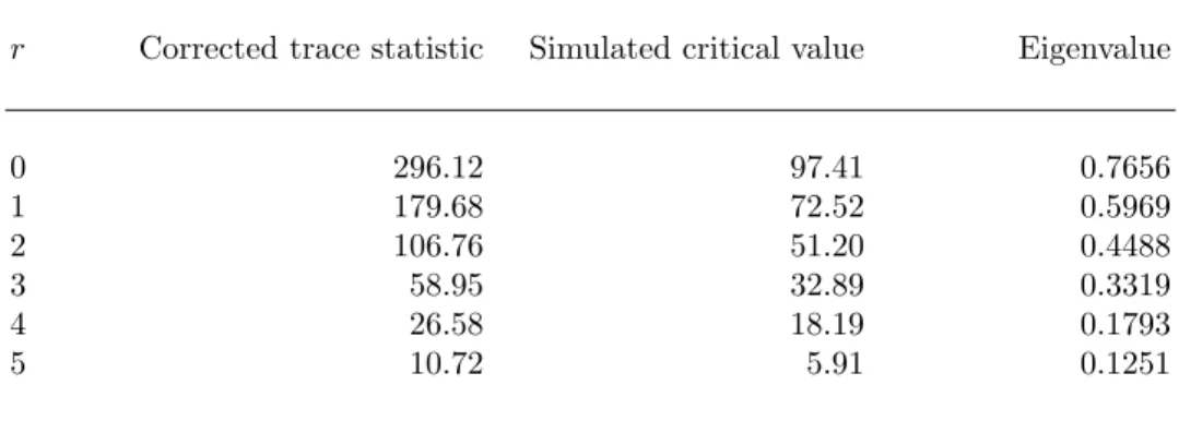
is estimated. Testing how many linearly independent stationary relations r there are

between the variables inXtis equivalent to test how many eigenvalues (λ) of αβ0 = Π are

significantly different from zero. For the tests I use the trace statistic, but as the sample size is relatively small, I apply its corrected version (Reimers, 1992)

LR(r) = −(T −np)

n X i=r+1

log(1−ˆλi). (5)

The particular null hypothesis is that the number of distinct cointegrating vectors is less

than or equal tor, the sequential testing procedure starts withH0: r= 0. Critical values

(7)

2 shows the corrected trace statistic and the simulated critical value for every possible r

as well as the eigenvalues of Π. The test results lead to conclude that Π has full rank,

so the vector process Xt is stationary. In the following, I therefore estimate equation (2)

including a linear time trend inZ.

4 Granger-causality results

The VAR can be estimated by OLS, using two lags of each endogenous variable in each equation. Because of some problems with serial correlation and heteroscedasticity in single equations, Newey-West standard errors were calculated which take account for serial correlation up to order 12. Granger-causality is investigated by testing whether

or not the coefficients of a variable’s lags jointly are equal to zero. P-values for the

corresponding F-statistics are reported in Table 3.

It is past information on policy rates that is found to be predictive for current bank lending rates. Nevertheless, there seems to be a transient reversal or correction in the interest rate transmission process as the first lag of the policy rate is negatively significant in the lending rate equation at the 5 % level. Dissemination of policy rate changes continues afterwards if the latter prove to be permanent. Given the information on past policy rate changes, the lags of the interbank rate do not provide an additional source for improving bank lending rate forecasts.

The fact that past inflation and credit growth changes are not strongly reflected in lending rates is indicative in favor of the housebank principle typical for Austria. Granger-causal for credit growth are the inflation rate as well as almost all interest rates (inflation leads the growth rate of commercial credit positively, the lending rate negatively).

Other interesting results, which are not directly related to the central question of interest rate transmission, emerge as well. For example, interest rates fail to Granger-cause the inflation rate. Policy-orientated interest rates could have been supposed to be a leading indicator for the inflation rate because of reverse causality (if expected inflation rises, interest rates move). Such an indicator effect is counteracted by interest rate changes actually lowering inflation. Also past credit growth cannot be used to obtain improved forecasts for the inflation rate and secondary market returns of private sector bonds cannot be predicted by lagged values of other interest rates and credit growth. Rising policy rates are forecasted by prior increases in credit growth and the interbank rate, but the policy rate is not led by past information on inflation.

5 Innovation accounting results

The next goal is to simulate the dynamic impact of unexpected exogenous “shocks” (or “innovations”) onto the variables in the system, especially onto the lending rate and credit

growth. If the VAR is stable, there exists an equivalent MA(∞) representation

Xt=τ+

∞

X i=0

θi²t−i. (6)

(8)

Because the components in et are not instantaneously uncorrelated, shocks could not be isolated from each other if they were represented by unexpected changes of the

reduced-form residuals. B0 is to be estimated and the θi matrices contain the so-called

impulse-response functions.

I identify the structural errors by restricting the contemporaneous relations between

the variables inB0via a Cholesky decomposition of Σ. With this,B0is forced to be a lower

triangular matrix. This means that the variable ordered first is not contemporaneously influenced by all the others in the system, only the first variable has an instantaneous effect on the second, and so on. The ordering of the variables therefore is crucial in this setting. Contemporaneous feedback relations cannot be accounted for with a Cholesky

decomposition, a recursive structure in form of a causal chain is imposed2_{. A different}

ordering would result in a different decomposition of Σ, different structural shocks and therefore different responses.

The causal chain I implemented is as follows: The inflation rate is assumed to be contemporaneously exogenous and ordered first, followed by the policy rate, the interbank rate, the bond yield and the lending rate. Credit growth is put last and therefore is restricted to not instantaneously influence any of the other variables. What I do not allow for is, for example, an impact of the interbank rate, the lending rate or credit growth on the policy interest rate within a month. I tried different plausible orderings to check the robustness of the impulse-response functions, but the applied one seems to be the most reasonable and acceptable “semi-structural” identification scheme. The structural errors are shocked by one unit in the following what amounts to 1-percentage-point shocks. Standard errors and 95 % confidence bands for all innovation accounting estimates are bootstrapped according to Runkle (1987) with 2000 replications.

The columns of Table 4 report contemporaneous (within-month) effects of a one-percentage-point shock in one variable on the others. Such a shock in the inflation rate, for example, leads to an increase in the lending rate of 0.08 percentage points within the same month. The instantaneous response of the bank lending rate to an unanticipated policy rate increase is 0.31 percentage points, whereas the comparable response to innovations in the interbank rate is smaller and not quite significant at the 5 % level. Lending rate responses will be more deeply investigated in the next two sections.

Some results from the impulse-response functions for a horizon of twelve months are the following: The bond yield (positively) responds to shocks in the policy and the interbank rate, but not to shocks in the inflation rate. Also the effects of shocks in the inflation rate onto the lending rate remain small over the year following the shock. There are no significant direct responses of credit growth due to shocks in the policy rate. But following an innovation in the interbank rate, credit growth significantly declines in

periodst andt+ 1. Responses of credit growth to structural shocks in the lending rate are

significantly negative and accumulate to approx. 6 percentage points over the 12-month horizon. The lending rate reacts to shocks in the bond yield in the medium run, but credit growth does not. So also the fact that bond issues cannot be taken seriously as a substitute for loans in Austrian corporate finance is represented in my results.

2_{A more appropriate identification rule can be defined by allowing free parameters above the diagonal} ofB0 with the appropriate number of restrictions maintained at the same time. All attempts to provide more economic structure (for example, to allow feedback between most of the interest rates) resulted in ill-mannered log-likelihood functions of the respective structural VAR, also with different starting values.

(9)

6 Lending rate responses

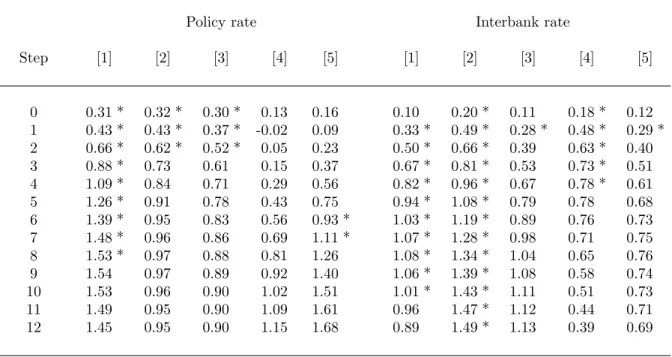
The response and the accumulated response of the lending rate following a 1-percentage-point innovation in the interbank rate can be found in Figure 2 together with 95 % confidence bands. The shock is fully disseminated and its transmission is completed after 6 months. A more detailed investigation of lending rate responses needs to address the following questions:

• Does the bank lending rate respond faster and more strongly to innovations in the

policy or the interbank rate?

• Is transmission faster if policy-determined rates increase than if they decrease?

• Descriptive statistics (see Table 1) and Figure 1 show that, on average, the difference

between the bank lending rate and the policy as well as the interbank rate fell sharply after 1998. But have patterns in interest rate transmission also changed since the European Monetary Union is in place?

To analyze these questions, I identify the following cases: The interest rate to be shocked (policy or interbank rate) increases, decreases or changes in one of these directions after

19983_{. The cases are represented by dummy variables and interaction terms. For example,}

for the case “the policy rate goes up” the VAR additionally contains a dummy variable (and two lags of it) that takes the value 1 if the policy rate has risen compared to the month before, as well as two lags of an interaction of this dummy with the policy rate. Only accumulated responses are discussed at this stage. The cases and the appendant results appear in different columns of Table 5, where columns [1] contain the estimates from the initial specification.

The different adjustment patterns indicate that, also in Austria, the lending rate sluggishly responds to changes in policy-controlled interest rates. An important finding is that there is a strong asymmetry in the transmission of policy rate innovations in the short term. After three months, 62 % of the shock are passed on to the bank lending rate in case of a rising policy rate, whereas after a decline the accumulated lending rate adjustment after three months is comparably low. From 1999 on, however, these differences in the short-term propagation of policy rate shocks declined. Responses of the bank lending rate to shocks in the interbank rate also prove to be asymmetric, but only in the longer term. In case of a falling interbank rate, transmission even stops about a half year after the shock (see the corresponding column [4] in Table 5). A long-term asymmetry also emerges for policy rate shock transmission. Decreases in the policy rate are more quickly passed on to bank lending rates after 1998. Accumulated responses for months 6 and 7 after the shock are significantly different from zero (see column [5] for shocks to the policy rate in Table 5).

3_{The fact that there are no data on commercial lending rates before 1995 complicates the interpretation} of the results because for the whole pre-EMU period applicable here the so-called “Lombard-Club” was in place. So if my results show that interest rate transmission in Austria became faster from 1999 on, this might also partly be due to the breakup of interest rate arrangements between large Austrian banks.

(10)

7 Conclusions

This study confirms and complements previous empirical findings on interest rate trans-mission with the result that there is considerable short-term stickiness of retail bank lend-ing rates also in Austria. The maximum instantaneous lendlend-ing rate adjustment is found in case of increases in the administered policy rate of which 32 % are passed through within one month. In this regard, there hardly is a difference to the European-level point estimate of De Bondt (2002).

Additionally, the interest rate transmission process in Austria is asymmetric as the adjustment paths of the lending rate differ markedly subject to the direction of changes in policy and money market rates. Not in every case the final adjustment of the interest rate on short-term commercial loans is complete.

Institutional changes, in particular the implementation of the European Monetary Union (EMU), had significant effects on the interest rate pass-through process. But a quicker transmission, as suggested by Mojon (2000) and De Bondt (2002), is not uniformly supported by the Austrian data. Lending rate adjustment especially is stronger (faster) following decreases in the policy rate after 1998, but is weaker (slower) in case of rising interbank and policy rates within the EMU-period.

All the results for lending rate responses suggest that a shift in the relative im-portance of interest rate innovations for retail bank lending rates seems to have taken place in the last years. The increasingly relevant determinant (or leading indicator) for commercial credit interest rates in recent times is the policy rate. This matches well with the observation that changes in key interest rates are more publicly recognized and de-bated since the European Central Bank is responsible for monetary policy. But also the economic climate at times of the interest rate decreases after September, 11, 2001 might partly be responsible for the stronger and faster transmission found to happen if policy rates go down after 1998.

Future research may deal with determinants of the transmission process that are not covered here explicitly or assumed to be constant. These factors comprise the state of the economy in an interest rate or business cycle, shifts in the demand for and the riskiness of loans as well as changes in the banks’ markups.

References

[1] BORIO, C.E.V. and W. FRITZ (1995), “The response of short-term bank lending rates to policy rates: A cross-country perspective”, Working Paper No. 27, Monetary and Economic Department, Bank for International Settlements, Basle.

[2] BRAUMANN, B. (2002), “Financial liberalization in Austria: Why so smooth?”, in: Oesterreichische Nationalbank,Financial Stability Report 4, Vienna, 100-114.

[3] COTTARELLI, C. and A. KOURELIS (1994), “Financial structure, bank lending rates, and the transmission mechanism of monetary policy”,IMF Staff Papers41, 587-623.

[4] De BONDT, G. (2002), “Retail bank interest rate pass-through: New evidence at the Euro area level”, Working Paper No. 136, European Central Bank, Frankfurt.

[5] DICKEY, D.A. and W.A. FULLER (1979), “Distributions of the estimators for autoregressive time series with a unit root”,Journal of the American Statistical Association74, 427-431.

(11)

[6] DONNAY, M. and H. DEGRYSE (2001), “Bank lending rate pass-through and differences in the transmission of a single EMU monetary policy”, Discussion Paper DPS 01.17, Center of Economic Studies, Katholieke Universiteit, Leuven.

[7] ELLIOTT, G., ROTHENBERG, T.J. and J.H. STOCK (1996), “Efficient tests for an autoregressive unit root”,Econometrica64, 813-836.

[8] FRANSES, P.H. and B. HOBIJN (1997), “Critical values for unit root tests in seasonal time series”,

Journal of Applied Statistics24, 25-47.

[9] HAMILTON, J.D. (1994),Time series analysis, Princeton University Press.

[10] JOHANSEN, S. (1995), Likelihood-based inference in cointegrated vector auto-regressive models, Oxford University Press.

[11] JOHANSEN, S. and B. NIELSEN (1993), “Asymptotics for cointegration rank tests in the presence of intervention dummies”, Manual for the simulation program DisCo, Institute of Mathematical Statistics, University of Copenhagen, http://www.math.ku.dk/˜sjo.

[12] KWIATOWSKI, D., PHILLIPS, P.C.B., SCHMIDT, P. and Y. SHIN (1992), “Testing the null hypothesis of stationarity against the alternative of a unit root: How sure are we that economic time series have a unit root?”,Journal of Econometrics54, 159-178.

[13] L ¨UTKEPOHL, H. (1999), “Vector autoregressions”, Discussion Paper No. 1999-4, Interdisciplinary Research Project 373, Humboldt University, Berlin.

[14] MARDIA, K.V. (1980), “Tests for univariate and multivariate normality”, in: KRISHNAIAH, P. R. (ed.),Handbook of Statistics 1, North-Holland, New York, 279-320.

[15] MOJON, B. (2000), “Financial structure and the interest rate channel of ECB monetary policy”, Working Paper No. 40, European Central Bank, Frankfurt.

[16] REIMERS, H.-E. (1992), “Comparison of tests for multivariate cointegration”,Statistical Papers33, 335-359.

[17] RUNKLE, D.E. (1987), “Vector autoregressions and reality”, Journal of Business and Economic Statistics5, 437-442.

[18] SANDER, H. and S. KLEIMEIER (2002), “Asymmetric adjustment of commercial bank interest rates in the Euro area: An empirical investigation into interest rate pass-through”, Kredit und Kapital35, 161-192.

[19] TOOLSEMA, L.A., STURM, J.-E. and J. De HAAN (2001), “Convergence of monetary transmission in EMU: New evidence”, Working Paper No. 465, CESifo, Munich.

[20] WETH, M.A. (2002), “The pass-through from market interest rates to bank lending rates in Ger-many”, Discussion Paper 11/02, Economic Research Center, Deutsche Bundesbank, Frankfurt.

(12)

A

Figures and Tables

Figure 1: Interest rates.

0 1 2 3 4 5 6 7 8 9 10 1996:01 1997:01 1998:01 1999:01 2000:01 2001:01 2002:01

Policy rate Interbank rate Lending rate

Figure 2: Lending rate responses to a 1-percentage-point shock in the interbank rate.

−.1 0 .1 .2 .3 0 1 2 3 4 5 6 7 8 9 10 11 12 Response 0 .5 1 1.5 2 0 1 2 3 4 5 6 7 8 9 10 11 12 Accumulated response

Notes: The figure reports responses and accumulated responses (in percentage points) for the 12 months following the shock. Dashed lines display the appendant 95 % confidence intervals. The graphs also include the within-month adjustment of the lending rate (period 0).

(13)

Table 1: Descriptive statistics.

Variable Mean Standard error Minimum Maximum

Full sample period: March 1995 - December 2002

Inflation rate 1.69 0.77 0.20 3.27 Policy rate 3.49 0.66 2.50 4.81 Interbank rate 3.72 0.62 2.58 5.09 Bond yield 5.34 0.79 3.53 7.19 Lending rate 6.58 0.79 5.41 8.72 Credit growth 0.39 1.00 -2.83 3.69 Lending rate - policy rate 3.09 0.70 1.92 4.36 Lending rate - interbank rate 2.86 0.66 1.79 4.26

Subperiod 1: March 1995 - December 1998

Subperiod 2: January 1999 - December 2002

(14)

Table 2: Cointegration rank test results.

r Corrected trace statistic Simulated critical value Eigenvalue

0 296.12 97.41 0.7656 1 179.68 72.52 0.5969 2 106.76 51.20 0.4488 3 58.95 32.89 0.3319 4 26.58 18.19 0.1793 5 10.72 5.91 0.1251

Notes: The testing procedure is sequential, starting withH0: r= 0. If the null hypothesis is

rejected, the next step is a test ofH0:r≤1, and so on.

Table 3: Granger-causality test results.

Inflation Policy Interbank Bond Lending Credit Equation of rate rate rate yield rate growth

Inflation rate 0.286 0.392 0.505 0.830 0.125 0.828 Policy rate 0.892 0.012 0.012 0.109 0.087 0.017 Interbank rate 0.455 0.558 0.000 0.018 0.348 0.915 Bond yield 0.809 0.626 0.930 0.000 0.781 0.305 Lending rate 0.232 0.002 0.168 0.000 0.000 0.759 Credit growth 0.004 0.000 0.000 0.195 0.000 0.009 Notes: Granger-causality is examined by testing whether the coefficients of both lags of a variable jointly are zero in a particular equation. The table reportsp-values for the accordingF-statistic. The rows of the table illustrate the test results equation by equation, the columns show the test results for the variable in the header.

(15)

Table 4: Within-month responses.

Within-month Inflation Policy Interbank Bond Lending response of rate rate rate yield rate

Inflation rate Policy rate 0.03 Interbank rate 0.02 0.78 * Bond yield 0.04 0.83 * 0.43 * Lending rate 0.08 * 0.31 * 0.10 -0.04 Credit growth 0.59 * -0.16 -1.08 * 0.58 * -0.91 Notes: Each row of the table reports by how much a variable responds to 1-percentage-point shocks in the column-heading series within one month. There is no table entry for responses to own shocks and if the response is restricted to be zero in the identification scheme of the structural shocks. Responses marked with an asterisk are significantly different from zero at the 5 % level.

Table 5: Accumulated responses of the bank lending rate.

Policy rate Interbank rate

Step [1] [2] [3] [4] [5] [1] [2] [3] [4] [5] 0 0.31 * 0.32 * 0.30 * 0.13 0.16 0.10 0.20 * 0.11 0.18 * 0.12 1 0.43 * 0.43 * 0.37 * -0.02 0.09 0.33 * 0.49 * 0.28 * 0.48 * 0.29 * 2 0.66 * 0.62 * 0.52 * 0.05 0.23 0.50 * 0.66 * 0.39 0.63 * 0.40 3 0.88 * 0.73 0.61 0.15 0.37 0.67 * 0.81 * 0.53 0.73 * 0.51 4 1.09 * 0.84 0.71 0.29 0.56 0.82 * 0.96 * 0.67 0.78 * 0.61 5 1.26 * 0.91 0.78 0.43 0.75 0.94 * 1.08 * 0.79 0.78 0.68 6 1.39 * 0.95 0.83 0.56 0.93 * 1.03 * 1.19 * 0.89 0.76 0.73 7 1.48 * 0.96 0.86 0.69 1.11 * 1.07 * 1.28 * 0.98 0.71 0.75 8 1.53 * 0.97 0.88 0.81 1.26 1.08 * 1.34 * 1.04 0.65 0.76 9 1.54 0.97 0.89 0.92 1.40 1.06 * 1.39 * 1.08 0.58 0.74 10 1.53 0.96 0.90 1.02 1.51 1.01 * 1.43 * 1.11 0.51 0.73 11 1.49 0.95 0.90 1.09 1.61 0.96 1.47 * 1.12 0.44 0.71 12 1.45 0.95 0.90 1.15 1.68 0.89 1.49 * 1.13 0.39 0.69 Notes: The table reports accumulated responses of the lending rate to a 1-percentage-point shock in either the policy or the interbank rate for various subsequent months (steps). The table entries for step 0 refer to responses within the month the shock occured. Responses marked with an asterisk are significantly different from zero at the 5 % level.

For both policy and interbank rate shocks there are five cases. Column [1] tabulates the initial estimates. For the scenarios tabulated in columns [2] to [5], the VAR includes lagged interaction terms and contemporaneous as well as lagged shift dummies for the following events concerning the respective shocked interest rate in time periodt: [2] Increase, [3] Increase after 1998, [4] Decrease, [5] Decrease after 1998.

(16)

B

Description of the data

Denotation Description and source

Inflation rate Inflation rate in %, growth rate of a chained consumer price index (CPI, base year 2000) relative to the value of this CPI a year before. Source of the CPI: Statistik Austria.

Policy rate March 1995 - December 1995: Short-term open-market operations interest rate. Source: Austrian Central Bank (Oesterreichische Nationalbank, OeNB). January 1996 - December 1998: Interest rate on open-market tenders. Source: OeNB. January 1999 - December 2002: Main refinancing operations rate (fixed rate up to the end of June 2000, average rate of variable rate tenders after June 2000). Source: European Central Bank (ECB).

Interbank rate March 1995 - December 1998: 3 month Vienna interbank offered rate. Source: OeNB. January 1999 - December 2002: 3 month Euro interbank offered rate (Eu-ribor). Source: ECB.

Bond yield Secondary market return on listed bonds issued by Austrian non-banking institu-tions (excluding bonds issued by the public sector) with a fixed interest rate and more than one year remaining to maturity. Source: OeNB.

Lending rate Short-term commercial credit rate (average interest rate on new short-term loans to enterprises reported by a sample of 41 Monetary Financial Institutions). Source: OeNB.

Credit growth Growth rate of commercial credit (outstanding accounts of domestic non-bank and non-financial enterprises). Source: OeNB.

The sample starts in March 1995 and ends in December 2002. Interest rates and commercial credit are in nominal terms.

Dummy variables represent the following events: The definition of the commercial credit series was altered at the end of 1995; European level interest rates replace some of the national rates from January 1999 on; the basket of goods and services of the Austrian CPI changed in January 1996 and 2000; in July 2000 the ECB shifted from fixed rate to variable rate tenders in refinancing operations.