Image Denoising Using A Generative Adversarial Network

Image Denoising Using a Generative Adversarial Network

Abeer Alsaiari

_{, Ridhi Rustagi}

Dept. of Computer Science University of Illinois at Chicago

Chicago, USA

e-mail: 1_{[email protected],} 2_{[email protected]}

A’aeshah Alhakamy

Indiana University–Purdue University Indianapolis, USA e-mail: 3_{[email protected]}

Manu Mathew Thomas

_{, Angus G. Forbes}

University of California, Santa Cruz Santa Cruz, USA

e-mail: 4_{[email protected],} 5_{[email protected]}

Figure 1. Gaussian noise image (left), our denoised image (middle) and ground truth photorealistic image (right).

Abstract—Animation studios render 3D scenes using a technique called path tracing which enables them to create high quality photorealistic frames. Path tracing involves shooting 1000’s of rays into a pixel randomly (Monte Carlo) which will then hit the objects in the scene and, based on the reflective property of the object, these rays reflect or refract or get absorbed. The colors returned by these rays are averaged to determine the color of the pixel. This process is repeated for all the pixels. Due to the computational complexity it might take 8-16 hours to render a single frame. We implemented a neural network-based solution to reduce the time it takes to render a frame to less than a second using a generative adversarial network (GAN), once the network is trained. The main idea behind this proposed method is to render the image using a much smaller number of samples per pixel than is normal for path tracing (e.g., 1, 4, or 8 samples instead of, say, 32,000 samples) and then pass the noisy, incompletely rendered image to our network, which is capable of generating a high-quality photorealistic image.

Keywords-image denoising; rendering; deep learning

I. INTRODUCTION

Computer-generated imagery is a core component of movies, video games, and commercials. From the early stage, efforts are made to enhance the production of 3-dimensional images and many algorithms are proposed to efficiently render 3D scenes. During the 1960’s and early 1970’s, algorithms are proposed to render 3D scenes with enhanced realism. For example, algorithms like hidden-surface and hidden-line are proposed to resolve the visibility problem. Many other algorithms have been proposed over the years for photorealistic rendering [1]. Nowadays, animation movie studios, such as Pixar and Dreamworks, render their 3D scenes using a technique called path tracing, which generates high-quality photorealistic frames. Path tracing involves shooting 1000’s of rays into a pixel randomly (Monte Carlo), which will then hit the objects in the scene and, depending upon the reflective property of the object, will reflect or refract or become absorbed. The colors generated by these rays are averaged to obtain the color of the pixel, and this process is repeated for all pixels. Rendering scenes frame by frame is computationally expensive and time consuming, as thousands of rays per pixel are needed in order to render a photorealistic image. GPU technology and efficient software APIs have increased

____________________________________________________

This is the author's manuscript of the article published in final edited form as:

Alsaiari, A., Rustagi, R., Alhakamy, A., Thomas, M. M., & Forbes, A. G. (2019). Image Denoising Using A Generative Adversarial Network. 2019 IEEE 2nd International Conference on Information and Computer Technologies (ICICT), 126–132. https://doi.org/10.1109/INFOCT.2019.8710893

rendering speeds, but path tracing is still nowhere close to real-time rendering. Due to the computational complexity it can take hours to render even a single frame.

Motivated by this problem, several attempts are being made to speed up the process of obtaining high quality images. Using a few samples to render a 3D scene can be quickly evaluated, but the inaccuracy of this estimate appears as noise in the final image. This problem can be addressed using a denoising mechanism to generate a high-quality noise-free image. Image denoising methods are applicable to any noisy images either CGI, scanned images or images taken by a camera. Limitations in signal transmission equipment like cameras and scanners are the main source of noise in images. Enhancing the quality of images is important in many applications including, but not limited to, medical images and geographical pictures. In addition, a decent visual level is important for a better user experience in all applications.

The most recent promising results for many problems in image processing, including image denoising, are accomplished in particular by convolutional neural networks (CNNs). Deep learning networks generate astounding results in solving different tasks across a wide range of domains, often outperforming traditional methods. CNNs have a similar architecture as conventional deep learning neural networks, but they explicitly assume the input is an image. They have been used as an underlying architecture for image processing such as in image classification, image denoising, and super resolution. Dong et al. [2] claims that an image-denoising pipeline that uses example-based Super Resolution methods, such as the sparse-coding-based method, could be equivalent to the convolutional neural network procedure. However, sophisticated results depend on the power of the network design and training process. With respect to visual recognition tasks, the depth of the network is of central importance. The deeper the network, the better the result. Although training deep networks is very hard because of the emergence of the vanishing gradient problem, some network designs have been proposed to address this issue. Residual nets [3] are powerful networks that can handle very deep depths by heavy use of skip connections and batch normalization.

In this work, we propose a neural network-based solution for reducing 8-16 hours to a couple of seconds using a Generative Adversarial Network. The main idea behind this proposed method is to render using a small number of samples per pixel, which creates a noisy output image, and then pass the noisy image to our network, which generates a photorealistic image, in effect denoising the image. Our proposed network is based on ResNet [3]. The key for our work is the defined loss function and the very deep GAN. We define a refined perceptual loss that preserves not only color and texture, but also properties of the scene like motion blur and depth of field.

The rest of the paper is organized as follows. We provide an overview of the most related work in section 2. Section 3 shows the architecture of our proposed GAN. In Section 4, we discuss our experiments and achieved results. Finally, we conclude in Section 5.

II. RELATED WORK

Artificial neural networks have been widely used for regression problems that map continuous vectors of input to another continuous vector of output by minimizing an optimization function. In [4], a multi-layer perceptron neural network is learned for image denoising formulated as a regression problem. Pairs of noisy and clean patches are used to estimate the network parameters that minimize the difference between the noisy and clean patches. Each layer applies weights to patches, which are then sent to the next layer before outputting a new image. This output is compared to ground truth value. To update the network parameters, backpropagation is used and the mean squared error is minimized. The learned MLP network is used then to denoise images by dividing the image into overlapping patches as continuous input vectors. Each patch is denoised and the average of overlapping patches is calculated to produce the denoised image.

MLP is also used in [5] to filter out Monte Carlo noise from images. Monte Carlo rendering can produce high quality images but requires calculating many expensive rays resulting in lengthy render times. A few samples can be quickly evaluated but will produce a noisy image. They addressed this problem by applying a denoising filter to produce a pleasing high-quality image. To achieve that, they observed that the noisy image and the ideal filter parameters have a complex underlying correlation. The rendered image is a set of primary features at each pixel like screen position, color, shading, etc. A set of statistical secondary features of each pixel in relation to other pixels is achieved by processing the pixel local neighborhood. Then, an MLP network is learned with these features to output a set of filter parameters. The filter module applies the learned parameters to the noisy rendered image to filter the pixels and generate the filtered image.

Convolutional networks have been used as architecture for the image denoising process. Jain and Seung [6] proposed an unsupervised learning approach for image denoising using the convolutional network. In contrast to the typical structure of a convolutional network that outputs a single score, their network restores a denoised image from an input that is subjected to the Gaussian noise model. The network outperformed previous approaches with 4 hidden layers and 24 feature maps per hidden layer. During the unsupervised learning, the network is trained with the Berkeley segmentation dataset. This dataset contains noise free images and therefore they formulated the denoising problem as an unsupervised learning process. During the training, a noise function with different variations is integrated into the training process to synthesize noisy training samples from noise free images. The network is then trained to denoise images by minimizing the reconstruction error of noisy samples as a loss function. That is, it’s trained to minimize the difference between the free noise image and the noisy reconstructed image.

Another related problem that is solved using convolutional networks is the single image super resolution. Super resolution processes a low-resolution image to

estimate its high-resolution counterpart. The convolution network is proposed in [2] for single image super resolution. Similar to [6], the input image is divided into overlapping patches. Using two convolution operations, conceptually high-resolved patches are computed and then aggregated to compose a high-resolution output image. Due to the difference in resolutions, the input image is upscaled first to the desired resolution as a preprocessing step. The parameters of the mapping function are learned during the training by minimizing the mean squared error between the reconstructed image and the ground truth image.

SRGAN [7] introduces an approach similar to ours. Unlike previously proposed convolutional networks for image super resolution that are based on the mean squared error as an optimization function, they propose a new loss function that resolves perceptually satisfying high-resolution image. The architecture consists of a very deep residual net architecture, which is a GAN-based network consisting of

discriminator and generator networks. The generator network is trained to generate an indistinguishable image from the ground truth, fooling the discriminator with the reconstructed image. Similarly, the discriminator is trained to distinguish reconstructed images from real images. The training of the network is achieved by minimizing the perceptual loss function, that is, by minimizing the weighted sum of its components: content loss and adversarial loss. Instead of relying on pixel-wise error measures such as MSE-based optimization, they proposed a novel perceptual loss function consisting of content loss and adversarial loss. The goal of adding content loss is to handle the solution with respect to perceptual high-level features. The content loss is based on perceptual similarity. Using pre-trained 19-layers VGG network, feature maps are obtained for the reconstructed and reference images. The feature map is computed by encoding each image vector by layer filters.

The difference between features maps of reconstructed images and reference images is computed as a Euclidean distance to define the content loss. The adversarial loss makes the discriminator and generator push the solution to the natural image space in which the generator tries to fool the discriminator with the reconstructed image and the discriminator tries to distinguish the reconstructed image from the real image. The architecture is based on the ResNet [3] deep convolutional network. ResNet is defined to enhance the training of very deep networks by adding “shortcut” connections that feed the input to deep layers. The residual layers then retain spatial information and tune the output with reference to the input.

Recent work by Chaitanya et al. [11] and Bako et al. [12] also explores the application of deep learning to denoising images, but our approach differs in that it utilizes a GAN architecture.

III. METHOD

We built a GAN network structure for image denoising, which, like SRGAN, is based on ResNet [3]. A generator network is trained to generate noise free images through competing with a discriminator network, using ground truth reference images to improve the quality of the generated

images. Our architecture makes use of residual blocks, skip connections, and batch normalization. In our initial implementation, due to training time limitations, we used three residual blocks. Having a larger number of residual blocks would increase the training accuracy significantly, but at with the incurred expense of requiring longer training times.

A. Generator Network

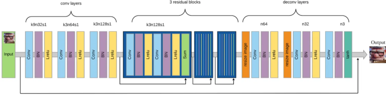
The goal of single image denoising is to generate a photorealistic image with high quality. The generator should be able to fill in the noises with neighboring pixel colors without losing any information present in the original image. We adopt a symmetric structure, similar to traditional CNN frameworks, that directly learns an end-to-end mapping from input noisy images to their corresponding ground truth. A set of three convolutional layers, using batch normalization and Lrelu activation, are stacked in the front of the network, which extract semantic attributes from the input image.

Three residual blocks each containing two convolutional layers are used to increase the depth of the network. We involve symmetric skip connections in this sub-network to improve efficiency in training and to promote faster convergence. The skip connections feed the input to the deep layers so each residual layer tune the output with reference to input and retain spatial information. These are followed by three sub-pixel convolutional layers, each corresponding to the convolutional layers in the front of the network. Each sub-pixel convolutional layer consists of a resized image block followed by convolutional layer. The images are resized from 64x64 to 128x128, and the final image output is of size 256x256. We use sub-pixel convolutional layers instead of deconvolutional layers to avoid checkboard like patterns in the image. Since the sub-pixel convolution is similar to deconvolution, we will refer to those layers as

deconvolutional layers in this paper. The first two deconvolutional layers have Lrelu activations and the final deconvolutional layer providing the denoised output has a sigmoid activation. For all layers we use stride of 1. The generator network is as follows:

where CBL(K) is a set of K-channel convolutional layers followed by batch normalization and Lrelu activation, and DBL(K) is a set of K-channel deconvolutional layers followed by batch normalization and Relu activation. Skip connections are added via every two layers.

B. Discrimintator Network

The goal of denoising a noisy image is not only to make the denoised result visually appealing and quantitatively comparable to the ground truth, but also to be of photorealistic high quality. Therefore, we included a learned discriminator sub-network to classify if each input image is real or fake. We use five convolutional networks with Batch Normalization and Lrelu activation throughout discriminator network.

CBL(K) – CBL(K*2) – CBL(K*2*2) – CBL(K*2*2) – CBL(K*2*2) – CBL(K*2*2) – DBL(K*2) – DBL(K) –

Figure 2. Generator network.

Figure 3. Discriminator network. Once we calculate the learned feature from a set of these

Conv-BN-Lrelu, a sigmoid function is stacked at the end to map the output to a probability score normalized to [0,1]. The structure of the discriminator sub-network is as follows:

where CB(K2) is a set of K2 channel convolutional layers followed by batch normalization and C(1) is a set of 1- channel convolutional layers.

C. Refined Loss Function

To ensure that the results have good visual and quantitative scores along with good discriminatory performance, we combine pixel-to-pixel Euclidean loss (pixel loss), feature loss, smooth loss and adversarial loss together with appropriate weights.

Adversarial loss helps the generator to produce better output to fool the discriminator. Pixel loss helps to correctly fill the noise with colors by comparing every pixel of generated image with the ground truth image (Euclidean distance). Feature loss helps to extract features accurately and is calculated in the same way that pixel loss is, but is determined by examining the image data extracted from the Conv2 layer of VGG16 network. We add a smooth loss function to the existing loss functions. The intuition behind this is to prevent “checkboard” artifacts across neighboring pixels in the image. To determine the smooth loss, we slide a copy of the generated image one unit to the left and one unit down and then calculate the Euclidean distance between the

shifted images. The new loss function is then defined as follows:

(3)

where LA represents adversarial loss (loss from the discriminator D), LP is pixel loss (pixel-to-pixel Euclidian distance between generated image and ground truth image), Lf is feature loss (pixel-to-pixel Euclidian distance between generated image and the ground truth image from the Conv2 layer of VGG16), and Ls is smooth loss. λa, λp, λf and λs are pre-defined weights for adversarial loss, pixel loss, feature loss and smooth loss, respectively.

IV. EXPERIMENT AND RESULTS

In this section, we present details of our experiments investigating our denoising network and discuss the dataset and training details.

A. Dataset and Training

Due to the lack of availability of large size datasets for training and evaluation of single image denoising, we synthesized a new set of training and testing samples in our experiments. We downloaded 40 Pixar movie image frames and added Gaussian noise to create the dataset, which included different standard deviations to generate a diverse training and test set— each image was denoised with five different amounts on noise. The training set consists of a total of 1000 images and the test set has 40 images. The images with noise form the set of observed images and the corresponding original images form the set of ground truth

images. All the training and test samples are resized to 256×144.

B. Model Details and Parameters

The entire network is trained on AWS p2.xlarge GPU using the TensorFlow framework. We used a batch size of 7 and the performed 10,000 training iterations. During training, we set λa=0.5, λp=1.0, λf=1.0 and λs=0.0001. We set K=32 and K2=48 for the generator and discriminator networks.

The first convolutional and deconvolutional layer of the Generator (G) is composed of kernel of size 9 with stride 1. All the other convolutional and deconvolutional layers in the Generator are composed of kernel of size 3x3, also with stride 1. All convolutional and deconvolutional layers in the first three layers of the discriminator (D) are composed of kernels of size 4×4 with a stride 2 and zero-padding by 1. The last two layers in D are composed of kernels of size 4x4 with a stride 1 and a zero-padding of 1.

Input Output Groundtruth Figure 4. Here we show resulting denoised output images using our approach using a test set of images

Input Output Input Output

Figure 5. Here we show resulting denoised output images using our approach, here using a test set of noisy photographs under natural light (which our network was not trained on).

Input Output

V. CONCLUSION

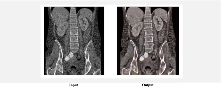
In conclusion, we developed a technique to perform image denoising using a generative adversarial network. Our network inputs a noisy image and generates a denoised version in less than a second, preserving edges and avoiding blurriness. Fig. 4 shows examples of output images in comparison to the ground truth. In our initial implementation, we trained our network with Gaussian noise, but we believe our generative adversarial network can be extended to handle both uniform and non-uniform noise, given an appropriate training dataset. Interestingly, we found that our network, trained with only 40 images from a specific domain for only 10,000 iterations, was successful at generating denoising images outside the domain it was trained. The network gave impressive results for grainy photos (Fig. 5), CT scans (Fig. 6), as well as frames from a noisy video capture.

In the future, we plan to include noise produced by Monte Carlo rendering. This is will allow us to investigate whether our technique can be used for making an efficient real-time path tracer which can be used for games or medical visualization applications. Currently, we generate the denoising image based on the available pixel color information. However, we would like to investigate whether or not our network can be modified to fill in noisy areas based on the semantics of the neighboring pixels, or by providing the network with additional information, such as a depth map of a 3d scene. Finally, we would also like to investigate whether our network can perform denoising with motion blur, depth of field, shadows, caustics, and global illumination [10].

The work described in this paper was initially developed as a class project for a graduate seminar in applied deep learning in the Electronic Visualization Laboratory at the University of Illinois at Chicago in early 2017. All code and instructions for running the code are available on GitHub at: http://github.com/CreativeCodingLab/ImageDenoisingGAN.

REFERENCES

[1] "3D Rendering History: Part 1. Humble Beginnings". The CGSociety. 2017.

[2] Dong, C., Loy, C.C., He, K. and Tang, X., 2016. Image super-resolution using deep convolutional networks. IEEE transactions on pattern analysis and machine intelligence, 38(2), pp.295-307. [3] He, K., Zhang, X., Ren, S. and Sun, J., 2016. Deep residual learning

for image recognition. In Proceedings of the IEEE Conference on Computer Vision and Pattern Recognition (pp. 770-778).

[4] Burger, H.C., Schuler, C.J. and Harmeling, S., 2012, June. Image denoising: Can plain neural networks compete with BM3D?. In Proceedings of the IEEE Conference on Computer Vision and Pattern Recognition (CVPR), 2012. (pp. 2392-2399).

[5] Kalantari, N.K., Bako, S. and Sen, P., 2015. A machine learning approach for filtering Monte Carlo noise. ACM Trans. Graph., 34(4):122.

[6] Jain, V. and Seung, S., 2009. Natural image denoising with convolutional networks. In Advances in Neural Information Processing Systems (pp. 769-776).

[7] Ledig, C., Theis, L., Huszár, F., Caballero, J., Cunningham, A., Acosta, A., Aitken, A., Tejani, A., Totz, J., Wang, Z. and Shi, W., 2016. Photo-realistic single image super-resolution using a generative adversarial network. arXiv preprint arXiv:1609.04802.

[8] Zhang, H., Sindagi, V. and Patel, V.M., 2017. Image De-raining Using a Conditional Generative Adversarial Network. arXiv preprint arXiv:1701.05957.

[9] Yeh, R., Chen, C., Lim, T.Y., Hasegawa-Johnson, M. and Do, M.N., 2016. Semantic Image Inpainting with Perceptual and Contextual Losses. arXiv preprint arXiv:1607.07539.

[10] Thomas, M.M. and Forbes, A.G., 2017. Deep Illumination: Approximating Dynamic Global Illumination with Generative Adversarial Networks. arXiv preprint arXiv:1710.09834.

[11] Chaitanya C.R., Kaplanyan A.S., Schied C., Salvi M., Lefohn A., Nowrouzezahrai D., and Aila T., 2017. Interactive Reconstruction of Monte Carlo Image Sequences Using a Recurrent Denoising Autoencoder. ACM Trans. Graph., 36(4):98.

[12] Bako S., Vogels T., McWilliams B., Meyer M., Novák J., Harvill A., Sen P., Derose T., Rousselle F., 2017. Kernel-predicting convolutional networks for denoising Monte Carlo renderings. ACM Trans. Graph., 36(4):97.