Running Krill Herd Algorithm on Hadoop: A Performance Study

Running Krill Herd Algorithm on Hadoop: A

Performance Study

Simone A. Ludwig

Fargo, ND, USA [email protected]

Abstract—The krill herd algorithm was introduced mimicking the herding behavior of krill individuals. The krill herd algorithm obtains the optimum solution by considering two factors, namely the density-dependent attraction of the krill, and the areas of high food concentration. The iterative optimization procedure is based on the time-dependent position of the krill individuals of (1) movement induced by other krill individuals, (2) foraging activity, and (3) random diffusion. In this paper, the krill herd algorithm is investigated when run on a Hadoop cluster. The algorithm was parallelized using MapReduce. Four different sets of experiments are conducted to evaluate the krill herd algorithm in terms of speed and accuracy. The first set of experiments investigates the execution time and speedup of the krill herd algorithm applied to six different benchmark functions. The second set of experiments investigates the varying dimensions of the Alpine benchmark function with regards to the effect on the execution time. The third set of experiments analyzes the effect of different krill sizes and numbers of maximum iterations on the execution time but also on the objective value. The fourth set of experiments compares the speed gain obtained when running the MapReduce-enabled version of the krill herd algorithm compared to the normal non-parallelized krill herd algorithm.

I. INTRODUCTION

Parallelization is the process where the computation is broken up into parallel tasks. The work done by each task, often called its grain size, can be as small as a single iteration in a parallel loop or as large as an entire procedure. When an application is broken up into large parallel tasks, the application is called a coarse grain parallel application. Two common ways to partition computation are task partitioning, in which each task executes a certain function, and data partitioning, in which all tasks execute the same function but on different data.

There are several different parallelization techniques avail-able, the oldest and most mature being message passing. The message passing methodology (MPI) [1] has been used as the

defacto standard for parallelization for years. However, the MapReduce programming model [2] has been introduced as an alternative model for data parallel programming. MapReduce presents a programming model that manages the distribution of the tasks automatically, and at the same time provides fault-tolerance and load balancing. The basic idea behind the MapReduce methodology is that the problem is formulated as a functional abstraction using two main operations: the

mapoperation and reduceoperation.

Apache Hadoop [3] is the commonly used MapReduce implementation, and it is an open source software framework

that supports data-intensive distributed applications. It en-ables applications to work with thousands of computationally independent computers and petabytes of data. The Hadoop Distributed File System (HDFS - storage component) and MapReduce (processing component) are the main core com-ponents of Hadoop. HDFS enables high-throughput access to the data while maintaining fault tolerance by creating multiple replicas of the target data blocks. MapReduce is designed to work together with HDFS to provide the ability to move computation to the data and not vice versa. Figure 1 shows the Hadoop architecture diagram with interactions between its components. The Hadoop architecture consists of the HDFS, which is responsible for the reading and writing of data as well as the storage in the data nodes. The job driver is responsible to interact with the job tracker whose task it is to manage the

map andreduce tasks via the task trackers [5]. The input of the computation is a set of key-value pairs, and the output is a set of output key-value pairs. An algorithm to be parallelized needs to be expressed asmapandreducefunctions. Themap

function takes an input pair and returns a set of intermediate key-value pairs. The framework then groups all intermediate values associated with the same intermediate key and passes them to the reduce function. The reduce function uses the intermediate key and set of values for that key. These values are merged together to form a smaller set of values. The intermediate values are forwarded to the reduce function via an iterator. More formally, themapandreducefunctions have the following types:

map(k1, v1)→list(k2, v2)

reduce(k2, list(v2))→list(v3)

MapReduce technologies have also been adopted by a growing number of groups in industry (e.g., Facebook [6], and Yahoo [7]). In academia, researchers are exploring the use of these paradigms for scientific computing, such as in areas of Bioinformatics ([8], [9]) and Geosciences [10], where codes are written using open source MapReduce tools. In the past, these users have had a hard time running their Hadoop codes on traditional High Performance Computing (HPC) systems that they had access to. This is because it has proven difficult for Hadoop to co-exist with existing HPC resource management systems, since Hadoop provides its own scheduling, and manages its own job and task submissions as well as tracking.

Fig. 1. Hadoop Architecture Diagram [4]

over the resources that they manage, it is a challenge to enable Hadoop to co-exist with traditional batch systems such that users may run Hadoop jobs on these resources. Furthermore, Hadoop uses a shared-nothing architecture [11], whereas traditional HPC resources typically use a shared-disk architecture, with the help of high performance parallel file systems.

In this paper, a krill herd algorithm is parallelized and evaluated when run on a Hadoop cluster. The organization of this paper is as follows: In Section II, related work in the area of MapReduce and Hadoop in terms of nature-inspired algorithms is presented. Section III introduces and describes the krill herd algorithm including the algorithmic description and the equations involved. In Section IV, the experiments conducted are given and the results obtained are outlined. Section VI describes the conclusions reached from this study.

II. RELATEDWORK

A review of nature-inspired algorithms parallelized with the MapReduce framework is summarized. For example, a Genetic Algorithm (GA) was first implemented with the MapReduce framework in [12] featuring a hierarchical reduction phase. Another MapReduce-enabled GA was introduced in [13], where the authors investigated the convergence as well as the scalability of their algorithm applied to the BitCounting prob-lem. An application of GA using MapReduce was proposed in [14]. The authors implemented a GA algorithm for job shop scheduling problems running experiments with various

population sizes and on clusters of various sizes.

McNabb et al. evaluated the PSO MapReduce model on a radial basis function as the benchmark [15]. The authors state that their approach scaled well for optimizing data-intensive functions. An overlay network optimization algorithm based on PSO was parallelized using MapReduce [16]. Wu et al. proposed a MapReduce-based ant colony approach [17], and outlined the modeling with the MapReduce framework. The fireworks algorithm has been parallelized using the MapRe-duce methodology applied to benchmark functions achieving good speedup [18].

Furthermore, the parallelization of nature-inspired algo-rithms using the MapReduce framework applied to data mining has been done. For example in the clustering area, two MapReduce-enabled algorithms were implemented, one using PSO [4], and the other using a Glowworm Swarm Optimization (GSO) approach [19]. Furthermore, a fuzzy c-means clustering algorithm has been parallelized in [20].

III. KRILLHERDALGORITHM

The krill herd algorithm is a nature-inspired algorithm mimicking the behavior of krill individuals in krill herds. The algorithm was proposed by Gandomi and Alavi in 2012 [21]. The krill herd algorithm describes observations made on the Antarctic Krill species [22], which is considered as one of the best studied marine animal species. These krills are capable of forming large groups of swarms with no parallel orientation existing between them. For decades, studies have

been carried out to understand the herding mechanism of the krills, and the individual distribution of the krills among the herds. The studies identified some of the factors in spite of some uncertainties observed, mainly, the basic unit of the organization is the krill swarm. Another important factor considered is the presence of a predator. When one krill is affected by a predator, that krill is abandoned from the herd, which in turn reduces the density of the swarm. The increase in the krill density, and the distance from the food is always observable during the formation of the herds.

The krill herd algorithm was devised such that the optimum solution is obtained by considering the two main objectives of the density-dependent attraction of the krill, and the areas of high food concentration. The relation between the objective function and the krill position is proportionate. The global optimum implies the minimum distance of a krill from the highest density and food. The krill individuals always try to move towards the best solution during this process, and thus, improve the objective function.

The main process in the algorithm are the following motion updates:

• Induced movement (N)

• Foraging (F)

• Random diffusion (D)

The induced movement relates to the density maintenance of the krill herd given each krill individual and is given by:

Ni(t+ 1) =Nmaxαi+ωnNi(t) (1)

whereαi=αlocali +α target

i ,Nmax is the maximum induced

speed, ωn is the inertia weight,αlocali is the local effect the ith krill individual has on its neighbors, αtarget_i is the best solution of the ith krill individual and is determined by:

αtarget_i =CbestKi,bestXi,best (2)

where Cbest defines the effect of αtarget_i on the ith krill individual. Cbest is determined by:

Cbest= 2(r+I

Imax

) (3)

whereris a random number in [0,1],iis the current iteration, andImax is the maximum number of iterations. The foraging

update is done by:

Fi(t+ 1) =Vfβi+ωfFi(t) (4)

where βi =βif ood+B best

i , Vf is the foraging speed, ωf is

the inertia weight, andBbest_i indicates the food attraction and is the best solution of theithkrill individual so far. The third motion update is mimicking the physical diffusion by random activity and is given as:

Di(t+ 1) =Dmax(

1−I Imax

)δ (5)

whereDmax _{represents the maximum diffusion speed, and δ}

is a random directional vector in [-1,1]. The position of each krill individual is updated as follows:

Xi(t+ 1) =Xi(t) + ∆xi(t) (6)

∆xi(t) =Ni(t) +Fi(t) +Di(t) (7)

Once the position update is complete, the evolutionary opera-tors such as crossover and mutation are applied as in [21].

The algorithmic description is given by Algorithm 1. The algorithm starts with the random initialization of the krill population reading in the necessary variables such as the forag-ing speed, maximum diffusion speed, and maximum induced speed. Then, the krill population is evaluated by determining the objective value of all krill individuals. Afterwards, the main loop of the algorithms starts by first sorting the krill population from the best to the worst individual. Next follows the four step process that is done on each krill individual and repeated until the stopping criterion has been reached: (1) motion updates (induced movement, foraging, random diffusion) are calculated (Eq. 1-6); (2) genetic operators are applied; (3) krill individual’s position is updated (Eq. 7); and (4) evaluation of objective function of krill individual. At the end of the algorithm, the best krill (solution) is returned. The stopping criterion used is the completion of a predefined number of function evaluations.

Algorithm 1 krill herd algorithm

Random initialization of krill population Initialization of foraging speed

Initialization of maximum diffusion speed and induced speed Evaluate all krill individuals

whilestopping criterion is not metdo

Sort the krill population from best to worst

forall krillsdo

Calculate motion updates (Eq. 1, 5, 6) Apply genetic operators

Update the krill individual’s position (Eq. 7) Evaluate the krill individual

end for end while

return best krill

IV. EXPERIMENTALSETUP

This section describes the MapReduce enabled krill herd algorithm implementation, followed by the parameters used for the experiments, the benchmark functions to be optimized, and the execution environment used for running the experiments.

A. MapReduce-enabled Krill Herd Algorithm

Algorithm 2 describes the implementation of the MapRe-duce enabled krill herd algorithm. The main krill herd al-gorithm code is run in the Map function, and the Reduce function aggregates the fitness values that were received by the Map function, which emits the best value of the entire run. The Main function first sets up the necessary parameters for the execution of the MapReduce job. The parameters include the number of mappers, number of reducers, input directory, and output directory. Then, the Hadoop framework starts the execution of the MapReduce job, which internally calls the Map and Reduce functions. In the Map function, the entire krill herd algorithm code is run and the best fitness is emitted. Depending on thenmappers specified,nMap functions emit

the best fitness value of each run. In the Reduce function, all n fitness values are iterated over in order to identify the best fitness value of the entire run, which is then emitted. The necessary timing information is also kept track off and all results are written to a text file.

Algorithm 2 MapReduce-enabled Krill Herd Algorithm functionMAIN

configure krill herd algorithm initialize system configuration set up mapper nodes

set job configuration run MapReduce job write results to file

end function functionMAP

run krill herd algorithm emit(key’,value’)

end function functionREDUCE

iterate over all fitness values and select best emit(key’,value’)

end function

B. Krill Herd Algorithm Parameter Setup

The following parameters were set:

• Maximum Foraging Speed Vf = 0.02;

• Maximum Induced Speed Nmax= 0.01;

• Maximum Diffusion Speed Dmax= 0.005;

• Inertia weight ωn=ωf = 0.1 + 0.8(ImaxI ).

Since the population size and the maximum number of iter-ations (Imax) varies for the different experiments conducted,

therefore, these values are explicitly given in Section V.

C. Benchmark Functions

Table I shows the benchmark functions used. The mathe-matical expression, the search range, as well as the optimum objective value are given.

D. Execution Environment - Hadoop Cluster

The experiments were conducted on the Rustler Hadoop cluster hosted by the Texas Advanced Computing Center (TACC)1. The TACC cluster consists of 65 nodes containing 48GB of RAM, 8 Intel Nehalem cores (2.5GHz each), which results in 520 compute cores with 2.304 TB of aggregated memory. Hadoop version 0.21 was used for the MapReduce framework, and Java runtime 1.7 for the system implementa-tion.

V. RESULTS

Four different sets of experiments are conducted to evaluate the krill herd algorithm in terms of speed and accuracy. The first set of experiments investigates the execution time

1_{https://www.tacc.utexas.edu/systems/rustler}

and speedup of the krill herd algorithm applied to six dif-ferent benchmark functions. The second set of experiments investigates the varying dimensions of the Alpine benchmark function with regards to the effect on the execution time. The third set of experiments analyzes the effect of different krill sizes and numbers of maximum iterations on the execution time but also on the objective value. The fourth experiment compares the speedup that can be achieved when running the MapReduce-enabled version of the krill herd algorithm compared to the normal non-parallelized krill herd algorithm.

A. Execution Time and Speedup of all Benchmark Functions with 30 dimensions

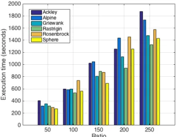
For the first set of experiments all benchmark functions (Section IV-C) were run on the Hadoop cluster. The dimension of the benchmark functions was set to 30, krill population was 50, and the number of iterations was 10,000. Figure 2 shows the result of the experiments. The execution time is plotted against the ratio. The ratio is defined as the number of runs per mapper, i.e., how many independent algorithm runs are completed in one mapper. The figure shows that overall all execution times for all benchmark functions are increasing with increasing ratio values as expected. The largest increases are seen for the Ackley and Alpine benchmark functions, however, all execution times are within a certain range since all benchmark functions are approximately of the same complexity.

Fig. 2. Execution time versus ratio for all benchmark functions with 30 dimensions

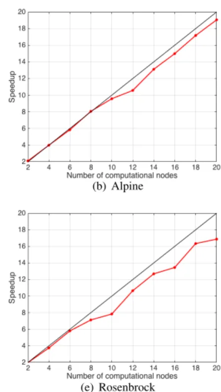
The speedup graphs are given in Figure 3. The speedup is calculated by the ratio of the execution time using one node and the execution time ofn nodes. All speedup figures show the expected trend with the ideal speedup given as the black line. The Alpine benchmark function obtains the best speedup, which is very close to the ideal speedup followed by the Ackley benchmark and Griewank benchmark. However, the remaining benchmark functions also achieve good speedup

TABLE I BENCHMARK FUNCTIONS

Benchmark Mathematical expression Range Objective value

Ackley f(x) =−aexp(−0.02 qPn i=1x2i n )−exp( qPn i=1cos(xi) n +a+ exp(1),a= 20 [-32,32] 0.0 Alpine f(x) =Pn i=1|xisin(xi) + 0.1xi| [-10,10] 0.0 Griewank f(x) =Pn i=1 x2_i 4000− Q cos(√xi i) + 1 [-600,600] 0.0 Rastrigin f(x) = 10n+Pn i=1(x 2 i−10 cos(2πxi)) [-5.12,5.12] 0.0 Rosenbrock f(x) =Pn−1 i=1 100(xi+1−x 2 i)2+ (1−xi)2 [-2.048,2.048] 0.0 Sphere f(x) =Pn i=1x 2 i [-5.12,5.12] 0.0

values. For example using 20 nodes, the highest speedup obtained by the Alpine function is 19.05, and the lowest speedup obtained is 14.86by the Sphere function.

B. Various Dimensions of Alpine Benchmark Function

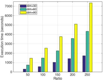
The second set of experiments examines the Alpine bench-mark function for dimensions of 30, 60, and90. Again, the krill population was set to50, and the number of iterations was 10,000. Figure 4 shows the results of running the krill herd algorithm on the Hadoop cluster. As expected, with increasing dimensionality of the Alpine benchmark function increasing numbers of the execution time are observed. For example at ratio 50 the execution times are 315 seconds, 763 seconds, 1,486 seconds for dimensions 30, 60, and 90, respectively. However, the differences between the different dimensions are more visible for the ratio of250were the execution times were 1,737seconds,4,343seconds,7,361seconds for30,60, and 90, respectively.

Fig. 4. Execution time versus varying numbers of dimensions for Alpine benchmark function

C. Objective Value and Execution Time for Varying Krill Size and Iteration Combinations

It has been proven in [23] that the size of the population has a significant effect on the performance of population-based optimization algorithms, even when the total number of function evaluations is kept constant. Thus, the third set of experiments looks at the objective value obtained by the krill herd algorithm as well as the execution time for varying combinations of krill size and number of iterations used. Table II shows the objective value and execution time for the different combinations. The number of function evaluations for each combination was kept constant at half a million. As can be observed from the objective values, the best objective value of 5.738E−08 is obtained for 400 krills and 1,250 iterations. The second best value (2.884E−08) is obtained for a population of300krills and the execution of1,667iterations. The execution times listed in the table are also given as a graph in Figure 5. As expected, it can be observed that the execution time rises for increasing number of krills used. The reason for this is the higher storage requirement of increasing krill populations.

D. Speedup comparing MapReduce-enabled Version with Nor-mal Krill Herd Algorithm Implementation

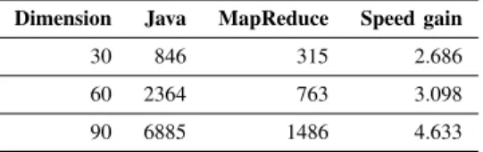
For this experiment we compare the execution time of the krill herd algorithm when run as a non-parallelized Java implementation versus the MapReduce-enabled Java imple-mentation. Fifty runs are executed for both algorithms on the Alpine benchmark function. The fifty runs for the MapReduce-enabled version were executed on two nodes. The speedup is calculated by the ratio of the execution time of the normal krill herd algorithm and the MapReduce-enabled version.

Table III shows the results tabulating the execution time in seconds and the calculated speed gain for the Java imple-mentation (listed as Java) and the MapReduce-enabled Java implementation (listed as MapReduce). The execution time has increased for both versions with increasing dimensionality. The speed gain values achieved for30,60, and90dimensions are 2.686, 3.099, and 4.633, respectively. With increasing dimensionality of the benchmark function, the higher speedup can be obtained. The reason for this is that the MapReduce

(a) Ackley (b) Alpine (c) Griewank

(d) Rastrigin (e) Rosenbrock (f) Sphere

Fig. 3. Speedup for all benchmark functions

TABLE II

OBJECTIVE VALUE ANDEXECUTIONTIME FORVARIOUSNUMBERS OF

KRILL ANDITERATIONCOMBINATIONS FORALPINE WITH30

DIMENSIONS

# krills # iterations Obj. value Exec. time (s)

50 10,000 1.717E-07 315 100 5,000 3.031E-07 435 200 2,500 3.751E-07 671 300 1,667 2.884E-08 966 400 1,250 5.738E-08 1159 500 1,000 3.367E-06 1700

overhead weighs more on the smaller dimensions since they have shorter overall execution times, and thus, better speedup values are obtained for higher dimensions.

VI. CONCLUSION

In this paper, the krill herd algorithm was investigated when run on a Hadoop cluster. The algorithm was parallelized with MapReduce. Four different sets of experiments were conducted to evaluate the krill herd algorithm in terms of speed and accuracy. The experiments were as follows:

• Investigation of the execution time and speedup of the

krill herd algorithm applied to six different benchmark functions;

• Investigation of varying dimensions of the Alpine

bench-mark function with regards to the effect on the execution time;

Fig. 5. Execution time versus various number of krill and iteration combinations for Alpine with 30 dimensions

• Analysis of the effect of different krill sizes and numbers of maximum iterations on the execution time but also on the objective value;

• Comparison of the speedup that can be achieved when

running the MapReduce-enabled version of the krill herd algorithm compared to the java-based krill herd imple-mentation.

The results overall demonstrate that the execution of the krill herd algorithm is particularly useful for higher dimensional

TABLE III

EXECUTION TIME IN SECONDS AND SPEED GAIN OF BOTH

IMPLEMENTATIONS OF THE KRILL HERD ALGORITHM ONALPINE BENCHMARK FUNCTION

Dimension Java MapReduce Speed gain

30 846 315 2.686

60 2364 763 3.098

90 6885 1486 4.633

problems, and thus, achieving very good speedup values. Since the six different benchmark functions are of similar com-plexity, no major differences in execution times can be seen. The best objective value for the Alpine benchmark function using 30dimensions is obtained using400 krills and running the algorithm for 1,250 iterations. However, for the other combinations of krill size and maximum number of iterations, the objective value were close. The last experiment showed that experiments can be run much faster when executed on a Hadoop cluster. In summary, the larger the problem to be optimized (in our case the higher dimensionality), the larger the speedup obtained.

Overall, should a Hadoop cluster be available, then the execution of nature-inspired algorithms on the whole could be performed much faster in particular when large set of experiments and difficult function optimization are involved.

VII. ACKNOWLEDGEMENTS

The author acknowledges the Texas Advanced Computing Center (TACC) at the University of Texas at Austin for providing HPC resources that have contributed to the research results reported within this paper.

REFERENCES

[1] M. Snir, S. Otto, S. Huss-Lederman, D. Walker, J. Dongarra, MPI: The Complete Reference. MIT Press Cambridge, MA, USA. ISBN 0-262-69215-5, 1995.

[2] J. Dean and S. Ghemawat, MapReduce: Simplified Data Processing on Large Clusters, Proceedings of 6th Symposium on Operating System Design and Implementations, USA, 2004.

[3] Apache Software Foundation, Hadoop MapReduce, 2011. http://hadoop. apache.org/mapreduce.

[4] I. Aljarah, S. A. Ludwig, Parallel Particle Swarm Optimization Clustering Algorithm based on MapReduce Methodology, Proceeding of Fourth World Congress on Nature and Biologically Inspired Computing (IEEE NaBIC), Mexico City, Mexico, November 2012.

[5] T. White, Hadoop: The Definite Guide, O’Reilly Media, 2009. [6] J. S. Sarma. Hadoop - Facebook Engg, Note, 2011, http://www.facebook.

com/note.php?noteid=16121578919.

[7] Yahoo Inc. Hadoop at Yahoo! 2011, http://developer.yahoo.com/hadoop. [8] B. Langmead, M. Schatz, J. Lin, M. Pop, and S. Salzberg, Searching for

SNPs with cloud computing, Genome Biol, 10(11):R134, 2009. [9] T. Gunarathne, T. Wu, J. Qiu, and G. Fox, Cloud computing paradigms

for pleasingly parallel biomedical applications, In 19th ACM International Symposium on High Performance Distributed Computing, pages 460-469. ACM, 2010.

[10] S. Krishnan, C. Baru, and C. Crosby, Evaluation of MapReduce for Gridding LIDAR Data, In 2nd IEEE Intl Conf on Cloud Comp Tech and Science, 2010.

[11] M. Stonebraker, The case for shared nothing, Database Engineering Bulletin, 9(1):4-9, 1986.

[12] C. Jin, C. Vecchiola, R. Buyya, MRPGA: An extension of mapreduce for parallelizing genetic algorithms. Proceedings of the 2008 Fourth IEEE International Conference on eScience, Washington, DC, USA, 2008. [13] A. Verma, X. Llora, D. Goldberg, R. Campbell, Scaling genetic

algo-rithms using mapreduce. Ninth International Conference on Intelligent Systems Design and Applications, 2009.

[14] D. W. Huang, J. Lin, Scaling populations of a genetic algorithm for job shop scheduling problems using mapreduce. IEEE Second International Conference on Cloud Computing Technology and Science (CloudCom), 2010.

[15] A. McNabb, C. Monson, K. Seppi, Parallel pso using mapreduce. IEEE Congress on Evolutionary Computation, 2007.

[16] S. A. Ludwig, MapReduce-based Optimization of Overlay Networks using Particle Swarm Optimization. Proceedings of Genetic and Evo-lutionary Computation Conference (ACM GECCO). Vancouver, BC, Canada, 2014.

[17] B. Wu, G. Wu, M. Yang, A mapreduce based ant colony optimization approach to combinatorial optimization problems. Eighth International Conference on Natural Computation (ICNC) pp (728-732), 2012. [18] S. A. Ludwig and D. Dawar, Parallelization of the Enhanced Firework

Algorithm using the MapReduce Framework, International Journal of Swarm Intelligence and Research, IGI Global, vol. 6, no. 2, pp. 32-51, 2015.

[19] N. Al-Madi, I. Aljarah, S. A. Ludwig, Parallel Glowworm Swarm Optimization Clustering Algorithm based on MapReduce: In Proceedings of the IEEE Symposium Series on Computational Intelligence (SSCI). Orlando, USA, 2014.

[20] S. A. Ludwig, MapReduce-based Fuzzy C-Means Clustering Algorithm: Implementation and Scalability, International Journal of Machine Learn-ing and Cybernetics, SprLearn-inger, vol. 6, no. 6, pp. 923-934, 2015. [21] A. H. Gandomi, A. H. Alavi, Krill Herd: a new bio-inspired optimization

algorithm, Communications in Nonlinear Science and Numerical Simu-lation, 17(12):4831-4845, 2012.

[22] J. Marr, The Natural History and Geography of the Antarctic Krill (Euphausia Superba Dana), Discovery Reports 32, 33-464, Cambridge University Press, 1962.

[23] K. M. Malan and A. P. Engelbrecht, Algorithm comparisons and the significance of population size, Evolutionary Computation, 2008.