2009/73
■
Cycle commuting in Belgium:
Spatial determinants and 're-cycling' strategies
Grégory Vandenbulcke, Claire Dujardin, Isabelle Thomas, Bas de
Geus, Bart Degraeuwe, Romain Meeusen and Luc Int Panis
Center for Operations Research
and Econometrics
Voie du Roman Pays, 34
B-1348 Louvain-la-Neuve
Belgium
http://www.uclouvain.be/core
D I S C U S S I O N P A P E R
CORE DISCUSSION PAPER 2009/73
Cycle commuting in Belgium:
Spatial determinants and 're-cycling' strategies
Grégory VANDENBULCKE1, Claire DUJARDIN2, Isabelle THOMAS3,
Bas DE GEUS4 , Bart DEGRAEUWE5, Romain MEEUSEN6
and Luc INT PANIS7
November 2009
Abstract
This paper attempts to explain the spatial variation of the use of a bicycle for commuting to work at the level of the 589 municipalities in Belgium. Regression techniques were used and special attention was paid to autocorrelation, heterogeneity and multicollinearity. Spatial lag models were used to correct for the presence of spatial dependence and a disaggregated modelling strategy was adopted for the northern and southern parts of the country. The results show that much of the inter-municipality variation in bicycle use is related to environmental aspects such as the relief, traffic volumes and cycling accidents. Town size, distance travelled and demographic aspects also have some effect. In addition, there are regional differences in the effects of the structural covariates on bicycle use: the impact of variables such as traffic volume and cycling accidents differs substantially between the north and the south of the country. This paper also suggests that high rates of bicycle use in one municipality stimulate cycling in neighbouring municipalities, and hence that a mass effect can be initiated, i.e. more cycle commuting encourages even more commuters in the area to cycle. These findings provide some recommendations for decision-makers wishing to promote a shift from car to bicycle use.
Keywords: cycling, commuting, spatial lag model, spatial regime, pro-cycling strategies.
1 Université catholique de Louvain, CORE and Department of Geography, B-1348 Louvain-la-Neuve, Belgium. E-mail: Gregory.vandenbulcke@uclouvain.be
2
Université catholique de Louvain, CORE and FRS-FNRS, B-1348 Louvain-la-Neuve, Belgium. E-mail: Claire.dujardin@uclouvain.be
3 Université catholique de Louvain, CORE and FRS-FNRS, B-1348 Louvain-la-Neuve, Belgium. E-mail:
isabelle.thomas@uclouvain.be. This author is also member of ECORE, the association between CORE and ECARES.
4 Department of Human Psychology and Sports Medicine, Vrije Universiteit Brussel, B-1050 Brussels, Belgium. 5Flemish Institute for Technological Research (VITO), B-2400 Mol, Belgium.
6Department of Human Psychology and Sports Medicine, Vrije Universiteit Brussel, B-1050 Brussels, Belgium. 7Flemish Institute for Technological Research (VITO), B-2400 Mol, Belgium and Transportation Research Institute, Universiteit Hasselt, B-3590 Diepenbeek, Belgium. SHAPES Coordinator (SHAPES: Systematic analysis of Health risk and physical Activity associated with cycling PoliciES).
This paper presents research results of the Belgian Program on Interuniversity Poles of Attraction initiated by the Belgian State, Prime Minister's Office, Science Policy Programming. The scientific responsibility is assumed by the authors.
1. Introduction
Most developed countries face environmental and mobility problems as a consequence of widespread car use. Partly due to long-term trends such as the increase in per capita income, car ownership has increased substantially since 1950 (Pooley and Turnbull, 2000; Rietveld, 2001). This has induced many changes, and made our societies more car dependent, leading to the progressive development of new low-density residential estates as well as commercial and industrial activities in peripheral locations (peri-urbanisation). Individuals now have higher levels of mobility and they travel more often, over larger distances, and carry out more complex trips (i.e. they undertake several activities in one trip) (Jensen, 1999; Knowles, 2006). This has various negative impacts upon society and the environment: congestion, air pollution, noise, vibrations, health problems (e.g. due to a lack of physical activity or the inhalation of polluting agents), accidents, growing infrastructure costs, and accessibility problems for low-income groups (Dobruszkes and Marissal, 1994; EC, 2000; Kingham et al., 2001; Bergström and Magnusson, 2003; Witlox and Tindemans, 2004; Knowles, 2006; EEA, 2007).
The promotion of public transport and/or non-motorised modes of transport is intended to address such environmental and mobility problems. More particularly, cycling is a “green” alternative to commuting by car (Chapman, 2007; Woodcock et al., 2007). It is also a space- and energy-efficient mode of transport and is affordable for a large majority of households (Pucher et al., 1999; Rietveld, 2001; Gatersleben and Appleton, 2007; Woodcock et al., 2007). Thus a substantial shift from car to bicycle could reduce urban congestion as well as the environmental harm caused by air and noise pollution. Moreover, cycling to work provides health benefits (if performed on regular basis) (de Geus et al., 2008, 2009) and may help to allay some of the growing concerns about the physical inactivity (which is the second major cause of premature death in industrial countries, after tobacco (BMA, 1992; Pucher et al., 1999; WHO, 2002a, 2002b)).
In Belgium, while approximately 21% of commuters live within cycling distance (i.e. less than 5 km) of their work, and 39% make trips of less than 10 km, only 6% of all commuting trips are carried out with a bicycle as the main method of transport (Verhetsel et al., 2007). The percentage of people who live within 5 km of their work who commute by bicycle is relatively low (19%), and the majority (more than 53%) use their car. There is hence great potential for a shift from car to bicycle for short commutes. However, there are several societal, economic and environmental factors that dissuade people from cycling. These include a lack of cycling infrastructure, the topography, weather, road accidents, and company-related constraints. They need to be clearly identified to help policy makers to mitigate them and to promote bicycle use in Belgium. Such findings could then support the implementation of adequate policies in favour of a modal shift from car to bicycle commuting, at least for short distances.
Within this framework, we aimed to examine which factors have the greatest influence on bicycle use for commuting in Belgium. We therefore carried out multivariate analyses out at the scale of all 589 municipalities (the smallest administrative unit) in the country. A large set of “explanatory” variables was included in the analysis, with specific attention to environmental variables as well as demographic components. Spatial autocorrelation, heterogeneity and multicollinearity problems were diagnosed and treated, with the aim of improving the results.
The structure of the paper is as follows. A thorough review of the literature on the factors that have a potential impact on bicycle use is given in Section 2. The third section presents the spatial context. Section 4 describes the objectives of the paper and the data (dependent variable and explanatory variables) in more detail. The methodological approach used to deal with multicollinearity, heterogeneity and spatial autocorrelation is presented in Section 5. The results of the multivariate analyses are reported in Section 6. Potential pro-cycling strategies are discussed in Section 7, on the basis of the results. Finally, in Section 8, our concluding remarks underscore the importance of accounting for multicollinearity, spatial dependence and spatial heterogeneity to achieve reliable statistical inferences.
2. Identifying the main determinants of bicycle use
A large range of factors have an impact on bicycle use in commuting trips: demographic, socio-economic, societal, cultural, but also environmental and policy-related determinants act as deterrents or encourage cycling. Based on an extensive review of the literature, this section provides a short overview of these determinants.
2.1. Demographic and socio-economic determinants
Socio-economic and demographic determinants include age, income, gender, education, professional field and status, and family commitments (e.g. having young children). Young commuters (< 25 years) generally have low/medium income and often cannot afford a car, which has a clear impact on their choice. Moreover, some of them do not have a driving license and have to use public transport or non-motorised forms of transport when they travel to work. The physical abilities of individuals also depend on their age: young commuters are more likely to enjoy good physical health and to cycle more. Gender has an influence on the decision on whether or not to cycle: on average, men cycle to work more often than women, although women travel shorter distances than men (Ortúzar et al., 2000; Dickinson et al., 2003; Vandenbulcke et al., 2009). Among other factors, women tend to give their personal security as a reason for not using a bicycle, and often make more complex trips than men due to family commitments (Pooley and Turnbull, 2000; Dickinson et al., 2003; Rietveld and Daniel, 2004; Gatersleben and Appleton, 2007).
Education also has a strong influence on bicycle use, but this depends on the area being studied. In North America a high educational level is positively associated with cycling (Noël, 2003; Plaut, 2005; Zahran et al., 2008), whereas the opposite effect is observed in Santiago (Chile) (Ortúzar et al., 2000) and Belgium (Hubert and Toint, 2002). Lastly, the professional field and status play a role (SSTC, 2001; Titheridge and Hall, 2006; Parkin et al., 2008; Heinen et al., 2009). For instance, Pucher et al. (1999) showed that in San Francisco lots of messengers are immersed in a cycling culture and use their bicycles in spite of the hilly topography. Bicycle use for commuting is generally high in academic towns (Martens, 2004; Rodríguez and Joo, 2004).
2.2. Cultural and societal determinants
The literature often mentions that societal and cultural factors influence bicycle use (see e.g. Jensen, 1999; Pucher et al., 1999; Ortúzar et al., 2000; Rietveld, 2001; Dickinson et al., 2003; Rietveld and Daniel, 2004; Plaut, 2005; Pucher and Buehler, 2006; Zahran et al., 2008). A low societal status often tends to be associated with commuter cycling, especially in countries where the car is dominant (e.g. US); utilitarian cycling is often considered as a fringe activity
and suffers from a renegade image (Pucher et al., 1999; Moudon et al., 2005). However, the cycling culture is quite developed in some Northern countries of Europe (e.g. the Netherlands, Sweden, Denmark, Germany and Belgium). Such differences between countries, regions or even ethnicities are probably explained by tradition and lifestyle. A meaningful example is provided by Rietveld and Daniel (2004), who show that immigrants with a different cultural background are unlikely to cycle in the Netherlands and prefer to use public transport or a car.
2.3. Environmental determinants
The main environmental determinants influencing bicycle use are relief, weather (and climatic conditions), urban spatial structure, and infrastructure. Hills influence the attractiveness of non-motorised modes of transport, and there is generally less cycling in hilly areas (Noël, 2003; Rodríguez and Joo, 2004). Cycling up hills is uncomfortable and requires substantial physical effort (Rietveld, 2001; Gatersleben and Appleton, 2007). It also affects travel time in the generalised cost function since it is slower than going down hill or on the flat.
Weather (short-term) and climatic (long-term) conditions are also often mentioned in the literature. Low or high temperatures (e.g. extreme heat combined with air pollution), frequent rain and strong winds may act as deterrents to commuter cycling (Nankervis, 1999; Richardson, 2000; Bergström and Magnusson, 2003; Parkin et al., 2008; Zahran et al., 2008; Koetse and Rietveld, 2009). Like topography, these factors decrease the level of comfort of cycling and increase the physical effort required.
The urban structure influences the likelihood of commuter cycling through several factors, such as population and job densities, mixed land-use and town size (Kitamura et al., 1997; Rietveld, 2001; Vandenbulcke et al., 2009). In urban areas, a high degree of connectivity (i.e. the ability to travel directly), associated with short distances (due to compactness and the presence of mixed-use activities) encourage cycling and walking in commuting trips (Saelens et al., 2003). Distance is an important barrier that limits cycling: only people living close to their workplaces will be interested in cycling (Kingham et al., 2001; Dickinson et al., 2003). Town size also seems to play a key role: few large cities (with more than 2 million inhabitants) have a bicycle commuting rate exceeding 10%. Medium-sized and compact cities perform better since they contain fewer barriers (e.g. motorways) and traffic densities are lower (Pucher et al., 1999). In the largest cities, proximity to the nearest stop and the high frequency of services also make public transport attractive and highly competitive for distances between 1 and 7.5 km. Up to 1 km, walking competes strongly with cycling (Pucher et al., 1999; Ortúzar et al., 2000; Witlox and Tindemans, 2004; Vandenbulcke et al., 2009). Infrastructure (e.g. cycleways and cycle racks) is an essential ingredient for improving bicycle use and cyclists’ safety (Hopkinson and Wardman, 1996; McClintock and Cleary, 1996; Rietveld, 2001). Well-planned and well-kept infrastructure (through design, maintenance and adequate connectivity) encourages cycling and reduces road accidents. Depending on the type of planning, several benefits can be provided for cyclists: e.g. improved comfort, reduced travel time, more enjoyment and increased safety. Dedicated paths (e.g. residential streets) as an alternative to main urban roads are an efficient way of reducing the exposure of cyclists to exhaust fumes (Hertel et al., 2008; Thai et al., 2008). Increased safety can also be achieved by developing continuous and designated cycle lanes, and ensuring that cyclists are still visible to motorists; this is often more highly valued by cyclists than other factors (e.g. reduced travel time, easy parking) (Hopkinson and Wardman, 1996; Tilahun et al., 2007). A well-developed network of cycleways combined with the provision of bicycle parking facilities at
stations/stops may improve the accessibility of public transport to cyclists (Bike-and-Ride), and hence, provide a competitive alternative to the car for commuting trips (Martens, 2004; 2007). Finally, the presence of facilities such as covered/secure cycle parking, lockers, showers and changing facilities at the workplace stimulates commuter cycling (Rietveld, 2000; Kingham et al., 2001; Dickinson et al., 2003; Pucher and Buehler, 2006; Van Malderen et al., 2009). Combined with the provision of continuous cycleways and a mileage allowance for cycling to work, such facilities are expected to have a significant impact on commuting by bicycle (Wardman et al., 2007; Van Malderen et al., 2009).
2.4. Policy-related determinants
Policy-related variables (i.e. planning and pro-cycling policies) play a key role in encouraging more and safer cycling through the implementation of a wide range of measures (Pucher et al., 1999; Rietveld, 2001; Dickinson et al., 2003; Pikora et al., 2003; Pucher and Buehler, 2008). Land-use planning can prevent urban sprawl by favouring compact and mixed-use solutions which reduce travelling distances and – consequently – favour the use of non-motorised transport for commuting (Cervero and Kockelman, 1997; Kitamura et al., 1997; Meurs and Haaijer, 2001; Noël, 2003; Titheridge and Hall, 2006; Chapman, 2007; Woodcock et al., 2007). Moreover, transport planning can modify the design and lay-out of transport networks to improve the connectivity of bikeable roads between different destinations. It can increase the directness of travel through the creation of special intersection modifications for cyclists (e.g. priority signalling), the suppression of barriers (e.g. foot and cycle bridges over waterways and motorways), the creation of detours for car drivers, and the introduction of traffic-calming or car-free zones in urban centres (Meurs and Haaijer, 2001; Rietveld, 2001; Saelens et al., 2003; Pucher and Dijkstra, 2003; Pucher and Buehler, 2006; 2008). This makes cycling safer by reducing the risk of collision with motorised traffic, but also more convenient by allowing cyclists to avoid detours and traffic jams (Rietveld, 2001). Improving safety is of prime importance as it is well-known that the (perceived) risk of death and injury in traffic crashes strongly discourages people from cycling (Hopkinson and Wardman, 1996; McClintock and Cleary, 1996; Curtis and Headicar, 1997; Jacobsen, 2003; Pikora et al., 2003; Pucher and Dijkstra, 2003; Pucher and Buehler, 2006; Parkin et al., 2007). The provision of secure facilities (e.g. guarded cycle racks) along with police surveillance are also efficient means of reducing the risk of bicycle theft or vandalism (which are strong deterrents to cycling).
Financial measures can also promote non-motorised modes of transport and regulate the use of the private car. The provision of monetary incentives such as a mileage allowance or an employer-paid discount on the purchase of a new bicycle may stimulate the practise of commuting by bicycle (Kingham et al., 2001; van Wee and Nijland, 2007; Wardman et al., 2007). For instance, Wardman et al. (2007) showed that a payment of £2 per day could double the level of cycling in Great Britain. Higher parking fees, reduced space for car users (with increased ‘shared space’), fiscal incentives for less polluting cars, higher fuel prices and the implementation of urban tolls (as in London and Stockholm) are some examples of push-measures which can decrease the attractiveness of private car use and encourage a shift to alternative modes of transport (Verhetsel, 1998; van Wee and Nijland, 2007).
Company-related factors can also encourage or discourage commuting by bicycle, especially through their organisational aspects (e.g. a strong dress code, the need to carry bulky goods), location policies, and the availability of facilities (e.g. changing rooms and cycle lockers at the workplace) (Curtis and Headicar, 1997; Dickinson et al., 2003; Heinen et al., 2009). In
particular, a remote location, far from any town or public transport, will result in great dependence on the car and will discourage employees from using any other mode of transport. Employees are also unlikely to travel to work by public transport or bicycle if their company provides free cars and fuel. Only reducing the provision of company cars and fuel, combined with other measures (e.g. incentives for cycling and public transport), can induce a shift away from the car towards alternative modes of transport (Kingham et al., 2001).
Finally, the promotion of cycling is important, since attitudes towards mobility, the environment, etc., are closely linked to travel behaviour (Kitamura et al., 1997). Such promotion can increase cycling and can be achieved through educational programmes (e.g. teaching cycling safety at schools), promotional events, the active involvement of advocacy groups and town officials (e.g. police officers on bicycles), and up-to-date information for cyclists (e.g. cycling maps showing ‘bikeable’ roads) (Curtis and Headicar, 1997; Pucher et al., 1999; Pucher and Buehler, 2006; Zahran et al., 2008). In particular, promotional events can create a mass effect providing cyclists with confidence and enthusiasm (Pucher el al., 1999). Linking cycling to health can also be an efficient way of encouraging more commuters to cycle, since regular exercise improves fitness and health (de Geus et al., 2008; 2009). Cycling is indeed a low-cost way to tackle health problems linked to physical inactivity (e.g. diabetes, cardio-vascular diseases and cancers). It has also been shown to improve mental health and productivity at work (Pucher et al., 1999; EC, 2000; van Wee and Nijland, 2007).
3. Spatial context
The empirical analyses conducted in this paper focus on Belgium, a small and highly urbanised country of more than 10 million inhabitants in a 30,000 km² area. Population densities range from 30 inhabitants/km² in rural regions to more than 20,000 inhabitants/km² in highly urbanised areas. With around 1.5 million inhabitants, Greater Brussels dominates the Belgian town network and is centrally located in the country. Urban sprawl nowadays threatens the quality of life in many Belgian cities. It is at the root of an increased dependence on the car, which causes a large number of negative externalities (congestion, pollution, etc.) (Dobruszkes and Marissal, 1994; Int Panis et al., 2001, 2004).
The popularity of cycling in Belgium is high on average, although far below the levels reported in the Netherlands and Denmark (Witlox and Tindemans, 2004). There has been a substantial decline in the use of bicycles since 1950, as the use of cars for routine trips has increased. The bicycle is now relegated to a marginal role, and is mainly used for recreational activities: indeed, in 2001, only 6.2% of commuters regularly used a bicycle as their main mode of transport (7.4% when bicycles were integrated into a multimodal chain). This compares to 68.6% of commuters who travelled by car (Verhetsel et al., 2007). However, in recent years there have been suggestions that a cycling renaissance is occurring in Belgium, as well as in a number of other European countries (Rietveld, 2001; Witlox and Tindemans, 2004). Furthermore, there are marked differences between Flanders (the northern, Dutch-speaking part of the country) on the one hand, and Wallonia and Brussels (the largely French-speaking southern and central parts) on the other hand. Some 91% of the commuter cyclists live in Flanders, whereas only 6.4% and 2.6% respectively live in Wallonia and Brussels. Several factors – such as cycling policies, culture and topography – are identified in Sections 6 and 7 of this paper to explain this difference.
4. Objectives and data
The main aim of this paper is to explain the variation of the proportion of commuters who travel by bicycle (dependent variable, y), as measured at the scale of the 589 municipalities in Belgium; note that y is continuous, non-negative and constrained to a specific range1. Explanatory variables used in the multivariate analyses fall into three main categories (demographic and socio-economic, policy-related, and environmental) and refer to most of the determinants identified in Section 2. Appendix A lists and describes the explanatory variables. Note that the societal and cultural variables described in Section 2 were not included in this analysis, except through the integration of spatial regimes in the final model2.
Most of the demographic and socio-economic variables come from the 2001 census (a self-administered questionnaire), carried out by the National Institute for Statistics (NIS, 2001b; NIS, 2004)3. The census provides data on individual and household features such as age, gender, level of education, presence of young children in the household, and subjective health which can be aggregated by municipality. Data related to income and car availability were also extracted from the NIS website.
Environmental and policy-related variables come from a wide range of sources. The variables selected for use in this paper not only result from policy decisions (e.g. land-use and transport-related measures), but also characterise the “environment” in which commuters live and travel. Some of these variables (such as population and job densities, average commuting distance, distance to the nearest town, town size, the percentage of commuters living within 10 km of their workplace, the percentages of urban/forest/agricultural land, and the percentage of the land dedicated to public/recreational services) are proxies for the urban structure, land use and accessibility of activities/facilities in the municipality. Others (such as the risk of accidents to cyclists, traffic volumes, the risk of bicycle theft, dissatisfaction with cycling facilities, hilliness, and air pollution) are representative of the overall convenience of cycling in the municipality.
5. Methodology
A combination of exploratory (spatial) data analyses and spatial econometric techniques was employed, using several statistical software packages (SAS, GeoDa and R). Descriptive statistics and bivariate analyses were computed first, to explore the relationships between each of the explanatory variables and the dependent variable y (i.e. the proportion of commuting which is by bicycle). Multivariate models were then applied, with the aim of examining the relative importance of the explanatory variables for the spatial variation in bicycle use (at the scale of municipalities). To improve the statistical inference process, special attention was paid to multicollinearity, spatial heterogeneity (i.e. heteroskedasticity and/or structural instability) and spatial autocorrelation.
1
Linear models could be hence less suited here; however, good results are obtained and suggest that the methodological approach adopted here is quite satisfactory.
2
Exploratory spatial data analyses (ESDA) does indeed suggest that the regimes/clusters defined in Section 5 are representative of different cultures (the Flemish-Walloon split).
3
The census is preferred to other surveys (e.g. NIS, 2001a) since it is the most recent database and covers the entire population.
5.1. The validity of the ordinary least squares model
The first step in testing the validity of the ordinary least squares (OLS) model was to compute condition indices, tolerance and variance inflation factor (VIF) values so as to diagnose the existence of multicollinearity. The major assumptions of the regression (linearity, homoscedasticity, normality and spatial independence of the residuals) were then tested. The White, Breusch-Pagan and Koenker-Bassett tests for the presence of heteroskedasticity were performed first, and the asymptotic version HC3 of the heteroskedasticity-consistent covariance matrix (HCCM) was then used to correct for heteroskedasticity (Long and Ervin, 2000). Lagrange multiplier (LM) diagnostics and their robust forms (Robust LM) were preferred to Moran’s I, because they help to identify the form of spatial dependence (spatial error or spatial lag) and because Moran’s I is inappropriate in the presence of heteroskedastic or non-normally distributed errors (Anselin and Rey, 1991; Anselin and Florax, 1995; Anselin et al., 1996; Anselin, 2005). Finally, the Jarque-Bera statistic was used to test the assumption of normality.
5.2. Spatial autoregressive modelling
Spatial autoregressive modelling (SAR) was used to deal with the presence of spatial autocorrelation. It is divided into two alternative specifications: spatial error and spatial lag models. While the first specification suggests the presence of omitted explanatory variables, the second indicates the possibility of a diffusion process (i.e. an event in one municipality increases the likelihood of the same event occurring in neighbouring municipalities).
The spatial error model (SEM) specifies a spatial autoregressive process for the error term
ε
to account for the spatial influence of unmeasured (or omitted) explanatory variables on the proportion of commuting by bicycle in neighbouring municipalities. For N observations and K exogenous independent variables, the structure of the SEM in matrix form is:ε
β
+= X
y (1)
with
ε
=λ
Wε
+ξ
(2)where y is a N × 1 vector of observations i of the dependent variable (proportion of commuting by bicycle in municipality i),
β
is a K × 1 vector of coefficients of the independent variables, X is a N × K matrix of observations i of the independent variables (including a constant term),ε
is a N × 1 vector of error terms at location i,λ
is a spatial autoregressive coefficient, W is a N × N spatial weights matrix (row-standardised) andξ
is a white noise error. In this study, N = 589 (the number of municipalities in Belgium).By contrast, the spatial lag model (SLM) assumes that the dependent variable in municipality i is influenced by the values of the dependent and independent variables in the surrounding municipalities j. The magnitude of this spatial influence (or “spillover effect”) is captured by a spatial autoregressive coefficient
ρ
. In matrix notation, the SLM specification is:ε
β
ρ
+ += Wy X
y (3)
where Wy is the spatially lagged endogenous variable.
Note that for both specifications (lag and error), the standard R² is invalid since a maximum likelihood (ML) estimation is used. Some more appropriate measures of fit are the
log-likelihood, the Akaike information criterion (AIC) and the Schwarz information criterion (SIC) (Anselin, 1988; Anselin, 2005). The validity of the White and Breusch-Pagan tests is also strongly affected when the error terms are spatially correlated (Anselin, 1988). Two alternative tests are hence preferred: the joint LM test and the spatial Breusch-Pagan test. Further details are provided by Anselin (1988), Anselin and Griffith (1988), Le Gallo (2004) and Bivand (2008) about these tests.
5.3. Spatial heterogeneity
Spatial heterogeneity was taken into account in a number of ways. These include focusing on the issue of heteroskedasticity (see Sections 5.1 and 5.2), and testing for the structural stability of coefficients between spatial subsets of the data (spatial regimes). In the presence of structural instability, the parameter estimates take on different values in distinct geographic areas. Formally, a regression with Regimes 1 and 2 (e.g. north and south) is called a spatial regime regression and is expressed as:
+ = 2 1 2 1 2 1 2 1 X 0 0 X y y
ε
ε
β
β
(4)where y1 and y2 are the vectors of observations of the dependent variable,
β
1 andβ
2 are thevectors of coefficients of the independent variables, X1 and X2 are the matrices of observations
of the independent variables (including a constant term for each regime), and
ε
1 andε
2 are thevectors of error terms for Regimes 1 and 2 respectively.
If spatial dependence persists after the spatial heterogeneity has been modelled, the spatial regime specification (4) should also account for spatial autocorrelation. Equation (3) hence takes on the form:
Regime 1: y1 =
ρ
W1y1 +X1β
1 +ε
1 (5) Regime 2: y2 =ρW2y2 +X2β2 +ε2 (6) where W1 and W2 are the spatial weights matrices for Regimes 1 and 2 (Le Gallo, 2004;Anselin, 2007; Bivand, 2008).
5.4. Diagnostics for structural instability
The stability of the coefficients across regimes can be diagnosed using the spatially adjusted version of the Chow test, i.e. the spatial Chow test (CG) (Anselin, 1988). It can also be
detected and visualised using an exploratory spatial data analysis (ESDA). This helps to identify the presence of global and local patterns of spatial autocorrelation and heterogeneity (e.g. spatial outliers or clusters) in the proportion of commuting by bicycle (Anselin, 1998a; 1998b; Le Gallo and Ertur, 2003; Baller et al., 2001; Ramajo et al., 2008). ESDA can be undertaken by performing common measures of spatial autocorrelation, such as the Moran’s I statistic, the Moran scatterplot and the local indicators of spatial association (LISA) (Anselin, 1995; Le Gallo, 2004).
In particular, the Moran scatterplot allows the local spatial association (between a municipality and its neighbours) to be categorised into four groups: HH (municipality with a high value surrounded by municipalities with high values), LH (low value surrounded by high values), LL (low value surrounded by low values) and HL (high value surrounded by low
values). HH and LL refer to spatial clusters (positive spatial autocorrelation), while LH and HL indicate to spatial outliers (negative spatial autocorrelation). Finally, the information derived from the categorisation into four groups, combined with that resulting from the computation of the significance values of LISA yields the LISA cluster map. This gives an indication of the location of significant spatial clustering and diagnoses local instability (e.g. pockets of non-stationarity). It hence facilitates the identification of spatial outliers and spatial regimes (Le Gallo and Ertur, 2003; Baller et al., 2001).
6. Results
6.1. Basic statistics and bivariate correlations
Appendix B presents some basic statistics and shows that most of the explanatory variables are significantly correlated with the dependent variable (with the expected signs). The highest correlations are observed for the variables measuring dissatisfaction with cycling facilities (–0.82), slope (–0.77), bad health (–0.58), young workers (0.54) and long commuting distances (–0.54). Other variables which are negatively correlated with commuting by bicycle are the proportion of working households with young children (–0.39), middle-aged workers (–0.39), forests (–0.33) and the risk of accidents to cyclists (–0.32). Conversely, the density of jobs (0.38), urbanisation (0.34), and traffic volume on regional roads (0.31) all have positive spatial correlations with cycle commuting. Most of these relationships confirm the hypotheses about transport-choice processes set out in Section 2. The positive correlation with traffic volumes is the only anomaly, which is probably explained by the high proportion of cyclists in urbanised areas (where traffic congestion is also high).
6.2. Diagnostics (OLS)
A multivariate regression was first applied using OLS estimation and paying special attention to the heteroskedasticity and multicollinearity issues. The analysis of condition indices, tolerance and VIF values is helpful to lower multicollinearity as much as possible. The Breusch-Pagan and White tests for heteroskedasticity (Table 1) reveal the presence of non-constant error variance in the model; this was corrected using White’s correction (HC3). Results for the White-corrected OLS estimation are reported in Table 2, and indicate quite high goodness-of-fit (R² = 0.879). Most of the parameters are significant at least the 10% level of probability.
The diagnostics in Table 1 (Moran’s I, LM and joint LM tests) do, however, show the presence of spatial dependence, which affects the validity of the OLS estimations. The analysis of the significance of the robust and non-robust forms of the LM tests indicates that the spatial lag model is a better way of addressing the spatial autocorrelation issue.
6.3. Choice of the spatial weight matrix
The computation of a spatial autoregressive model requires the definition of a spatial weight matrix. Here, a “queen” contiguity-based matrix (first order of contiguity; row-standardised) is used because it provides the best fit and results in a model satisfying to the finite sample condition (Wald test ≥ likelihood ratio ≥ Lagrange multiplier) (Anselin, 1988). In the queen case, the elements wij of the weights matrix W are equal to 1 when the municipalities have
6.4. Spatial lag results
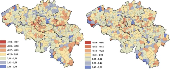
The results for the spatial lag models are presented in Table 2. White’s correction is again used to treat the model for the presence of heteroskedasticity. As the significant Jarque-Bera statistic in Table 1 suggests, the ML estimation is valid since the error terms are normally distributed. The same is true for the LM tests and Moran’s I statistics. The spatial lag model gives a better fit than OLS: the log likelihood statistic increases from –102.4 to 33.7 (Table 2). Moreover, the Moran’s I and the LM test statistics both indicate that including a spatially lagged variable in the model eliminates spatial dependence. This is confirmed by Figures 1a and 1b, which show the spatial autocorrelation of errors to be substantially less in the ML estimation than in the OLS model. This reduction translates into fewer spatial concentrations of similar residuals. The example of Brussels and its periphery is a good example of this: similar OLS residuals are spatially concentrated (Figure 1a), but the ML residuals (Figure 1b) are much less so.
Figures 1a and 1b: OLS (left) and ML residuals (right). The Brussels-Capital Region is centrally located on these maps (see Figure 2). Moran’s I = 0.34 and is significant.
Table 2 shows that the spatial autoregressive coefficient
ρ
(or lag coefficient) is highly significant. This is suggestive of the fact that spillover influences exist between one municipality i and its neighbourhood: the likelihood of cycling in i is (positively) linked to bicycle use in the neighbouring municipalities j. The significance and magnitude of all the regression coefficients are lower for the ML estimation than for OLS, which can be explained by the introduction ofρ
. This suggests that part of the explanatory power of variables in municipality i may really be due to the influence of the neighbouring municipalities j (which is picked up byρ
). Among the significant coefficients, the average change in relative value is high (47%) and illustrates the substantial bias of the OLS model coefficients when spatial dependence is ignored.OLS ML
Diagnostics for normality
Jarque-Bera test 4,62 -
Diagnostics for multicollinearity
Variance Inflation Value (max. value) 3,30 - Condition index (intercept adjusted) 5,03 -
Diagnostics for heteroskedasticity
Koenker-Bassett test 2 28,32** 28,82***
White test 213,64*** -
Breusch-Pagan test (North-South)3 88,68*** 25,08***
Diagnostics for spatial dependence
Moran's I of residuals4 0,34*** 0,01
Lagrange Multiplier (lag) 253,37*** -
Robust LM (lag) 86,74*** -
Lagrange Multiplier (error) 181,96*** -
Robust LM (error) 15,33*** -
Diagnostic for spatial dep. and heteroskedasticity
Joint test LM 213,29*** -
Tests on overall stability
Chow structural instability test5 14,20*** 120,49***
Diagnostics for residual autocorrelation
LM test - 0,00
*Significant at the 90% level **Significant at the 95% level ***Significant at the 99% level n.a.: no test available
1
The spatial Breusch-Pagan test was used for the ML estimation
2
The spatial Koenker-Bassett test was used for the ML estimation
3
Inference computation based on 9999 permutations (for ML estimation only)
4
The spatial Chow structural instability test was used for the ML estimation Table 1: Regression diagnostics for the OLS and ML estimations
OLS, with heterosk. correction ML, with heterosk. correction Intercept 6,4124*** 3,2698*** [0,0000] [0,0000] Lag coefficient (ρ) - 0,6015*** - [0,5483] Demographic variables Working men 0,0472*** 0,01673** [0,1150] [0,0408] Age 2 (45-54 years) -0,0460*** -0,02505*** [-0,1352] [-0,0737] Age 3 (> 54 years) -0,2054* -0,14503* [-0,0456] [-0,0322] Young children -0,0567*** -0,0218*** [-0,1865] [-0,0716] Socio-economic variables
Education 3 (higher/university degree) -0,4988*** -0,23034***
[-0,1261] [-0,0582]
Income 0,0030 0,00852
[0,0072] [0,0206]
Bad health -0,0521*** -0,0189***
[-0,3124] [-0,1133]
Environmental and policy-related variables
Commuting distance -0,0114*** -0,00652**
[-0,0789] [-0,0450]
City size -0,0954*** -0,0875***
[-0,1750] [-0,1604]
[-0,1341] [-0,0683]
Slopes -0,4873*** -0,1763***
[-0,2655] [-0,0961]
Cycling facilities unsatisfaction -0,0127*** -0,0049***
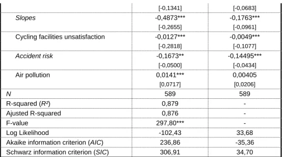
[-0,2818] [-0,1077] Accident risk -0,1673** -0,14495*** [-0,0500] [-0,0434] Air pollution 0,0141*** 0,00405 [0,0717] [0,0206] N 589 589 R-squared (R²) 0,879 - Ajusted R-squared 0,876 - F-value 297,80*** - Log Likelihood -102,43 33,68
Akaike information criterion (AIC) 236,86 -35,36 Schwarz information criterion (SIC) 306,91 34,70
*Significant at the 90% level **Significant at the 95% level ***Significant at the 99% level - : variable not included in the model
Standardized regression coefficients in brackets Italic: variables logarithmically transformed
Table 2: Regression coefficients for the OLS and ML estimations
The signs of the regression coefficients in Table 2 are the same for the OLS and ML estimations. As expected, most of the (significant) explanatory variables introduced in the models have a deterrent effect on the proportion of commuters cycling. Municipalities with high proportions of working people over 45, working households with one or more young children, or inhabitants in poor health have lower levels of commuter cycling. Municipalities characterised by large numbers of highly-educated people also have lower levels of commuter cycling, which confirms the results of previous studies in Belgium (SSTC, 2001; Hubert and Toint, 2002). On the other hand, high levels of cycling are observed in municipalities with high proportions of working men. Among the environmental and policy-related variables, the presence of high accident risks, heavy traffic volumes and steep slopes along the road network are associated with a low propensity to cycle to work. The size of the town also matters, and this is probably associated with the provision of good facilities for cycling. The proportion of commuters cycling is highest in the cities (well-equipped municipalities), and lowest in small municipalities (Vandenbulcke et al., 2009).
Note finally that, when the regression is carried out on the proportion of cyclists among commuters who travel less than 10 km (in municipality i), the results (not shown here) are basically similar to those shown in Table 2. The main difference lies in the variable referring to commuting distances: for commuting trips of up to 10 km, increasing distance is linked to more cycling, whereas in the general regression (Table 2) increasing distance is linked to less cycling. Cycling is a very convenient mode of transport for distances between 2 and 5 km, but for shorter distances (0–2 km) walking is the preferred mode of transport (Vandenbulcke et al., 2009). This suggests that, up to 10 km, commuting distance does not act as a strong deterrent to cycling. Given that approximately 39% of commuters (and even more in urban areas) live less than 10 km from their work, there is considerable potential for a shift to cycling.
6.5. Accounting for spatial heterogeneity
6.5.1. Diagnostics: Chow tests and exploratory spatial data analyses (ESDA)
Structural instability is detected by the Chow test and its spatial extension. Both tests are highly significant and hence clearly reject the null hypothesis of parameter stability. This suggests that the spatial lag results (Table 1) do not completely account for spatial heterogeneity. ESDA techniques confirm these findings and help to identify spatial regimes. The global spatial autocorrelation for the proportion of commuters cycling was first tested using the Moran’s I statistic. This indicated the presence of a positive and significant spatial autocorrelation (I = 0.90; p = 0.0001), which means that municipalities with high rates of cycle commuting are generally located close to other municipalities with high rates (and similarly municipalities with low rates are located close to other municipalities with low rates).
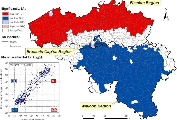
The Moran scatterplot and the LISA cluster map for the dependent variable in Figure 2 help us to identify spatial regimes. The results of the Moran scatterplot suggest the presence of spatial heterogeneity in the form of two distinct spatial regimes, in quadrants I and III. The LISA cluster map illustrates the spatial pattern of these regimes and reveals a clear-cut north/south division of the municipalities: most of the northern municipalities (Flanders) fall into quadrant I, while a large proportion of the southern municipalities (Wallonia and Brussels) fall into quadrant III.
Figure 2: Moran scatterplot and LISA cluster map for the spatial clustering of commuting by bicycle
6.5.2. Spatial regime regression with a spatially lagged variable
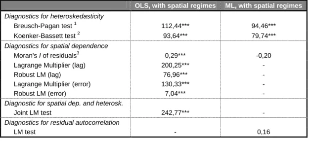
The northern and southern spatial regimes were incorporated into the regression to adjust for spatial heterogeneity. The diagnostics in Table 3 show the existence of spatial autocorrelation and heteroskedasticity in the models. This was corrected by applying an ML estimation (lag)
and a White’s correction (Table 4). The spatial regime specification (with spatial lag) gives a considerably better fit than the spatial lag model, with a log likelihood statistic as high as 93.9 (Table 4).
OLS, with spatial regimes ML, with spatial regimes
Diagnostics for heteroskedasticity
Breusch-Pagan test 1 112,44*** 94,46***
Koenker-Bassett test 2 93,64*** 79,74***
Diagnostics for spatial dependence
Moran's I of residuals3 0,29*** -0,20
Lagrange Multiplier (lag) 200,25*** -
Robust LM (lag) 76,96*** -
Lagrange Multiplier (error) 130,33*** -
Robust LM (error) 7,04*** -
Diagnostic for spatial dep. and heterosk.
Joint LM test 242,77*** -
Diagnostics for residual autocorrelation
LM test - 0,16
*Significant at the 90% level **Significant at the 95% level ***Significant at the 99% level - : no test available
1
The Spatial Breusch-Pagan test is used for the ML estimation
2
The Spatial Koenker-Bassett test is used for the ML estimation
3
Inference computation based on 9999 permutations (for ML estimation only)
Table 3: Regression diagnostics for the OLS and ML estimations, including the spatial regimes
The results in Table 4 show that several explanatory variables are significant for the north (Flanders) but not for the south (Wallonia and Brussels), and vice versa. The signs of the significant coefficients are the same as in the spatial lag specification, but the magnitude differs greatly in some cases. For Flanders, the average change in the (relative) values ranges from 6.4% for dissatisfaction with cycling facilities to 426.5% for the accident risk. For Wallonia and Brussels, this change is less pronounced, ranging from 2.7% for the risk of an accident, to 58.7% for town size. These findings not only illustrate how biased the estimates are when the structural instability is ignored, they also show the substantial difference in the size of these estimates between the Belgian regions. The “accident risk” variable is probably the best example of this.
ML, with spatial regimes and heteroskedasticity correction
North South Intercept 2,3084* 4,3095*** [0,0000] [0,0000] Lag coefficient (ρ) 0,5362*** [0,5097] Demographic variables Working men 0,0296** 0,0008 [1,0246] [0,0288] Age 2 (45-54 years) -0,0417** -0,0205*** [-0,5854] [-0,3007] Age 3 (> 54 years) -0,1074 -0,0680 [-0,1317] [-0,0867]
Young children -0,0365*** -0,0247***
[-0,4372] [-0,3306]
Socio-economic variables
Education 3 (higher/university degree) -0,0968 -0,3132***
[-0,2104] [-0,6862]
Income 0,0311* -0,0027
[0,3824] [-0,0307]
Bad health -0,0098 -0,0146**
[-0,1274] [-0,2481]
Environmental and policy-related variables
Commuting distance -0,0165*** -0,0047* [-0,2061] [-0,0765] City size -0,1146*** -0,0361*** [-0,4539] [-0,1483] Slopes -0,1931** -0,1972*** [-0,1145] [-0,1966]
Cycling facilities unsatisfaction -0,0052*** -0,0045***
[-0,1666] [-0,2227]
Accident risk -0,7632*** -0,1489***
[-0,1047] [-0,0493]
Air pollution 0,0138*** -0,0054
[0,2551] [-0,0956]
Traffic volume 2 (municipal network) -0,2357 -0,4521**
[-0,0306] [-0,0700]
N 589 (NNorth = 308; NSouth = 281)
Log Likelihood 93,923
Akaike information criterion (AIC) -123,846
Schwarz information criterion (SIC) 16,264
*Significant at the 90% level **Significant at the 95% level ***Significant at the 99% level
Standardized regression coefficients in brackets Italic: variables logarithmically transformed
Table 4:Regression coefficients for the spatial regime specification (ML estimation)
6.5.3. Regional variation and the relative importance of the variables
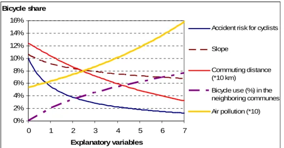
Table 4 suggests that variables such as median income and the proportion of working men are not significantly related to the rate of cycle commuting in Wallonia and Brussels; on the other hand, they are positively related to the rate in Flanders. The positive association between median income and bicycle use can probably be explained by the fact that lower median income is a proxy for crime and vandalism (Parkin et al., 2008). This suggestion is supported by a significant correlation of –0.20 between the median income and the number of bicycle thefts in a municipality (and a correlation of –0.27 between median income and the risk of bicycle theft). The relationship between cycle commuting and the air pollution (the annual mean concentration of PM10s) was also only significant in Flanders. Surprisingly, Figure 3 shows that, on its own, an increase in the PM10 concentration actually increase the rate of cycle commuting in a Flemish municipality: for instance, an increase from 25 to 30 µg/m³ is linked to an increase in the proportion of commuting by bicycle of 8.1%. This is probably explained by the fact that the health risks of air pollutants are not really perceived as barriers to cycling (since cycling is seen as beneficial for health, despite the increased exposure).
Moreover, it suggests that commuter cycling is more common in industrial and/or congested urban environments (which are generally areas with high concentrations of PM10s).
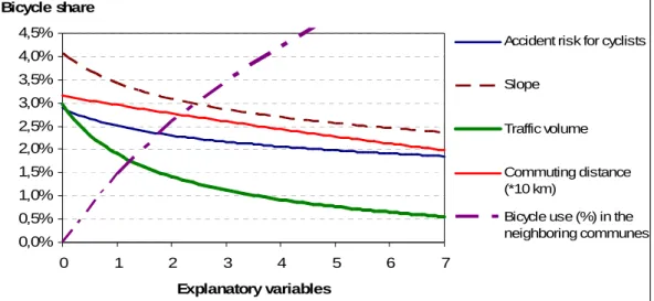
Table 4 shows that three variables which are not significantly related to bicycle use in Flanders do appear to have an impact in Wallonia and Brussels (the southern part of Belgium). The results suggest that a one percentage point decrease in the proportion of inhabitants reporting bad health will increase bicycle use by 0.07%. Relatively good physical and mental health is indeed required to use a bicycle. Moreover, a decrease from 25 to 15% in the proportion of highly qualified people in a municipality is linked to a 17.8% increase in commuter cycling4. Commuters with better qualifications generally get higher wages and fringe benefits such as a company car; this probably explains why they are more likely to have a car at their disposal, and so choose to live far from their workplace, beyond “cycling distance”. Finally, a reduction in the volume of motorised traffic is expected to encourage cycling: a decrease from 200,000 to 100,000 vehicle-km per kilometre of local road per year is predicted to increase bicycle use by 5.23% (Figure 4). Concretely, such a reduction corresponds to a 1,700-km decrease in the mileage of motorised vehicles per municipality per year, or a 4.6-km decrease in the daily mileage5. Ideally, a substantial reduction in traffic, from 1,000,000 to 10,000 vehicle-km (achieved, for example, through the implementation of an urban toll in the municipality) could increase bicycle use by as much as 32%.
0% 2% 4% 6% 8% 10% 12% 14% 16% 0 1 2 3 4 5 6 7 Explanatory variables Bicycle share
Accident risk for cyclists
Slope
Commuting distance (*10 km)
Bicycle use (%) in the neighboring communes Air pollution (*10)
Figure 3: Variation in bicycle use in Flanders as explanatory variables change. Note: these graphs are constructed by varying one explanatory variable, while holding all the others constant at their means (see Rodríguez and Joo, 2004). For ease of illustration, all the explanatory variables are all presented on the same x-axis. Given that the validity of the results may be affected by the presence of feedback effects in the model (LeSage and Fisher, 2008; LeSage and Pace, 2009), we compared the parameter estimates in Table 4 with scalar summary impact measures and observed that feedback effects are quite weak. As a result, the parameter estimates give a reasonable measure of the direct impact of changes (in explanatory variables) on cycling levels in i.
4
Note that this result holds for Wallonia, but does not really applies to Brussels, where most commuter cyclists (66%) are highly qualified. Such a result is explained by the greatest weight of the Walloon municipalities (262 municipalities, compared with the 19 Brussels municipalities).
5
Assuming a 169-km local road network and 10,000 motorised vehicles using this network each year. These figures are based on the averages for Belgian municipalities.
0,0% 0,5% 1,0% 1,5% 2,0% 2,5% 3,0% 3,5% 4,0% 4,5% 0 1 2 3 4 5 6 7 Explanatory variables Bicycle share
Accident risk for cyclists
Slope
Traffic volume
Commuting distance (*10 km)
Bicycle use (%) in the neighboring communes
Figure 4:Variation in bicycle use in Wallonia and Brussels as explanatory variables change. Note: these graphs are constructed by varying one explanatory variable, while holding all the others constant at their means (see Rodríguez and Joo, 2004). For ease of illustration, all the explanatory variables are all presented on the same x-axis. Given that the validity of the results may be affected by the presence of feedback effects in the model (LeSage and Fisher, 2008; LeSage and Pace, 2009), we compared the parameter estimates in Table 4 with scalar summary impact measures and observed that feedback effects are quite weak. As a result, the parameter estimates give a reasonable measure of the direct impact of changes (in explanatory variables) on cycling levels in i.
Most of the other explanatory variables shown in Table 4 have significant relationships with bicycle use in both regions. At first glance, variables such as the proportion of households with young children, or the proportion of commuters aged 45 to 54, seem to be strong deterrent factors for cycling. Their impact is also pronounced in Flanders, than in Wallonia and Brussels. Combined with the results of a principal component analysis (orthogonal varimax rotation; results not reported here), these findings also suggest that: (1) being young (i.e. less than 25 years of age) and having poor qualifications increases the propensity to cycle to work; (2) having more than one young child in the household increases the probability of owning a car, and consequently decreases the likelihood of cycling.
Table 4 also shows the impact town size and dissatisfaction with cycling facilities have on cycle commuting. In both regions, a 10% increase in the proportion of household which express dissatisfaction with the facilities for cycling would reduce bicycle use by about 5.5%. Living in a poorly-equipped municipality (in terms of facilities) is associated with a lower likelihood of using a bicycle, whereas larger towns have a higher proportion of cycle commuting. In Flanders, the largest cities (H1 to H3) score well with cycle commuting rates
31.3 to 58.5% higher than in the most rural municipalities (H6 to H8). In Wallonia and
Brussels, this difference is less pronounced, and only ranges from 3.4 to 9.7%.
Last but not least, Figures 3 and 4 suggest that a high risk of accidents, long commuting distances and hilly terrain decrease the propensity to cycle. Although it is basically similar in the two regions, the impact of the topography on bicycle use is slightly greater in the southern part of the country. An increase of the mean slope of the road network from 1 to 2° (which might occur, for example, when commuters are forced to take an alternative route, due to roadworks or deviations) could reduce the number of commuting cyclists by more than 8.4% in Flanders and 9.9% in Wallonia and Brussels. Conversely, reducing the slopes would significantly increase bicycle use, especially in municipalities where the mean slope is 1 to 2°. Above this “limit”, the impact of a change in the mean slope is lower. The risk of accidents
also strongly discourage bicycle use. In Flanders, an increase in this risk from 0.0 to 0.5 (which corresponds to two more victims per year and per 100,000 bicycle-minutes) is linked to a 29.3% reduction in the number of commuter cyclists. In Wallonia and Brussels, the accident risks is also negatively linked to bicycle use, but to a lesser extent: the same increase in risk (from 0.0 to 0.5) is linked to a fall in bicycle use of only 7.9%. Longer commuting distances have a deterrent effect and do not stimulate cycling. In Flanders, an increase in the average commuting distance from 5 to 15 km would produce a 16.6% decrease in commuter cycling. The same increase in commuting distance in Wallonia and Brussels would reduce the bicycle use by 6.1%. Given that the “commuting distance” variable partly synthesises proximity-related information (through variables such as population and job densities, and urbanised areas)6, it implies that compact environments and tight town networks are associated with low commuting distances and hence stimulate cycling.
6.5.4. Spatially lagged variable
Table 4 shows that the coefficient
ρ
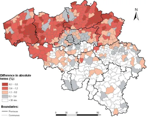
is still highly significant and positive for the spatial regime model. This indicates the presence of a strong diffusion process between neighbouring municipalities: the (neighbouring) municipalities j exert a positive spillover effect on the propensity to cycle in municipality i, which in turn (after t years) could generate a feedback effect on bicycle use in j. In the long-term, such a continuous diffusion process could initiate a “mass effect”, in the form of a virtuous circle which maintains the propensity to use a bicycle for commuting in the region. The municipalities in Wallonia and Brussels seem to be prone to a large reduction in bicycle use if cycling becomes less popular in neighbouring municipalities (and conversely), but Flemish municipalities are more resistant (relatively to Wallonia and Brussels) to the possibility of a fall in bicycle use in surrounding municipalities.Figure 5: Percentage changes (in absolute values) in cycle commuting between 1991 and 2001 Source: Verhetsel et al. (2007)
6
As suggested by Figures 3 and 4, the spillover effect is most pronounced when municipality i and its neighbouring municipalities j all have low rates of cycle commuting: for instance, when the spatially lagged variable Wy is lower than 5%, bicycle use in municipality i still increases but to a lesser extent. Such diffusion processes can be observed in reality, which reinforces the validity of the model. Figure 5 shows that the changes in bicycle use in Belgium between 1991 and 2001 were spatially clustered. For instance, there was an increase in bicycle use in Brussels and its neighbourhood during this period, but the opposite was true in several groups of municipalities in the western and north-eastern parts of the country. 6.5.5. Analysis of the residuals
The residuals of the final specification (Table 4) are mapped in Figure 6. This provides a useful tool for planners and policy makers since it pinpoints both the municipalities that ‘over-perform’ in terms of bicycle use and those where there is still potential to develop the use of the bicycle for commuting trips further. This potential exists in the municipalities characterised by negative residuals (predicted values > observed values). Given the current environment and neighbourhood7, such municipalities could perform better in terms of bicycle use but, for something (e.g. an inadequate or unambitious cycling policy, high-quality public transport, a multicultural town8) holds it back. Examples of municipalities with negative residuals are Antwerp, Brussels, Genk, Ghent and Kortrijk (Courtrai). The last two are surprising, in view of their pro-cycling policies and relatively high rates of cycle commuters, but suggest that there is still potential to encourage more people to cycle to work.
Figure 6: The residuals of the spatial regime specification (see Table 4)
7
The “neighbourhood” here refers to the region (Flanders or Wallonia and Brussels) in which municipality i is located, and the rate of cycling in the neighbouring municipalities j.
8
Immigrants and inhabitants with a foreign background have different cultural reference points, and are generally less likely to cycle (public transport and/or the car are preferred to the bicycle) (Rietveld and Daniel, 2004). In municipalities with a high proportion of foreigners (e.g. Ghent, Brussels, Antwerp), bicycle use is generally lower than in other municipalities with the same environmental features.
At the other end of the scale, positive values of the residuals mean that the observed rate of commuter cycling is higher than predicted by the model. Municipalities characterised by positive values excel in terms of bicycle use (given their environment). The examples of Louvain and Bruges are important in this respect, since they have more pro-cycling policies (in terms of engineering, traffic education and enforcement) than other Flemish municipalities. Several municipalities in Wallonia (e.g. Mouscron, Perwez, Hotton) also perform better than expected, despite their low absolute rates of cycle commuting. Given their environment (steep slopes, rural setting , etc.), they “over-perform”, for example by adopting mobility strategies that encourage bicycle use (SPW, 2008).
7. Discussion and re-cycling strategies
7.1. Socio-economic variables: education, promotion and training
Income, age and gender all have a significant impact on the rate of cycle commuting in Flanders: low median income, low proportions of working women, and a young (under 45) workforce are all associated with high rates of cycling to work. Having one or more young children (0–5 years old) in the household decreases the likelihood of cycling to work in both regions. The presence of many highly-qualified people also matters, particularly in the province of Walloon Brabant. Highly qualified commuters living in Wallonia generally have high incomes, can afford a car, and use it to travel large distances9. They are hence less likely to use a bicycle for their commuting trips (Jensen, 1999).
Promotional and educational campaigns (focused on, for example, health benefits or the possibilities of bike pooling10) could be helpful in addressing some of these socio-economic issues (Pucher and Dijkstra, 2003). Public and private companies should promote existing alternatives to the car, and try to make them competitive by providing financial incentives such as a mileage allowance or a company bicycle.
7.2. Environmental variables: towards optimal paths?
Flat terrain, high-quality cycleways and a low risk of accidents can encourage commuter cycling in both regions. However, heavy traffic (on municipal roads) does not have any significant impact in Flanders, whereas it strongly discourages cycling in Wallonia and Brussels. In Flanders, the high visibility of cyclists in the traffic (because there are such a lot of them) and the presence of appropriate cycling infrastructure probably give commuter cyclists a feeling of personal security and, hence, offset the deterrent effect of traffic volume. Policies in Flanders do indeed provide high-quality infrastructure (e.g. continuous and separate cycleways) and facilities (e.g. changing facilities at work, covered cycle racks) with the intention of improving the safety and convenience of cycling. Flanders also stimulates bicycle use through regulations restricting motorised traffic in urban centres (e.g. through the introduction of traffic calming areas), so that the risk and annoyance of heavy traffic is greatly reduced. Finally, motorists show more respect for cyclists because they often cycle themselves and/or are used to sharing the road with large numbers of cyclists.
The opposite situation is observed in Wallonia and the Brussels region: here, the terrain is more hilly and discourages cycling. Also, motorists are seldom mindful of commuter cyclists
9
Commuters with a car at their disposal and attracted by green amenities often try to live on the outskirts of large cities. Public transport in these areas is often poor, and so long commuting journeys by car are common.
10