TÜS
İ
AD-KOÇ
UNIVERSITY ECONOMIC RESEARCH FORUM
WORKING PAPER SERIES
PROVISION OF LIQUIDITY THROUGH THE PRIMARY CREDIT
FACILITY DURING THE FINANCIAL CRISIS: A STRUCTURAL
ANALYSIS
Erhan Artuç
Selva Demiralp
Working Paper 0912
December 2009
___________________________________________________________
TÜS
İ
AD-KOÇ UNIVERSITY ECONOMIC RESEARCH FORUM
Provision of Liquidity through the Primary Credit Facility during the Financial Crisis: A Structural Analysis*
Erhan Artuç
Assistant Professor Koç University Department of Economics Sariyer, Istanbul, Turkey 34450
E-mail: [email protected] and Selva Demiralp Associate Professor Koç University Department of Economics Sariyer, Istanbul, Turkey 34450
E-mail: [email protected]
April 2009
Abstract
Over the course of the recent liquidity crisis, the Federal Reserve made several changes to its primary credit lending facility such as narrowing the spread between the primary credit rate and the target funds rate and increasing the term of the
borrowing. In this paper, we use the model developed by Artuç and Demiralp (2008) to provide a structural assessment of the effectiveness of these changes. Our results suggest that these changes were effective in stabilizing the federal funds market.
Keywords: Discount Window, Primary Credit, Federal Funds Market
JEL Codes: E40, E58
*
We would like to thank Seth Carpenter, Refet Gürkaynak, Carolyn Wilkins, and the participants at the Central Bank Liquidity Tools conference at the Federal Reserve Bank of New York for their feedback and comments. Demiralp’s research was funded by the Turkish Academy of Sciences (TUBA).
Introduction
In response to the recent liquidity crisis, central banks designed a variety of tools for supplying liquidity to financial institutions. The Federal Reserve introduced several programs such as the Term Auction Facility, the Term Securities Lending Facility, and the Primary Dealer Credit Facility while enhancing the discount window and open market operations. This paper focuses on the effects of changes in the discount window facility on financial markets. We investigate whether the improvements constitute a fundamental change to the way the Federal Reserve traditionally provided liquidity through the primary credit lending facility and try to answer whether the Federal Reserve would be well-served to keep these changes to its borrowing facility indefinitely.
In January 2003, the Federal Reserve revised its discount window lending program. This facility was intended to improve the working of the discount window which had lost its functionality under the old regime prior to 2003. Before 2003, borrowing from the Fed took place at a rate below the market rate (called the
“discount rate”), and Fed officials applied a non-price rationing mechanism by asking detailed questions to potential borrowers about their financial well-being before granting them a loan. Slowly, this administrative process pushed depository institutions away from the discount window because borrowing from the Fed was perceived as a signal of financial weakness by market participants (see e.g. Goodfriend, 1983; Pearce, 1993; Dutkowsky, 1993; Peristiani, 1998; Clouse and Dow, 1999; Furfine, 2003; Dow, 2001; Darrat et al., 2004).
The new borrowing facility was designed to eliminate the reluctance to borrow from the Fed with a new “no questions asked” policy towards eligible borrowers. However, despite the assurance by the Fed that the new facility would eliminate all
administrative costs of borrowing, some argued that the stigma could not be
eliminated completely (see e.g. Furfine, 2001, 2003). Recently, Artuç and Demiralp (2008) investigated this question and showed that the stigma of borrowing that was attributable to the Fed’s administrative policy and restrictions declined substantially in the period after 2003.
In this paper, we rely on the model developed by Artuç and Demiralp (2008) as our baseline model and perform out of sample simulations to asses the effects of changes in the primary credit facility since August 2007. Our results are highly consistent with the predictions in Artuç and Demiralp (2008) that the new discount window is functional and plays an essential role in controlling the volatility in the federal funds market.
Recent Changes in the Primary Credit Facility
The primary credit facility that is established in 2003 offered credit to banks in good financial conditions at a rate that was 100 basis points above the FOMC’s target federal funds rate (“primary credit rate”). Primary credit was made available to financially sound depository institutions at an above-market rate but with very little administration and no restrictions on the use of the proceeds (see Madigan and Nelson, 2002). Because the interest rate charged on primary credit was above the market price of funds, it replaced the rationing mechanism for obtaining funds from the central bank and eliminated any administrative review by the Fed.
In the outbreak of the liquidity crisis in August 2007, the Federal Reserve lowered the spread between the primary credit rate and the target funds rate from 100 to 50 basis points and extended the term of the loans to 30 days. In March 2008, the Federal Reserve once again narrowed the spread, this time to 25 basis points and
extended the maximum term of loans to 90 days. All of these moves were motivated with the desire to make the discount window credit more accessible to depository institutions.
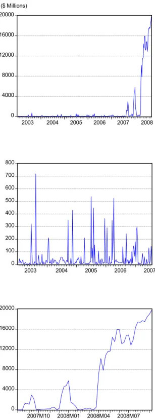
The steps taken by the Federal Reserve to make discount window credit more accessible did lead to an increase in the volume of discount window borrowing, as shown in Figure 1. The upper panel in the figure shows total outstanding primary credit since the establishment of the facility in 2003. Due to the enormous increase in borrowing during the crisis period, the middle and the lower panels split the sample period in August 2007 to make the earlier period more visible.
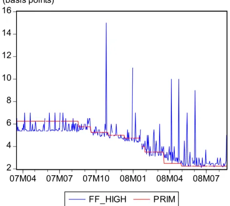
While the massive increase in the volume of borrowing supports the argument that the stigma of borrowing has been eliminated, one should be cautious in not declaring a victory too quickly. Figure 2 shows the highest traded funds rate against the primary credit rate. It reflects that despite the enormous increase in the volume of borrowing, some trades in the funds market took place at rates above the primary credit rate on occasion. What is comforting about these findings, however, is that they are consistent with the predictions of our earlier work. As indicated in Artuç and Demiralp (2008), the reluctance to borrow from the Federal Reserve has several components. The non-price mechanism that is described earlier is the component that is attributable to the Federal Reserve officials’ implementation of discount lending. Artuç and Demiralp (2008) showed that this component has declined significantly after the establishment of the new facility in 2003. Meanwhile, a second type of stigma arises from the asymmetric information problems associated with discount window borrowing. Specifically, while most banks borrow from the discount window, sometimes the facility is also used by troubled or failing institutions. Because market participants cannot fully differentiate healthy from troubled
borrowers, they may view borrowing as a potential sign of weakness for any bank that visits the window. If this type of stigma increases at the early stages of a financial crisis while the institutions are trying to signal that they are in good shape, it could
explain the spikes in the funds rate over the primary credit rate as seen in Figure 1.1 In
addition, it is plausible to think that the capital crunch during the financial crisis may leave some institutions without sufficient collateral to apply for a primary credit loan and hence these institutions may bid for higher rates in the federal funds market, which is unsecuritized.
The Model
The model that we describe in this section closely resembles the one developed in Artuç and Demiralp (2008), which can be viewed as an extension of the model proposed by Clouse and Dow (1999). Hence, the discussion in the following
paragraphs relies heavily on section three in Artuç and Demiralp (2008). We consider
a framework where bank i’s goal is to keep its daily reserves holdings at a level L1.
Daily reserve balances vary over the course of the maintenance period (see Carpenter and Demiralp, 2006). However, from the borrowing viewpoint, a bank’s decision to borrow from the Fed is a static decision based on the liquidity conditions on each day. Therefore, we do not differentiate across the days of the maintenance period except for the settlement Wednesday which may necessitate higher borrowing because banks have less flexibility in absorbing any reserve shortages on the last day of the
1
Indeed, when we take a closer look at the days with spikes in the funds rate, we observe that market commentaries are consistent with elevated asymmetric information problems. An extreme example is October 25, 2007 when the highest traded funds rate exceeded the primary credit rate by almost ten percentage points. On this day, Wrightson ICAP reported that “the stigma of discount window borrowing was heightened by the news that the New York Fed had extended $400 million of secondary-credit loans on Wednesday. If word got out that a given institution had tapped the window on Thursday, the market might speculate that the bank in question was the same one that had been forced to make use of the higher-cost secondary credit program for shaky institutions the day before. The reputational damage of a leak of that nature would be disastrous.” (Wrightson ICAP, Fed Funds Monitor, www.wrightson.com)
maintenance period. On this day, the desired level of reserve holdings are determined by L2.
Banks’ balance holdings follow a stochastic process. During the day, there are
aggregate and individual shocks to the average level of reserve balances (
_
R), which
sets the balance of bank i equal to:
Rti =R+Ut +Vti
_ (1)
where Ut ~N[0,XU] is an aggregate shock2 and i ~ [ V, V]
t U X X
V − is an
individual shock where XU is the standard deviation of the aggregate shock while
V
X represents the support of the mean zero uniform distribution. Hence, the
individual bank becomes a lender in the funds market if Ri L
t > and demands funds if
L
Rti < for L=L1,L2
Banks that are short of reserves have two options: they either choose to borrow from the funds market or they borrow from the Federal Reserve. If the bank
chooses to borrow φt dollars from the funds market, the cost per dollar is the market
interest rate rt. Alternatively, if the bank borrows φt dollars from the Federal
Reserve, the cost per dollar is the discount rate (or the primary credit rate after 2003),
f
r , plus a fixed cost c. Thus, total cost per dollar is
t f
c r
φ
+ . Because of the fixed
cost, partial borrowing from the Federal Reserve is not optimal and a bank either
prefers to borrow entirely from the Federal Reserve or from the funds market.3
2
Because the original model is estimated by removing the outliers, we cut 0.5% from the tails of the normal distribution.
3
Without loss of generality, one may think of the fixed costs of borrowing to vary with each bank, reflecting the particular bank’s relative hesitance to borrow from the discount window based on factors such as the size of borrowing, the history of borrowing, or the availability of credit lines in the funds market. While we model it in a homogenous manner for simplicity, modeling it in a heterogenous manner is also trivial and it does not change any of the implications of our model.
In addition to borrowings from the Federal Reserve that are driven by market conditions, there are also borrowings due to technical difficulties such as network problems which force banks to borrow from the Fed regardless of market conditions.
In order to capture this type of borrowing, we assume that a random fraction, pt, of
the banks will face a technical problem in the system where pt has a uniform
distribution: pt ~ U[0, F].
We assume that there is a continuum of banks, indexed from 0 to 1. Thus there are an infinite number of banks with zero individual measure whose measure integrates to 1. Indexing is done according to reserve balance levels such that a bank with the lowest level of reserve balances is indexed to 0 and the one with the highest level of reserve balances is indexed to 1. .
Total demand for funds has two components. It can be met in the funds market or it can be met at the discount window. The equilibrium federal funds rate,
t
r, is determined by the market equilibrium when the total supply of funds is equal to
the total demand for funds. In modeling the borrowing behavior, our focus is on individual trades in the funds market and on days of market tightness because these are the days on which borrowing from the Fed are more likely. Therefore, we set the daily high funds rate equal to:
t t high
t r
r = +ω where ωt ~(0,s) (2)
Equation (2) notes that the maximum funds rate that is registered for a given day will differ from the equilibrium funds rate depending on the reserve need and the bargaining power faced by the counterparties of that particular trade, represented byωt.
Turning to the days without tightness, on these days trades are almost always cleared in the funds market unless there is a technical problem. For that reason and without loss of generality, if supply is larger than demand, we simply set the funds
rate (rt) equal to the marginal benefit of holding balances as in Clouse and Dow
(1999). Hence, a bank can offer reserves in the funds market if the market rate is greater than the marginal benefit of holding balances.
If the fixed costs of borrowing decline in the period after 2003, then,
everything else remaining the same, this implies a decline in the volatility of the funds rate in the post-2003 period and an increase in the sensitivity of discount window borrowing to the funds rate (a more detailed discussion about the implications of the model can be found in Artuç and Demiralp, 2008). This implied change in volatility and the revival of the borrowing function allows us to identify the size of the implicit cost before and after 2003.
If we could attribute the entire decline in fed funds volatility to the new discount facility, we could proceed with estimation without any second thoughts. However, the decline in fed funds volatility is also influenced by certain other
developments such as better liquidity management by the Trading Desk (see Demiralp and Farley, 2004), improvements in internal information systems (including those that track the balance in a bank’s Federal Reserve account), or banking industry
consolidation. In order to minimize the effects of such factors on fed funds volatility, we keep our sample period relatively recent, and start it in 1998. Furthermore, to
control for any remaining effects of such factors, we allow the distributions of Ut and
i t
V to get wider or narrower in a linear fashion over time. That is we let:
t D A
XU = + × and XV =B+E×t (3)
To identify the potential decrease in the stigma associated with discount window borrowing, we consider the following specification for the implicit borrowing cost c: 1 c c = , prior to 2003 2 1 c c c = + , after 2003
Note that the above specification treats the implicit costs of borrowing to be exogenously determined. An alternative and a more plausible strategy would be to model the costs of borrowing as a function of the amount borrowed from the Federal Reserve. However, modeling the cost of borrowing endogenously cannot be
identified in our set up and we leave this issue as a topic for future research.4
In order to estimate our model, we use “Indirect Inference”. Indirect Inference uses the estimates of an auxiliary model (rather than moments) to compare the actual and the simulated data. Because we can think of the moments of the data as the parameters of a simplified auxiliary model, Method of Simulated Moments (or GMM) can be considered as special cases of Indirect Inference. An auxiliary model does not need to be “correct” for Indirect Inference to give consistent results. So long as the selected auxiliary model summarizes the data well, the estimates of the actual model will be consistent and asymptotically normal. This is because the auxiliary model is only used to extract information about the underlying data generating process and provided that the parameter estimates from the actual data are close to those from the simulated data, whether both of these estimates are biased or not is of secondary importance. In other words, the auxiliary parameter estimates themselves do not carry much meaning other than being indicators of how closely the simulations match the
4
data (see Artuc and Demiralp, 2008. For a more technical reading on Indirect Inference, see Gourieroux, Monfort, and Renault, 1993; Smith, 1993).
We contemplate a simple borrowing function as the auxiliary model. The auxiliary borrowing function summarizes how borrowing from the Fed changed over time and after the policy change in 2003 through a simple OLS regression, shown in equation (4). In addition to the OLS estimates, we use the mean and the variances of borrowing and the spread between the daily high funds rate and the target as part of the auxiliary model (equations (5) through (8)). We also add the lowest 50 percent of the spread between the daily high funds rate and the target to capture the volatility in the funds rate in the absence of market tightness (equations (9) and (10)). The estimation strategy is to find the parameters that will make the simulations of the model and the actual data look as similar as possible with respect to the auxiliary model’s OLS estimates and moments. Specifically, our auxiliary model is:
t Wed Settl t t t t r t tr D r D BR =β +β +β +β +β +β6 . .+ε ~ 2003 5 ~ 4 3 ~ 2 1 (4) t t BR =β7 +ε2 (5) t t r 8 3 ~ ε β + = (6) t t BR 7)2 9 4 ( −β =β +ε (7) t t r 8 2 10 5 ~ ) ( −β =β +ε (8) t t r 11 6 ~ 2 =β +ε (9) t t r2 11 2 12 7 ~ ) ( −β =β +ε (10) and
[
]
, 12 2 1 β ... β β β =where BRt is the amount of borrowing from the Fed normalized by required operating
balances, rt
~
is the spread between the funds rate and the funds rate target, t is the time
trend, D2003 is a dummy for days after the policy change, DSettl.Wed. is a dummy for
the Settlement Wednesday, εt is an iid random shock, T is the sample size, and r2t
~
is
the lowest 50 percent of rt
~
.
Let
^
β be an OLS estimate of β from the actual data and
~
β be an estimate of
β from the simulated data. We pick the model’s parameters
⎥⎦ ⎤ ⎢⎣ ⎡ 2 __ 2 1c DEF R s L c B A such that ' ~ ^ ~ ^ ⎟ ⎠ ⎞ ⎜ ⎝ ⎛ − ⎟ ⎠ ⎞ ⎜ ⎝
⎛ −β β W β β is minimized, where W is the
weighting matrix that is equal to the inverse of the covariance matrix of β.
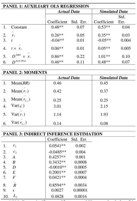
In estimating the model, we exclude those days when the daily high funds rate exceeds the target rate by more than 25 percent to obtain a more realistic distribution for the shocks in the model. Our estimation results (shown in the appendix) suggest that the implicit fixed cost of borrowing declines about 90 percent (from 0.054 to 0.007) after the policy change in 2003. This is strong evidence that the Fed’s new policy was indeed successful in reducing the stigma associated with discount window borrowing.
Simulation Analysis
In this section, we use our model to analyze the role of the Federal Reserve’s primary credit lending facility in calming money markets in the face of the liquidity crisis. Specifically, we ask the following questions:
1) What are the effects of the establishment of the new lending facility on total borrowing and interest rates? In particular, what would the crisis picture look like if the implicit costs of borrowing had not been reduced with the new regime in 2003?
2) What are the implications of increased term of discount lending in
the funds market?
3) What are the effects of the narrowing of the spread between the
primary credit rate and the target rate in calming the money market?
4) What will be the implications of interest payment on reserves for
discount window borrowing?
We first remind that the model described in the previous section is designed to capture the “normal times” of healthy functioning markets. Our estimation period captures a period of a relatively stable structural environment. The sample period starts on June 30, 1998 with the switch from contemporaneous reserves accounting to lagged reserves accounting. It ends on March 19, 2007, a few months prior to the first outbreak of the liquidity crisis in August 2007. Indeed, if we use the estimates from our model for out-of-sample simulations, the severity of the crisis and the model’s inability to forecast this environment becomes clear. Figures 3 and 4 compare the actual data with the model’s out-of-sample simulations for the deviation of the daily high funds rate from the target and for the outstanding primary credit respectively. While our model is a daily model, we present the results in terms of monthly averages to provide visual clarity. The vertical line corresponds to the end of our estimation period in March 2007. There is a wide discrepancy between the data and the model’s simulations, indicating that the period after August 2007 represents quite
extraordinary circumstances which cannot be captured by the estimates prior to August 2007, as we would expect.
The sizable discrepancy between the data and the simulations for the crisis period suggests that we should first incorporate the crisis circumstances into our model before we can conduct any counterfactual experiments about the efficiency of the Federal Reserve’s policies. At this point, we make several assumptions to
replicate the conditions during the crisis. In order to capture the overall need for short
term liquidity, we increase the volatility of the aggregate shock Ut. Furthermore, the
increase in the term of the borrowing is expected to reduce the implicit costs of
borrowing by making it more convenient to lengthen the duration of a loan.5
In order to match the moments of the data, we double the standard error of the
aggregate shock Utand reduce the costs of borrowing by one half, which allows us to
obtain more reasonable estimates for the interest rate spread and the volume of borrowing during the crisis period (Figures 5 and 6). We call these simulations the “benchmark simulations”. In evaluating the performance of the model, one should be careful not to be tempted to use the eyeball metric to compare the simulated series against the actual data because this gives the wrong impression that the model’s job is to match the actual data on a day-by-day basis. Instead, our goal is to match the underlying data generating process, and the estimation results in Table A1 reflect that the model does reasonably well in achieving this goal. Indeed, even if we match the underlying data generating process perfectly, the simulated series will differ from the actual data due to the presence of random shocks.
5
The Federal Reserve may have also reduced the implicit costs of discount borrowing indirectly by introducing several other lending facilities and making the overall borrowing from the Fed more accessible.
We now proceed and analyze the questions that were raised at the beginning of this section. The first question that we tackle is the effects of the policy change in 2003 in mitigating the crisis after 2007. In other words, had the Fed not changed its lending policy in 2003, what would the picture look like in the funds market? Based on our findings in Artuç and Demiralp (2008), we would expect the volatility in the funds market to worsen significantly in the absence of the new regime because the current practice allows the needy institutions to utilize this service without much hesitation. Figure 7 confirms our expectations. In this figure, we plot the actual spread between the daily high funds rate and the target (the dotted line) as well as the simulations that are generated by our benchmark model (the dashed line). In addition, we show the spread under the counterfactual experiment where the cost of borrowing remained at its pre-2003 level (the bold line). As can be seen, the counterfactual series skyrockets during the crisis period suggesting that the Federal Reserve’s switch to the new lending regime was very effective in containing the severity of the crisis in the money market.
Turning from prices to quantities, the volume of borrowing cannot be different between the two regimes because banks need to borrow the necessary amount of reserve balances to avoid an overdraft or a reserve deficiency in our model. For this reason, in reporting our simulation results we only present the spread between the daily high funds rate and the target rate and do not show the borrowing behavior when the latter is unaffected under different scenarios.
Next, we analyze the effectiveness of the changes in the primary credit facility that the Federal Reserve has introduced since the beginning of the crisis. Recall that our benchmark model implied a 50 percent decline in borrowing costs during the crisis period. In assessing the implications of extended terms of borrowing, we keep
the fixed cost of borrowing at its pre-crisis level and simulate the interest rate spread under this scenario. Figure 8 displays the results from this exercise. The elevated volatility under the counterfactual scenario indicates that extending the term of the borrowing was an effective action in reducing the implicit costs of borrowing and hence controlling the volatility in the funds market.
While the term of the borrowing was extended, the Federal Reserve also narrowed the spread between the primary credit rate and the target rate from 100 basis points to 25 basis points over the course of the crisis. Our earlier findings in Artuç and Demiralp (2008) would suggest that the primary credit rate works as an upper bound in the absence of market stigma and that a decline in this rate should decrease deviations of the funds rate from the target. Our next simulation keeps the spread between the primary credit rate and the target unchanged at 100 basis points. As shown in Figure 9, the counterfactual spread is at least as high as the benchmark simulation, if not higher. This elevated volatility suggests that narrowing the spread was effective, even though the difference between the counterfactual and benchmark simulations is not as outstanding as in the previous experiments probably due to the increased need for collateral under the crisis circumstances. That is, because federal funds borrowing is unsecuritized whereas discount window borrowing requires collateral, certain banks may still need to borrow in the funds market by paying a higher premium if they do not have the sufficient collateral for discount borrowing.
Recently, the Federal Reserve has been granted the authority to pay interest on reserve balances. In addition to placing a theoretical lower bound on the funds rate, interest payments on reserve balances may increase the demand for balances simply because the cost of holding these balances are now lower. Our last exercise considers the impact of a higher level of balances in controlling the funds rate volatility. While
it is hard to guess the precise magnitude of the change in reserve balances, we increase the average normalized reserve balances by 10 percent in our counterfactual experiment. Figure 10 shows that the control over interest rates improve while Figure 11 shows that the need for borrowing declines if the average balance holdings
increase as predicted under this new regime. Together, these results suggest that any policy change that causes an increase in reserve holdings, such as interest payment on reserves, is quite helpful in controlling money markets.
Conclusions
In this paper, we analyzed the effectiveness of various changes adopted by the Federal Reserve since the outbreak of the liquidity crisis in August 2007. We showed that the steps taken to reduce the implicit costs of borrowing were more effective in calming the money market while narrowing of the spread between the primary credit rate and the target was not as effective. Would the Federal Reserve be well-served to keep these changes to its borrowing facility indefinitely? Our results suggest that the spread between the primary credit rate and the target rate can be increased back to 100 basis points without much impact on financial markets. Meanwhile, the recent policy change of interest payment on reserves should make it easier for the Desk to maintain the target permanently, not only by placing a lower bound for the funds rate but also by increasing the level of reserve balances, which should reduce the demand for borrowing and ease the consequent tightness in the funds market.
References:
Artuç, Erhan and Selva Demiralp. (2008). “Discount Window Borrowing after 2003: The Explicit Reduction in Implicit Costs.” Koc University ERF Working paper: 0708
Carpenter, Seth and Selva Demiralp. (2006). “The Liquidity Effect at a Daily
Frequency.” Journal of Money, Credit, and Banking,38 (June), 901-920
Clouse, James.A. and James.P. Dow. (1999). “Fixed Costs and the Behavior of the Federal Funds Rate.” Journal of Banking and Finance, 23, 1015-1029
Darrat, Ali F., Khaled Elkhal, Gaurango Banarjee, and Maosen Zhong. (2004). “Why do US Banks Borrow from the Fed? A Fresh Look at the ‘Reluctance’ Phenomenon.” Applied Financial Economics, 14, 477-484
Demiralp, Selva and Dennis Farley. (2005). “Declining Required Reserves, Funds Rate Volatility, and Open Market Operations.” Journal of Banking and Finance, 29, 1131-1152.
Dow, James P. (2001). “The Recent Behavior of Adjustment Credit at the Discount Window.” Journal of Macroeconomics, 23, 199-211
Dutkowsky, Don H. (1993). “Dynamic Implicit Cost and Discount Window Borrowing: An empirical investigation.” Journal of Monetary Economics, 32,105-120
Furfine, Craig H. (2001). “The Reluctance to Borrow from the Fed.” Economic Letters, 72, 209-213
Furfine, Craig H. (2003). “Standing Facilities and Interbank Borrowing: Evidence from the Federal Reserve’s New Discount Window.” International Finance, 6 (3), 329-347
Goodfriend, Marvin. (1983). “Discount Window Borrowing, Monetary Policy, and the post-October 6, 1979 Federal Reserve Operating Porcedure.” Journal of Monetary Economics, 12, 343-356
Gourieroux, C., Monfort, Alain, and E. Renault. (1993). “Indirect Inference.” Journal of Applied Econometrics, 8, 85-118
Madigan, Brian and William Nelson. (2002). “Proposed Revision to the Federal Reserve’s Discount Window Lending Programs.” Federal Reserve Bulletin, July, 313-319
Pearce, Douglas K.. (1983). “Discount Window Borrowing and Federal Reserve Operating Regimes.” Economic Inquiry, 31, 564-579
Peristiani, Stavros. (1998). “The Growing Reluctance to Borrow at the Discount Window: An Empirical Investigation.” The Review of Economics and Statistics, 611-620
Smith, Anthony. (1993). “Estimating Nonlinear Time Series Models Using Simulated Vector Autoregressions.” Journal of Applied Econometrics, 8, 63-84
Figure 1: Primary Credit Outstanding (Weekly Average)
0 4000 8000 12000 16000 20000 2003 2004 2005 2006 2007 2008 0 100 200 300 400 500 600 700 800 2003 2004 2005 2006 2007 0 4000 8000 12000 16000 20000 2007M10 2008M01 2008M04 2008M07 ($ Millions)Figure 2: Daily High Funds Rate and the Primary Credit Rate
2 4 6 8 10 12 14 16 07M04 07M07 07M10 08M01 08M04 08M07 FF_HIGH PRIM (basis points)where FF_HIGH: Daily high funds rate
PRIM: Primary Credit rate
Appendix
The first two panels of Table A1 present the OLS estimates of the auxiliary model parameters using the actual as well as the simulated data along with the mean and the
variance of borrowing and rt
~
. Comparing the second and the fourth columns in the first panel, we note that the auxiliary model’s estimates from the simulated data and the actual data are pretty close to each other since the algorithm minimizes the distance between those two estimates. However, they are not identical since the auxiliary model has more parameters than the true underlying model. As shown in
the fifth row, borrowing responsiveness to the interest rate spread (rt
~
) increases significantly after the policy change in 2003 consistent with a decline in the market stigma and the revival of the borrowing function. The second panel provides a similar comparison between the moments generated by the actual data (column 2) and those computed from the simulated data (column 3). Similar to the first panel, the two sets of statistics display a strong resemblance.
The third panel of Table A1 exhibits the parameter estimates of the true underlying model and their standard errors. The most interesting parameters for our purposes are displayed in the first two rows. Notice that the implicit fixed cost of
borrowing declines about 90 percent (from c1 =0.054 to c1+c2 =0.007) after the
policy change in 2003. This is strong evidence that the Fed’s new policy was indeed successful in reducing the stigma associated with discount window borrowing. In addition to estimating the fixed cost of borrowing from the discount window, we are also interested in determining whether this implicit cost exhibits any gradual changes over time. In particular, one may expect a gradual decline in the implicit cost of borrowing in the post-2003 period, due to the market’s slow adjustment to the new regime. In order to address this issue, we experimented with an alternative model
which allows a time trend in the implicit cost of borrowing prior to and after 2003 (not shown). However, the trend terms associated with the implicit cost of borrowing were not significant in either sample. This finding suggests that there may not be a gradual adjustment to the new regime in the second sample. Our results may also be driven by the fact that we may not have a sufficient number of observations to identify such a time trend.
The third row shows that the aggregate reserve shock Ut ranges between -0.43
and +0.43 in the beginning of the sample, while the bank specific reserve shock Vti
varies between -0.34 and 0.34 initially (row 4). Rows 5 and 6 show that there is a
significant time trend in these shocks. In fact, when we substitute the estimates for D
and E in equation 3, we observe that the aggregate reserve shock exhibits a negative
trend while the bank specific shock exhibits a positive trend. The estimate of E
implies that the standard error of Ut decreases about 0.05 percent per year while the
estimate of D implies that the range of Vti increases about 15 percent every year.The
mild negative time trend in the aggregate shock, Ut, could reflect improvements in
the Desk’s reserve management ability over time as we noted in the main text. Row 7 exhibits that the estimated ratio of banks that incur a technical problem, and thus are forced to borrow from Fed rather than the market, vary from 0 to 0.04, indicating that not more than 4 percent of the banks are affected by this type of a problem at a given point in time. The last row indicates that banks aim to attain a higher level of balances on the last day of the maintenance period, consistent with our expectations.
Table A1: Indirect Inference and Auxiliary Model Estimations
PANEL 1: AUXILIARY OLS REGRESSION
Actual Data Simulated Data
Coefficient Std. Err. Coefficient
Std. Err. 1. Constant 0.48** 0.07 0.53** 0.04 2. rt ~ 0.26** 0.05 0.35** 0.03 3. t -0.04** 0.01 -0.05** 0.004 4. t × rt ~ 0.06** 0.01 0.05** 0.005 5. D2003 × rt ~ 0.86** 0.22 1.01** 0.10 6. Settl.Wed. D 0.46** 0.11 0.48** 0.07 PANEL 2: MOMENTS
Actual Data Simulated Data
1. Mean(BR) 0.46 0.45 2. Mean(rt ~ ) 0.42 0.37 3. Mean(r t ~ 2 ) 0.25 0.25 4. Var(ς) 3.01 2.15 5. Var(rt ~ ) 1.14 1.93 6. Var(r t ~ 2 ) 0.14 0.08
PANEL 3: INDIRECT INFERENCE ESTIMATION
Coefficient Std. Err. 1. c1 0.0541** 0.002 2. c2 -0.0485** 0.004 3. A 0.4257** 0.001 4. B 0.3432** 0.0008 5. D -0.0010** 0.0005 6. E 0.2001** 0.0007 7. F 0.0421** 0.0004 8. __ R 0.8594** 0.0034 9. s 0.0027 0.00001 10. L2 0.4828 0.0016
*/** indicates significance at 95 percent and 99 percent level of confidence respectively.
where
BR Normalized borrowing from the Fed
t
r
~ Daily high funds rate minus the target rate
t
r ~ 2
t Time trend
2003
D Dummy variable for the period after January 6, 2003
. .Wed Settl
D Dummy variable for the last day of the maintenance period
1
c Implicit cost prior to 2003
2
c Implicit cost after 2003
A Interval parameter for the aggregate shock
B Interval parameter for the bank specific shock
D Time trend parameter for the aggregate shock
E Time trend parameter for the bank specific shock
F Interval parameter for the probability of a technical problem
__
R Average reserve balances
s Variance of the noise parameter for the daily high funds rate
2