Measuring the driving forces of the owner-occupied and rental housing market - A DSGE analysis

(1)

Measuring the Driving Forces of the

Owner-Occupied and Rental Housing

Markets - A DSGE Analysis

Economics Section, Cardiff Business School

Robert Forster

November 27, 2018

A Thesis Submitted in Fulfillment of the Requirements for the Degree of

Doctor of Philosophy of

Cardiff University

Thesis Supervisors

Dr Vo Phuong Mai Le

Professor Patrick Minford

(2)

27/11/2018

(3)

Abstract

This thesis analyses the developments of the U.S. owner-occupied and rental housing markets. Furthermore, it evaluates whether loose monetary policy fuelled the housing boom and therefore contributed heavily to the latest financial crisis. The dissertation findings originate from two estimated DSGE models which accommodate a combination of various, distinct features. In contrast to the literature, I introduce a banking sector into the model economy and allow for a choice between either renting or owning a home. Accounting for these characteristics enables us to capture frictions arising from the banking sector on the one hand and to properly model the change in the homeownership structure on the other. Based on this framework, the second DSGE model relaxes the assumption of a fixed housing supply and introduces sticky prices into the consumption sector. The contributions of this dissertation are twofold. First, it determines the driving forces behind the pre and post-crisis movements of the rental and owner-occupied housing sectors. The results suggest that the latest rise in rental housing is driven by a combination of various factors, such as default, bank lending, change in preferences and news about the economic outlook. Furthermore, news about future productivity increases had a significant effect on house prices before and after the financial crisis. A robustness check confirms these findings. The second contribution is to show that accommodative pre-crisis monetary policy was not the main cause of the latest housing boom, as argued in one branch of the literature. Instead, bank lending behaviour and fundamentals played a key role in the expansion of the owner-occupied housing market. The dissertation finishes with a macroprudential policy evaluation.

(4)

Acknowledgements

This PhD was funded by the Sir Julian Hodge Bursary of Applied Macroeconomics and the Economic and Social Research Council.

I would like to thank both of my supervisors, Vo Phuong Mai Le and Patrick Minford, for their guid-ance, comments and critical discussions. Thanks also to Wojtek Paczos, David Meenagh, Huw Dixon and Konstantinos Theodoridis who were always available to talk to me about my research.

I am very grateful for the enriching and stimulating conversations with Luis Matos, Timothy Jackson, Gai Yue and the rest of my PhD cohort.

Thanks to my friends Leo, Max, Florian, Michael, Simon, Jörg, Andy and Dario. You helped me to take my mind off economic related problems.

Special thanks to my mother, father and brother who continuously supported me throughout my PhD studies. Without you this would have not been possible.

(5)

List of Figures

1 Rental Housing vs. Owner-occupied Housing; Source: U.S. Census Bureau . . . 2

2 Home Sales and Housing Affordability; Source: Taken from the presentation by Bullard (2012) 4 3 Housing Starts: New Privately Owned Housing; Source: U.S. Census Bureau . . . 5

1.1 Ratio of rental to owner-occupied housing: 1985Q1 - 2010Q4, Source: U.S. Census Bureau . 11 1.2 Data used for estimation . . . 22

1.3 Impulse response to a one standard error household default shock . . . 27

1.4 Impulse response to a one standard error aggregate spending shock . . . 28

1.5 Impulse response to a one standard error housing demand shock . . . 29

1.6 Impulse response to a one standard error household LTV shock . . . 30

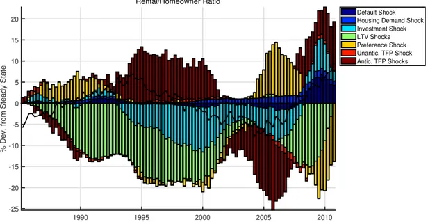
1.7 Shock decomposition of the rental/homeowner ratio, the solid black line depicts the smoothed series. . . 33

1.8 Shock decomposition of real house prices . . . 36

1.9 Shock decomposition of real rental prices . . . 36

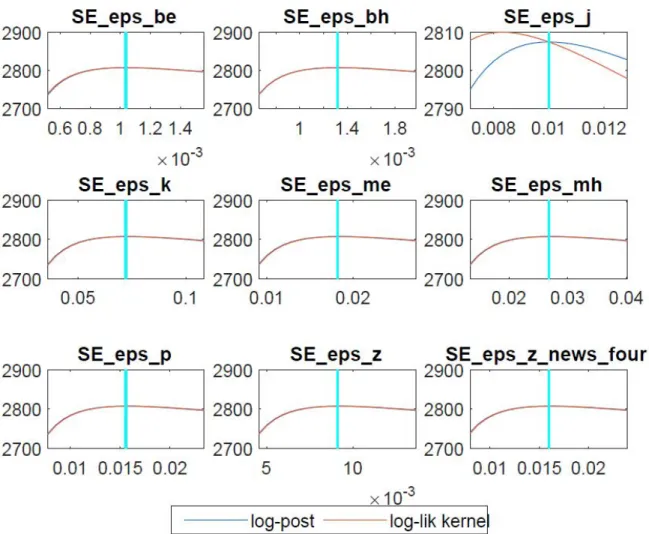
1.10 Mode Plots: Upper panel: σbe,σbh,σj. Middle panel: σk,σM E,σM H. Lower Panel: σp,σ0z,σz4. 55 1.11 Mode Plots: Upper panel: σ8 z,η, ϕDB. Middle panel: ϕDH, ϕKE, ϕKH. Lower Panel: ϕEB, ϕEE,ϕSB. . . 56

1.12 Mode Plots: Upper panel: ϕSS, κS,Ωr. Middle panel: µ,ν,ρD. Lower Panel: ρE,ρS,σ. . . 57

1.13 Mode Plots: Upper panel: θS,ζE, ζH. Middle panel: ρbe,ρbh, ρj. Lower Panel: ρk,ρme,ρmh. 58 1.14 Mode Plots: Upper panel: ρp,ρz. . . 59

1.15 MCMC Convergence: Upper panel: σbe. Middle panel: σbh. Lower Panel: σj. . . 60

1.16 MCMC Convergence: Upper panel: σk. Middle panel: σme. Lower Panel: σmh. . . 61

1.17 MCMC Convergence: Upper panel: σp. Middle panel: σz0. Lower Panel: σz4. . . 62

1.18 MCMC Convergence: Upper panel: σ8 z. Middle panel: η. Lower Panel: ϕDB. . . 63

(9)

1.20 MCMC Convergence: Upper panel: ϕEB. Middle panel: ϕEE. Lower Panel: ϕSB. . . 65

1.21 MCMC Convergence: Upper panel: ϕSS. Middle panel: κS. Lower Panel: Ωr. . . 66

1.22 MCMC Convergence: Upper panel: µ. Middle panel: ν. Lower Panel: ρD. . . 67

1.23 MCMC Convergence: Upper panel: ρE. Middle panel: ρS. Lower Panel: σ. . . 68

1.24 MCMC Convergence: Upper panel: θS. Middle panel: ζE. Lower Panel: ζH. . . 69

1.25 MCMC Convergence: Upper panel: ρbe. Middle panel: ρbh. Lower Panel: ρj. . . 70

1.26 MCMC Convergence: Upper panel: ρk. Middle panel: rhome. Lower Panel: ρmh. . . 71

1.27 MCMC Convergence: Upper panel: ρp. Middle panel: ρz. σj. . . 72

1.28 Trace plot of chain 1, parameterκS. . . 73

1.29 Trace plot of chain 2, parameterκS. . . 74

1.30 Trace plot of chain 1, parameterθS. . . 75

1.31 Trace plot of chain 2, parameterθS. . . 76

1.32 Trace plot of chain 1, parameterΩr. . . 77

1.33 Trace plot of chain 2, parameterΩr. . . 78

2.1 Household Borrowing, Federal Funds Rate . . . 80

2.2 Homeownership Rate . . . 81

2.3 Data used for estimation . . . 93

2.4 Impulse response to a one standard error housing technology shock. . . 98

2.5 Impulse response to a one standard error aggregate spending shock. . . 99

2.6 Monetary Policy Shock, independently and identically distributed. . . 99

2.7 Model comparison based on impulse responses . . . 100

2.8 Shock decomposition of loans to households . . . 103

2.9 Shock decomposition of loans to households . . . 103

2.10 Shock decomposition of house prices based on first-differenced data . . . 104

2.11 Shock decomposition of house prices based one-sided HP filtered data. . . 104

2.12 First-difference filtered data used for the construction of the posterior mode . . . 105

2.13 One-sided HP filtered data used for the construction of the posterior mode . . . 106

2.14 Mode Plots: Upper panel: σbe, σbh, σj. Middle panel: σk, σM E, σM H. Lower Panel: σp, σzc, σzh. . . 121

2.15 Mode Plots: Upper panel: σr,σs,σπ. Middle panel: σN C,σN H,χH. Lower Panel: χS,η,ϕDB.122 2.16 Mode Plots: Upper panel: ϕDH, ϕKE, ϕKC. Middle panel: ϕKH, ϕEB,ϕEE. Lower Panel: ϕSB,ϕSS, ι. . . 123

(10)

2.17 Mode Plots: Upper panel: κS,κN_H,κN_S. Middle panel: Ωr,µc,ψR. Lower Panel: ψπ, ψY,ρD. 124

2.18 Mode Plots: Upper panel: ρE,ρS,σ. Middle panel: θS,Θπ,ζE. Lower Panel: ζH,ρbe,ρbh. . 125

2.19 Mode Plots: Upper panel: ρj,ρk,ρme. Middle panel: ρmh,ρp,ρzc. Lower Panel: ρzc. . . 126

3.1 Average Mortgage LTV ratios: Mortgaged Homeowner vs. All Homeowners, 1970Q1 - 2011Q4; Source: Taken from the presentation by Bullard (2012) . . . 129 3.2 Countercyclical LTV Rule vs. Endogenous Housing Supply . . . 134

(11)

List of Tables

1.1 Calibrated Parameters . . . 23

1.2 Prior and Posterior Distributions, Structural Parameters . . . 24

1.3 Prior and Posterior Distributions, Shock Processes . . . 26

1.4 Conditional and Unconditional Variance Decomposition . . . 31

1.5 Historical Decomposition of the Rental/Homeowner Ratio . . . 34

1.6 Robustness, Shock Processes . . . 38

1.7 Robustness, Posterior Modes without Loan Losses . . . 39

2.1 Calibrated Parameters . . . 92

2.2 Prior and Posterior Distributions, Structural Parameters . . . 94

2.3 Prior and Posterior Distributions, Shock Processes . . . 96

2.4 Theoretical Moments vs. Data . . . 97

2.5 Variance Decomposition . . . 101

2.6 Robustness, Posterior Modes without Loan Losses . . . 107

2.7 Theoretical Moments vs. Data (Excluding Loan Losses) . . . 108

3.1 Welfare Effects of Applying a LTV rule . . . 138

(12)

Introduction

Housing has made it into mainstream economics and is an essential component in modern financial friction models. Recent events have shown that housing market developments are not just the result of various macroeconomic changes, but can also trigger substantial business cycle fluctuations. U.S. housing wealth (i.e. the residential capital stock at market price), is considerably larger than GDP and fluctuates substantially over time. Between 1952 and 2008, the average housing wealth to GDP ratio was 1.5. However, in 2005 this ratio reached a value of 2.26. This year also marks the start of the housing market correction, where growth in housing wealth and the ratio of housing investment to GDP fell dramatically (Iacoviello 2010).

Today we know that housing was at the roots of the latest financial crisis, which has caused severe devastation to the U.S. economy. Pre-crisis developments showed alarming trends for many housing variables that were either misjudged or remained unnoticed by governments and authorities. What followed was a sharp contraction of housing markets accompanied by falling asset prices and a collapse of residential investment. In addition to this, owner-occupied housing experienced a rapid increase in the years leading up to the crisis, whereas rental housing showed a decline. However, this comes to a halt right before the outbreak of the Great Recession. Owner-occupied housing declined from 2009 onwards and rental housing instead increased steeply. Figure 1 illustrates these developments of both housing sectors.

(13)

1987 1990 1992 1995 1997 2000 2002 2005 2007 2010 2012 2015 58 60 62 64 66 68 70 72 74

Units (in Millions)

32 34 36 38 40 42

Units (in Millions)

Howeowner Rental

Figure 1: Rental Housing vs. Owner-occupied Housing; Source: U.S. Census Bureau

The crisis not only effected the credit supply and various other channels of the economy, but also triggered a change in the homeowner status of many households. Based on these facts the objectives of this dissertation are twofold: First, it investigates the driving forces behind both housing markets. Second, the thesis measures to what extent monetary policy has influenced the pre-crisis expansion of household debt and house prices. The underlying methodology is an estimated DSGE model, which accommodates a banking sector and explicitly features a choice between rental and owner-occupied housing. The framework is also equipped with collateral constraints that allow households to borrow against their homes values. As an asset price drop can have severe consequences to the borrowing ability of agents, this mechanism is better known as a financial accelerator. Through the additional constraint, shocks get amplified and intensify the responses of economic agents. It was first developed by Kiyotaki and Moore (1997) and later updated by Iacoviello (2005), who replaced land by housing. There is a second, very popular financial accelerator approach, which is widely used in the literature. Again, this mechanism was introduced long before the financial crisis by Bernanke and Gertler (1989). The origins of this type of financial accelerator framework go back to the costly state verification methodology proposed by Townsend (1979). The state of the borrowers’ balance sheet takes up a crucial role under this mechanism. It shows that the net worth of a borrower/entrepreneur is inversely correlated with the agency costs (e.g. monitoring of a loan) of undertaking physical investments. This triggers an accelerating effect on investments. The net worth of borrowers is likely to be high during good times of the economy and low during bad times. More solvent consumers will cause a rise in demand for investments and amplify the economic boom phase. The opposite will occur during bad times (Bernanke

(14)

and Gertler 1989). The two concepts discussed above are two common ways to introduce financial frictions into our models and the paper by Forlati and Lambertini (2011) has even combined both mechanisms. Since this dissertation focusses specifically on the developments of the U.S. housing market, the collateral constraint framework has been chosen for the models presented in chapter 1 and 2. As it is standard in the literature, housing consumption in the form of housing services enters the utility function of households.1

Houses are a durable good and can be used for two purposes. First, it serves as collateral for borrowers and second, it delivers utility services. In other words, the households’ accumulated housing stock provides them with a flow of housing services. This collateralizable stock of housing can then be used for their borrowing activities. The flow of residential investment shows up in the borrower’s budget constraint in the form ofHt−(1−δ)Ht−1, whereHtrepresents housing services (i.e. the end-of-period housing stock) andδ

the depreciation of the durable good (Monacelli 2009). Furthermore, I assume proportionality between the stream of housing services and the stock of housing.

As we are going to see later, the demand for housing is subject to an exogenous shock. The disturbance enters the utility function of agents and depending on the sign it either triggers a reduction or increase in the demand for homes. This exogenous process is better known as a housing demand shock. Figure 2 delivers evidence why previous studies have implemented this type of shock. Even though it was more expensive to buy a house during the pre-crisis years, home sales increased sharply until the end of 2005. The collapse of the housing market caused a severe contraction of home sales between 2006 and 2008. As affordability2

of homes increased in the years after the crisis home sales did not follow the same trend. Hence, these developments reflect the rise and decline in the demand for homes before and after the housing boom. The preference shock therefore captures shifts in the demand towards housing which can be caused by changing age shares of a country’s total population (Sun and Tsang 2017). Modelling these socio-economic factors in a DSGE setup can be difficult and hence we assume that they are represented by an exogenous process. This dissertation contributes to the literature in two directions. First, it finds that the latest changes in the U.S. home ownership structure were caused by a combination of four factors. These are default, household preferences, bank lending and news about the economic outlook. The results confirm and extend the findings outlined in the report of the Joint Center for Housing Studies (2013). News about the economic outlook

1_{See for example the papers by Davis and Heathcote (2005), Chang (2000), Baxter (1996), Greenwood and Hercowitz (1991)}

or Matsuyama (1990).

2_{The affordability index comes from the National Association of Realtors (NAR). The index shows whether or not a typical}

household is able to qualify for a mortgage in order to buy a typical home. The typical household corresponds to the median income family as defined by the U.S. Bureau of the Census. A typical home is described as the national median-priced, existing single-family home as computed by NAR. The current interest on mortgages is defined as the effective rate on loans coming from the Housing Finance Board. These parameters are used to illustrate if the median income household is able to obtain a mortgage for a median-priced house. For example, if the index takes the value 100 then this means that a household with a median income has exactly enough financial resources available to qualify for a mortgage on a typical home.

(15)

are also an important driving force behind rental and house price fluctuations. This is in line with the study conducted by Lambertini, Mendicino, and Punzi (2017), which confirms that TFP news are able to trigger a boom and bust of the housing market. Second, the results of this dissertation show that monetary policy only played a minor role in the dangerous pre-crisis growth of household debt and house prices. The literature on this topic has produced ambiguous outcomes. For example papers by Eickmeier and Hofmann (2013) and Bordo, Landon-Lane, et al. (2014) conclude that accommodative monetary policy played a key role during the time prior to the crisis. In contrast, studies by Dokko et al. (2011) and Nelson, Pinter, and Theodoridis (2018) illustrate that monetary policy was not the main cause behind pre-crisis developments. The model in this dissertation identifies fundamentals and bank lending as the main contributors behind the swift increase in home prices and household loans in the years leading up to the financial crisis. Regarding the latter, Demyanyk and Van Hemert (2009) and Dell’Ariccia, Igan, and Laeven (2008) show that excessive risk taking by banks rose and lending standards deteriorated sharply.

Figure 2: Home Sales and Housing Affordability; Source: Taken from the presentation by Bullard (2012)

The question remains in what way this dissertation differs from the studies mentioned above. First of all both chapters, 1 and 2, include a rental market and feature a banking sector. In most of the literature the latter is

(16)

usually assumed away and financial frictions can only arise from the household’s side. However, the banking sector played an important role before and after the financial crisis. Therefore, I relax this assumption and allow for banks, which themselves are credit constrained. Furthermore, the dissertation models endogenously the construction of new homes. A construction sector is often non-existent in many DSGE studies due to the assumption of a constant housing supply. However, figure 3 illustrates that construction activity of new homes3_{increased constantly between the early 1990s and 2006. With the contraction of the housing market}

construction activity drops dramatically and reaches a low in 2009.

1985 1987 1990 1992 1995 1997 2000 2002 2005 2007 2010 2012 2015 0.6 0.8 1 1.2 1.4 1.6 1.8 2

Units (in Millions)

Housing Starts

Figure 3: Housing Starts: New Privately Owned Housing; Source: U.S. Census Bureau

The outline of this dissertation is as follows. Chapter 1 develops a DSGE model, which allows for a rental and owner-occupied housing market. Furthermore, it combines traditional financial frictions with disruptions arising from a banking sector. Additionally, news shocks are introduced into the TFP shock structure, following the work of Schmitt-Grohé and Uribe (2012). In chapter 2, I relax the assumption of a constant housing supply and account for price rigidities in the consumption sector. Chapter 3 presents a discussion about policy implications based on the results in chapter 2. Furthermore, it evaluates the welfare implications of such prudential measures. The relevant literature is discussed separately in each of the chapters. Finally, the dissertation finishes with concluding remarks. However, before we arrive at the main body of the thesis, the next section discusses briefly the estimation strategy used in this dissertation.

3_{The U.S. Census Bureau refers to housing starts as the construction of new housing, where the “}_{start of construction occurs}

(17)

Bayesian Estimation

A popular approach in applied work is the use of Bayesian techniques to determine the underlying model coefficients. One advantage of this estimation procedure is the incorporation of prior information about the parameters in question. Therefore, this section briefly outlines the estimation procedure applied to the models presented in this thesis. The heart of Bayesian econometrics is Bayes’ theorem. Consider two random variables denoted byC andD. The joint probability ofC andDoccurring at the same time can be defined as:

p(C, D) =p(C|D)p(D), (1)

wherep(C, D)stands for the probability ofC andDoccurring, p(C|D)is the conditional probability ofC

occurring depending onD having occurred and p(D) is the marginal probability of D. Alternatively, the joint probability ofC andD could have been defined as:

p(C, D) =p(D|C)p(C). (2)

This allows us to solve forp(D|C)by equating both expressions, which yields the following key result:

p(D|C) = p(C|D)p(D)

p(C) . (3)

We have derived Bayes’ rule. However, in practice things are slightly more complicated. The majority of economic models consists of many different coefficients and when taken to the data, various observables have been chosen for the estimation. Let nowy be a matrix or vector of data andB a matrix or vector of parameters which aims to explainy. Based on the datay, we are interested in finding out about the values inB. Applying Bayes’ rule and replacingD byBandC byy we end up with:

p(B |y) =p(y| B)p(B)

(18)

For us p(B |y)is the expression of fundamental interest. It answers the question what our knowledge ofB

is, given the underlying data. As we are only concerned about the parameters described byB, we can ignore the denominatorp(y)since it does not involveB. This leaves us with the result:

p(B |y)∝p(y| B)p(B). (5)

The left hand side p(B |y)is better known as the posterior density. The first term on the right hand side

p(y| B)is referred to as the likelihood function andp(B)stands for the prior density. The above relationship therefore states that the posterior density is proportional to the likelihood times the prior. It is also often called the posterior kernel. In other words, the posteriorp(B |y)combines the information contained in the data with our prior view. We can also treat equation 5 as an updating rule, where our prior beliefs are updated after having seen the data (Koop 2003).

The prior densityp(B), is not related to the data and therefore consists of any non-data information describing the parameter vectorB. Put differently, it summarises our knowledge about Bbefore seeing the data. For better illustration assume that B is a parameter which represents returns to scale in the production of output. Usually it is a reasonable assumption that returns to scale are more or less constant. Thus, before we consult the data we have prior knowledge about B and we would expect it to be roughly one. For this reason, the prior information is considered a controversial aspect of Bayesian techniques, as it is subjective. The likelihood function, p(y| B), describes the density of the data conditional on the model’s parameters. It is also known as the data generating process. For example, in the linear regression model it is often assumed that the disturbances follow a Normal distribution. This in turn implies thatp(y| B) is described by a Normal density. Furthermore, a central part of Bayesian thinking is to accept that unknown things such as parameters, models and future data are random variables. It allows us to apply simple probabilistic rules and to conduct statistical inference (Koop 2003).

Applying Bayesian techniques to macro models has three central advantages. First, as pointed out by Fernández-Villaverde and Rubio-Ramírez (2004), Bayesian methods exhibit strong small sample properties. This is particularly important for real life applications. The Bayesian approach yields a very strong per-formance when used to estimate dynamic general equilibrium frameworks. Second, pre-sample information is in most cases extremely rich and very useful. Thus, it would be wrong not to take into account such valuable information and omit it from the analysis. For example, microeconometric evidence can help us to construct our priors. If there is a large set of studies which have estimated the discount factor of individuals between 0.9 and 0.99 then any sensible prior should reflect this information (Fernández-Villaverde 2010).

(19)

Third, Bayesian methods allow us to compare different models based on their log marginal data density. The model with the highest log marginal density (i.e. the most likely model) is preferred over the other models with a lower density. The marginal density summarises the likelihood of the data conditional on the model (Koop 2003, An and Schorfheide 2007).

Having reviewed the fundamental theorem of Bayesian econometrics, we can now move on to the estimation strategy, following An and Schorfheide (2007). The models in this thesis are solved with the help of a first order perturbation approximation. We then can apply the Kalman filter to the resulting linear state space system. This allows us to construct the likelihood function of the underlying model. The next step involves finding the mode(s) of the posterior distribution, which is obtained by maximising the posterior kernel with respect to each parameter. The posterior distribution is simulated around the computed mode using the Random Walk Metropolis-Hastings (RWMH) algorithm. The RWMH procedure is useful in cases where we cannot find a good approximation density for the posterior (Koop 2003).

More technically, the detailed steps are:

1. Maximise the log posterior kernellogp(y| B) + log p(B), with respect to every parameter inB, in order to find the posterior modeB∗_{. This is done by using a numerical optimisation algorithm.}

2. ObtainΠe, which is the inverse of the Hessian at the posterior modeB∗_.

3. Define a starting value by taking a draw B(0) _{from the proposal distribution} _N₍_B∗_{, c}2

0Π)e or directly set a specific starting value.

4. Fors= 1, ..., nsim, draw∆from the proposal distributionN(B(s−1)_{, c}2_Π)e _{. The total number of} itera-tions is given bynsim. A jump fromB(s−1)_{is accepted (}_B(s)_{= ∆}_{) with probability}_min_{₁_{, r}₍_B(s−1)_,_∆_|_y₎_} and rejected (B(s)₌_B(s₋1)_{) otherwise. Let the acceptance probability be}

r(B(s−1),∆|y) = p(y|∆)p(∆) p(y|B(s−1)₎_p₍B(s−1)₎ =

P osterior(∆)

P osterior(B(s−1)₎. (6) Note that the scale factor c2 _{effects the acceptance rate and should be adjusted in such a way that the} Markov chain explores the entire domain of the posterior distribution. This is crucial, as otherwise the chain gets stuck in tale or other regions of the posterior density. For example if the acceptance rate is too small, then the vast majority of candidate draws ∆ are always rejected.4 _{This implies that the chain doest not}

move sufficiently and we need a huge number ofnsim for the chain to explore the entire posterior density. On

4_{A high and low acceptance rate is also reflected by a large and small covariance matrix, respectively. Hence, adjusting the}

(20)

the other hand, a high acceptance probability indicates that∆andB(s₋1)_{will tend to be very close to each} other. As before, in order for the chain to cover the entire posterior density, we require an extremely large value for nsim (Koop 2003). Having successfully constructed the posterior distribution with the algorithm

above, we then choose the posterior mean as the point estimate of the parameter.

It is important to highlight that the above algorithm relies on the inverse of the Hessian, which is often the most efficient way to estimate a model. However, Chib and Greenberg (1995) have shown that asymptotically the Monte Carlo Markov Chain explores the entire posterior parameter space from any point. In fact we only require a positive definite proposal density, which makes the use of the inverse Hessian redundant. However, as this is an asymptotic property, we would require a higher number of draws in order to construct the ergodic distribution. Therefore, working with the inverse Hessian is preferred to alternative procedures. As we are going to see later, the chosen prior distributions of the parameters in question are in line with the existing literature. This avoids arbitrarily picking the parameter priors. Bayesian estimation allows for prior beliefs about the model coefficients, which is different to the maximum likelihood approach. The latter focusses just on maximising the likelihood (i.e. p(y|B)) and therefore it is not necessary to introduce prior beliefs. As Koop (2003) describes it, Bayesian estimation can be treated as an updating process, where prior knowledge is injected and then updated by the data. Thus, the resulting posterior distribution contains data and non-data information. Given the prior distributions and the underlying data, the frameworks presented in this thesis can be considered as the most likely DSGE models.5 _{Having reviewed the estimation approach}

used in this analysis, we can now progress to the first chapter of the dissertation.

5_{Note, a comparison between both models, based on the log marginal densities, would be invalid due to different datasets and}

(21)

Chapter 1

What Explains the Latest Increase in

the U.S. Rental Housing Sector?

Evidence from an Estimated DSGE

Model

(22)

1.1 Introduction

The 2007 financial crisis has not only left many banks and businesses struggling but also triggered a change in the U.S. homeowner structure. Looking at recent housing inventory data, it is evident that there has been a shift away from owner-occupied towards rental housing. Figure 1.1 depicts the rental housing stock relative to the owner-occupied housing stock. The series is log transformed and quadratically detrended. The ratio consistently increased between 1985 and the mid 1990s. Due to the efforts of the United States Department of Housing and Urban Development, owner-occupied housing rises and causes the ratio to fall. However, with the start of the financial crisis the ratio kept increasing and reached a new high in 2010. This development is due to a rise in the rental housing inventory and a decrease in owner-occupied housing.6

1985 1987 1990 1992 1995 1997 2000 2002 2005 2007 2010 -6 -4 -2 0 2 4 6 8

% Dev. from Trend

Rental/Homeowner Ratio

Figure 1.1: Ratio of rental to owner-occupied housing: 1985Q1 - 2010Q4, Source: U.S. Census Bureau

Recent research by the Joint Center for Housing Studies (2013) confirms that there has been an increase in the demand for rental property over owner-occupied housing. Not surprisingly the study identifies the Great Recession as one of the key driving forces behind the latest expansion of the rental market. Loan defaults and home foreclosures have changed the status of many households from homeowners to renters. This triggered an increase in the rental housing stock, as former owner-occupied properties became rental homes. Additionally to insolvency, households experienced further risks of home ownership during the crisis. One example is the inflicted wealth loss due to decreasing home values. Furthermore, news about the economic outlook before and after the crisis could have also influenced households’ decisions to either buy a new home or stay in a rental property. The most important contribution of this chapter is the analysis of how banking

(23)

frictions, loan defaults and productivity news have affected the rental and owner-occupied housing markets. So far studies have ignored these crucial factors when it comes to studying the dynamics of both housing sectors. Therefore, this chapter develops a comprehensive DSGE framework to shed new light on this topic. As I take the model to the data, I use a modified version of the extended Iacoviello (2015) framework which features loan defaults of households and a rich set of frictions. The environment is inhabited by three economic agents: a heterogeneous household, who is divided into a saver and a borrower, bankers and entrepreneurs. In this model banks take up an intermediary role and act as a valve for the flow of resources between lenders and borrowers. More specifically, banks provide household borrowers and entrepreneurs with loans and collect deposits from savers. In addition to this, banks are exposed to loan defaults which arise from the supply and demand side. Hence, allowing for banks to exist introduces a new channel into the model and combines financial and banking frictions. As Iacoviello (2015) shows,7 _{the existence of a}

banking sector has an amplifying impact on house prices which is therefore of particular importance for this study. The second reason why banks are in the model, is based on the results of a Bayesian model comparison conducted by Iacoviello (2015). It shows that the model with a banking sector is preferred to the one without.8 _{Finally, as the financial crisis showed, banks played an important role in the latest boom}

and bust of the U.S. economy.

I assume that only savers accumulate rental housing and earn income by letting it to borrowers.9 _{This in turn}

means that borrowers have to choose between either owner-occupied or rental housing. Hence, it is assumed that these two housing types are substitutes in the borrower’s utility function. In terms of modelling I follow the approach described in Mora-Sanguinetti and Rubio (2014). Entrepreneurs form the supply side of the model economy, as they hire labour and capital from household savers in order to produce the final good. Moreover, entrepreneurs also accumulate real estate which enters the production function as an additional input. As household borrowers, entrepreneurs face a collateral constraint which determines the amount of loans they can obtain from banks. News is implemented in the TFP shock process and captures how agents react to future changes in productivity. This builds on the fact that usually a rise in TFP materialises in a GDP increase. Similarly, the opposite happens for a drop in TFP. Hence, a positive news shock for example influences the agents’ resource allocation today, as they have information that future productivity and output is about to increase.

7_{Iacoviello (2015) compares the impulse responses of his banking sector model to a framework with traditional financial frictions.}

In the non-banking model frictions arise, because entrepreneurs and household borrowers directly obtain loans from household savers.

8_{The model without banks relies on traditional financial frictions, where patient households act as lenders.}

9_{For simplicity I assume that savers do not demand rental services and hence preferences are not homogeneous across impatient}

and patient households. Ortega, Rubio, and Thomas (2011) show that their main findings are only marginally affected if they relax this assumption.

(24)

A key finding of this paper is that housing and rental markets are significantly driven by TFP news. The model results show that more than 60 percent of rental and house price fluctuations are determined by productivity news shocks. However, the latest changes in the U.S. home ownership structure are determined by a combination of different shocks. The key contributors are TFP news, default, preferences10 _{and bank}

lending. Before the financial crisis, loan-to-value and investment innovations accounted for a substantial fraction of the decline in the rental to owner-occupied housing ratio. Interestingly, productivity news shocks are found to be a dominant driving force behind the recent contraction of house prices. Rental price move-ments are mainly determined by technology, preference and housing demand shocks. The magnitude of the shocks increases after the year 2000 and peaks during the financial crisis. I reach the same conclusion as Sun and Tsang (2017) that variations in house prices remain almost unaffected by the housing demand shock. The model results discussed in this paper are related to a part of the housing literature which identifies fun-damentals as the main cause of the housing boom. However, the majority of research finds that the housing demand shock takes up a very central role in explaining the rapid growth and contraction of the housing market. The only problem of this disturbance is its source, as this shock typically absorbs socio-economic factors. Therefore it is difficult to identify what factors drive the housing demand shock. In fact, housing demand and preference shocks appear to be determined by the same variables (see Sun and Tsang (2017)).11

The aim of this chapter is not to prove an entire literature and its empirical evidence on the housing boom wrong. But rather to offer additional evidence that fundamentals also played an important role in the latest upswing and contraction of the housing market.

Since the financial crisis, the housing literature has experienced rapid growth. However, estimated DSGE models which take into account the rental housing sector are scarce. The most closely related article to this study is the paper by Sun and Tsang (2017). The authors estimate a modified version of the Iacoviello and Neri (2010) framework, which is one of the workhorse models in the business cycle housing literature. Sun and Tsang (2017) introduce a rental market via the supply side of the economy. Entrepreneurs provide borrowers and savers with rental services by using retailers. This is different to the approach described in this paper. Additionally, even though Sun and Tsang (2017) estimate their model on a data set which contains information about the financial crisis, they do not allow for loan defaults and abstract from banking frictions. However, according to the Joint Center for Housing Studies (2013), loan defaults have played a crucial role in the latest developments of the housing sector. Lambertini, Mendicino, and Punzi (2017) use a calibrated

10_{Note, I use the terms preference shock, aggregate spending shock and intertemporal preference shock interchangeably.} 11_{The authors find that the housing demand shock is determined by different population age shares, consumer sentiment and}

the employment-population ratio. In contrast, the preference shock is effected by population age, consumer sentiment and uncertainty. These factors are difficult to model in a DSGE context and get therefore absorbed by the shock processes. A misspecification is likely to cause a high correlation of the smoothed (estimated) shock series. This is necessary such that the model fits the data (Paccagnini 2017).

(25)

version of the Iacoviello and Neri (2010) model, in order to investigate the effects of news shocks on the housing economy. For this reason they introduce anticipated components into the shock processes of their model. A central finding of their paper is that housing booms are produced by positive TFP news in the consumption sector. Furthermore, house price increases are triggered by negative news on productivity in the construction sector and by news on a cut of the policy rate. This confirms the empirical results outlined in this chapter. However, the authors abstract from a rental and banking sector. In contrast to the previous two studies, Miao, Wang, and Zha (2014) do not only observe the smoothness of rental prices but also notice that variations in the price-rent ratio seem to move with output. In order to account for those features, their medium-scale DSGE model accommodates a rental market which has been introduced via the household’s problem. A central feature of their model is the fact that firms face a liquidity constraint. The estimation output shows that the liquidity premium shock accounts for most of the price-rent fluctuations and explains 30 percent of the output variations over a forecast horizon of six years.

Research by Mora-Sanguinetti and Rubio (2014), Rubio (2014) or Ortega, Rubio, and Thomas (2011) analyse the impact of various policy and non-policy factors on the rental market. For example, Mora-Sanguinetti and Rubio (2014) evaluate the macroeconomic impact of two different housing market reforms in the case of Spain. Those measures include a rise in the VAT rate for new home buyers and the removal of the deduction for home purchases. The study finds that both reforms trigger an increase in the rental housing sector but lead to a drop in GDP and employment, which results from a contraction of the construction sector. Further, Rubio (2014) looks at the effect of monetary policy and subsidies on homeownership. The author’s DSGE model shows that an increase in interest rates leads to contraction in economic activity and hurts at the same time home buyers. Higher interest rates on loans decrease owner-owner occupied housing and stimulate rental housing. Furthermore, the study shows that a subsidy on home purchases has two implications. First, it diminishes the share of rental housing. Second, the subsidy leads to rise in household debt. As in the previous paper, Ortega, Rubio, and Thomas (2011) consider the effects of subsidies towards home purchases. Despite this similarity the authors use a small open economy DSGE model for Spain. The results indicate that scrapping the home purchases subsidy results in a rise of rental housing. Furthermore, subsidies targeting rent payments and improvements in the production of rental services produce an identical outcome as the house purchases subsidy.

However, at the core of these studies lies a simulated DSGE model which has not been taken to the data. Therefore, there is no empirical evidence for some of the calibrated parameters, especially the ones effecting the rental market. This paper can be also related to a non DSGE-literature, which focuses on the price-rent ratio. The fact that price-rents appear to be smoother in the data than house prices has triggered various

(26)

research projects, investigating the dynamics of the price-rent ratio. Studies by Favilukis, Ludvigson, and Van Nieuwerburgh (2017), Sun and Tsang (2018) or Fairchild, Ma, and Wu (2015) analyse the dynamics of the price-rent ratio from different angles.

The paper by Favilukis, Ludvigson, and Van Nieuwerburgh (2017) develops a general equilibrium model equipped with two new features which have not been considered by current macro housing studies. The authors introduce aggregate business cycle risk and a realistic distribution of wealth. The latter is captured by two different types households. A small minority of households are born “rich”, as they are given a deliberate bequest. The majority of households are given either no or a very low amount of bequest. Hence, these type of households have to start working life with a small fraction of wealth. The study finds that a house price boom is driven by a loosening of financing constraints. Furthermore, the results show that a drop in the housing risk premium entirely determines the boom in house prices. The risk premium is what the authors define as the rise in the expected future return of housing in relation to the interest rate. Finally, based on their model findings, Favilukis, Ludvigson, and Van Nieuwerburgh (2017) also point out that low interest rates fail to explain high home values.

Sun and Tsang (2018) take a different approach with a VAR model estimated on data consisting of U.S. Metropolitan Statistical Areas (MSAs). The bias-corrected estimates show that higher regulated MSAs exhibit stronger variations in the rent-price ratio. The authors also find that a greater fraction of these variations is explained by real interest rates. Moreover, the response of house prices to an interest rate shock is stronger in more regulated MSAs. In contrast to the two papers above, Fairchild, Ma, and Wu (2015) construct a dynamic factor model in order to investigate the price-rent ratios of 23 major housing sectors. They decompose the price-rent ratio into independent local and national factors and relate them to housing market fundamentals. Their findings suggest that a large fraction of housing market fluctuations occur on a local level. However, since 1999 national factors have become more important than local ones in explaining housing market fluctuations. Overall, the study finds that changes in the housing risk premium (i.e. the return on housing assets) at the macro and local level drive the majority of housing market fluctuations. The structure of the chapter is organised as follows. Section 1.2 outlines the model economy and illustrates how rental and owner-occupied housing is implemented into the framework. Section 1.3 and Section 1.4 describe the data used for the estimation process and discuss the prior and posterior distributions. The mean impulse responses, the shock and variance decompositions are presented in Section 1.5. Robustness tests are performed and illustrated in Section 1.6 and section 1.7 concludes.

(27)

1.2 The Model

The model economy is based on the extended setup of the Iacoviello (2015) paper, which features three different types of agents: households, banks and entrepreneurs. Following the approach of Mora-Sanguinetti and Rubio (2014), I implement a home ownership structure into the framework mentioned above. Savers are now able to convert a certain fraction of their owner-occupied housing stock into rental services, which they can let to borrowers. This setup enables me to study the behavior of the rental and mortgaged housing market over the business cycle and in the light of an upcoming financial crisis. Each economic agents is represented by a continuum of measure one.

1.2.1 Patient Households

A continuum of measure one savers discount at rate βH and maximise their lifetime utility by choosing consumptionCH,t, housing servicesHH,tand hours workedNH,t.

E0 ∞ ∑ t=0 β_Ht [

Ap,t(1 −η)log(CH,t − ηCH,t₋1) + jAj,tAp,tlog(HH,t) + τ log(1−NH,t)

]

(1.1)

subject to the following budget constraint:

CH,t+KH,t AK,t + Dt +qt [ (HH,t−HH,t₋1) + (Hr,t − Hr,t₋1) ] + acKH,t +acDH,t= ( RM,tzKH,t+ + 1−δKH,t AK,t ) KH,t−1 + RH,t−1Dt−1 +WH,tNH,t +qr,tΩrHr,t (1.2)

The parameterη in the patient household’s utility function represents external habits in consumption. The preference shockAp,t effects simultaneously the choices of consumption and housing, whereasAj,tstands for the housing demand shock. The labour supply parameter is represented byτ and the parameterj captures the utility weight of housing and the degree of proportionality between housing services and its stock.12

The patient household’s budget constraint shows that savers depositDtand receive a gross return of RH,t.

Furthermore they accumulate owner-occupied real estateHH,tand rental housingHR,t, whereqtis the price

of housing. Savers provide capitalKH,t to entrepreneurs which are multiplied by the utilisation ratezKH,t. The rental rate of capital isRM,tand capital itself depreciates according to a depreciation function denoted

12_{The stream of housing services is therefore equal to the product of the housing stock times the proportionality constant}_j_.

Hence, the flow of housing services is a fraction of the housing stock. Normalisingj= 1would imply a one-to-one relationship between the stock of housing and service.

(28)

by δKH,t. Savers are able to convert their rental property into rental services Zt, which they then let to borrowers. The transformation process is captured by the production functionZt= ΩrHr,t. The parameter Ωr measures the efficiency in converting rental property into rental services. Note that I interpretΩr as a

pure efficiency parameter, hence it is restricted to take values greater than unity. In other words, savers cannot use their entire rental housing stock to produce rental services. Ωrtherefore acts as a friction between

the supply and demand of rental housing services.13 _{However, in Ortega, Rubio, and Thomas (2011) and}

Mora-Sanguinetti and Rubio (2014) the efficiency parameter Ωr is allowed to exceed 1. Sun and Tsang

(2017) for example assume a one-to-one relationship between rental services and the rental housing stock. Patient households receive rent payments according toqr,tΩrHr,tat a rental rateqr,t. The termsacKH,tand

acDH,t are the respective (quadratic and convex) external adjustment costs for capital and deposits. They are defined as:

acKH,t= ϕKH 2 (KH,t−KH,t−1)2 KH (1.3) acDH,t= ϕDH 2 (Dt−Dt₋1)2 D (1.4)

KH andDH are the respective steady state expressions for capital and deposits. The depreciation function

δKH,ttakes the following form:

δKH,t=δKH+bKH [

0.5ζ_H′ z2_KH,t+ (1−ζ_H′ )zKH,t+ (0.5ζH′ −1) ]

(1.5) The functional form of the depreciation function is the same as the one described in Iacoviello (2015). It assumes that the depreciation of physical capital is convex in the utilisation ratezKH,t. The curvature of the depreciation function is determined byζ_H′ = ζH

1₋ζH. A value ofζH = 0leads toζ ′

H= 0. LettingζH approach

1, results inζ_H′ approaching infinity and implies thatδKH,tremains constant. DefiningbKH= _β1

H + 1−δKH

ensures a steady state utilisation ratezKH of one. As habits, adjustment costs are assumed to be external. Finally, letuHH,t= jAj,tAp,t

HH,t . The equilibrium conditions of the patient household are:

CH,t: uCH,t= Ap,t(1−η) CH,t−ηCH,t₋1 (1.6) Dt: uCH,t ( 1 +∂acDH,t ∂Dt ) =βHEt(uCH,t+1RH,t) (1.7)

13_{One interpretation of this would be if a households decides to move out of his rental home it will take some until it can be}

(29)

NH,t: uCH,tWH,t= τ 1−NH,t (1.8) KH,t: βHEt [ uCH,t+1 ( RM,t+1zKH,t+1+ 1−δKH,t+1 AK,t+1 )] =uCH,t ( 1 AK,t +∂acKH,t ∂Kt ) (1.9)

HH,t: qtuCH,t=uHH,t+βHEt(qt+1uCH,t+1) (1.10)

zKH,t: RM,t= ∂δKH,t

∂zKH,t (1.11)

HR,t: βHEt(uCH,t+1qt+1) =uCH,t(qt−qr,tΩr) (1.12)

1.2.2 Impatient Households

There are two substantial differences between patient and impatient households. First of all, impatient households discount at a rateβS < βH. Second, borrowers have access to the loan market and are able use their current mortgaged housing stockHS,t as collateral. Hence, those type of households face a collateral constraint. The borrower’s utility function is given by:

E0 ∞ ∑ t=0 β_St [

Ap,t(1 −η)log(CS,t −ηCS,t−1) + jAj,tAp,tlog(HeS,t) +τ log(1−NS,t) ] (1.13) where e HS,t= [ θ1_S/κs(HS,t)κsκs−1 _{+ (1}−_θS₎1/κs₍_Zt₎κsκs−1 ] κs κs−1 subject to CS,t + qr,tZt +qt(HS,t − HS,t₋1) + RS,t₋1LS,t₋1−εH,t+acSS,t =LS,t + WS,tNS,t (1.14) where acSS,t=ϕSS 2 (LS,t−LS,t−1)2 LS (1.15) and

(30)

LS,t≤ρSLS,t−1 + (1− ρS)mSAM H,tEt (_q t+1 RS,tHS,t ) (1.16)

Impatient households have to decide whether they want to take out a mortgage and buy a house, or live in a rental property provided by the patient households. For this reason borrowers derive utility from both, mortgaged housing and rental services, which is captured by the CES aggregatorHS,te . θS is the preference share for mortgaged housing and κS stands for the elasticity of substitution between rental and owner-occupied housing. The expenditure side of the budget constraint contains rental servicesZt, the mortgaged housing stock HS,t and loan payments LS,t at a gross interest rate RS,t. The term acSS,t reflects the loan adjustment costs of the impatient household. The budget constraint of impatient households contains a positive wealth redistribution shockεH,t, which occurs when borrowers default on their loans.14 Those loan

defaults hit the bank balance sheet in the form of losses but leave households better off, as they do not have to pay back their debt. The default shockεH,t therefore transfers wealth from banks to borrowers.

The borrowing constraint shows that the current value of loans depends on last period’s stock of debt plus the collateral in the form of the expected future value of housing. The inertiaρS ensures a slow adjustment of the collateral constraint andAM H,trepresents a positive shock, which increases the quantity borrowed by the household. This shock can be interpreted as laxer credit-screening standards by banks, which increases the loan-to-value ratio (LTV) mS. The latter can be adjusted in a countercyclical manner and is therefore

often interpreted as a macroprudential parameter.

It is important to highlight that the above formulation does not imply that impatient households live simul-taneously in a mortgaged and rented home. Here it is assumed that some fraction of the large borrower-type household chooses to live in a rental house and the rest in a owner-occupied home. Hence, aggregating over all borrower-type households leaves us with the above budget constraint. This is equivalent to the “within a family” approach of Gertler and Karadi (2011).

The first order conditions are:

CS,t: uCS,t= Ap,t(1−η) CS,t−ηCS,t₋1 (1.17) LS,t: uCS,t ( 1−λS,t−∂acSS,t ∂LS,t ) =βSEt[uCS,t+1(RS,t−ρSλS,t+1)] (1.18)

14_{Default in this model is assumed to be an exogenous process. However, default can be endogenised by defining a threshold}

value which ultimately determines whether agents are unable to pay back their mortgages. See for example the work by Lambertini, Nuguer, and Uysal (2017).

(31)

NS,t: uCS,tWS,t= τ 1−NS,t (1.19) HS,t : uHS,t+βSEt(uCS,t+1qt+1) =uCS,t [ qt−λS,t(1−ρS)mSAM H,tEt ( qt+1 RS,t )] (1.20) Zt: uZS,t =qr,tuCS,t (1.21)

where uZS,t = Aj,tAp,t_ej HS,t [ (1₋θS)HeS,t Zt ] 1 κS

and uHS,t = Aj,tAp,t _ej HS,t [ θSHeS,t HS,t ] 1 κS

. The entrepreneur’s and banker’s problem remain unchanged and are modelled as described in Iacoviello (2015).15

1.2.3 Shock Processes

The model contains in total eight structural shocks, which follow the usual AR(1) structure. The respective mean zero shock processes are: the default shock of entrepreneursεE,t, default shock of impatient households

εH,t, housing preference shockAj,t, capital shockAK,t, LTV ratio shock of entrepreneursAM E,t, LTV ratio shock of impatient householdsAM E,t, aggregate spending shock Ap,t and the technology shockAZ,t.

εE,t =ρbeεE,t₋1+υE,t υE∼N(0, σbe) (1.22)

εH,t=ρbhεH,t₋1+υH,t υH ∼N(0, σbh) (1.23)

logAj,t=ρjlogAj,t−1+υj,t υj,t∼N(0, σj) (1.24)

logAK,t=ρjlogAK,t₋1+υK,t υK,t∼N(0, σk) (1.25)

logAM E,t=ρmelogAM E,t−1+υM E,t υM E,t∼N(0, σM E) (1.26)

logAM H,t=ρmhlogAM H,t₋1+υM H,t υM H,t∼N(0, σM H) (1.27)

logAp,t=ρplogAp,t−1+υp,t υp,t∼N(0, σp) (1.28)

logAZ,t=ρzlogAZ,t₋1+υ0z,t+υ

4

z,t−4+υ 8

z,t−8 (1.29)

where

(32)

υ0z,t∼N(0, σ0z), υz,t4 ∼N(0, σz4), υz,t8 ∼N(0, σz8)

The technology shock features an anticipated and unanticipated component, denoted by υ4

z,t−4 and υz,t0

respectively. In terms of notation and structure, the shocks are modelled as described in Schmitt-Grohé and Uribe (2012) or Born, Peter, and Pfeifer (2013). The TFP element υ4

z,t−4 represents a four-period-ahead announcement about the level of technology. Economic agents have already learned about this anticipated innovation in periodt−4 but it will only effect the level of Az,t in periodt. An alternative interpretation of this is that the today’s news about the level of technology υ4z,t only trigger a change in period t+ 4 of

future TFP, i.e. Az,t+4. Similarly, υz,t8 corresponds to a eight-period-ahead announcement about the level

of technology. In contrast, υ0

z,t is the surprise component, which corresponds to the standard RBC type

technology shock. A real life example to illustrate the mechanism of a news shock is the discovery of a giant, new oil field. It can take on average four to six years until the discovery materialises in an increase in GDP (Arezki, Ramey, and Sheng 2017).

1.3 Data and Calibration

I re-estimate the model using a slightly modified version of the Iacoviello (2015) dataset,16 _{which consists}

in total of ten observables: loan losses of businesses, loan losses of households, loans to business, loans to households, real consumption, real nonresidential investment, real house prices, real housing rents and the ratio of rental to owner-occupied housing. The data source for housing rents is provided by the Bureau of Labor statistics and the rental to owner-occupied housing ratio has been obtained from the U.S. Census Bureau. In the model this ratio corresponds to Hr,t

HH,t+HS,t, where owner-occupied housing is defined as HH,t+HS,t. The model’s parameters are estimated on U.S. quarterly data ranging from 1985Q1 to 2010Q4. Each time series has been log transformed and detrended by the same quadratic trend, except the data for loan losses which have been demeaned. Thus, all corresponding model observables have a mean of zero. Figure 1.2 presents the time series used for the estimation process in percentage deviation from their steady states.17

16_{See the data appendix outlined in Iacoviello (2015).}

17_{Note, for the estimation procedure the observables are fed into model in absolute deviations and therefore are not multiplied}

(33)

-4 -2 0 2 Consumption -20 0 20 Business Investment -0.4 -0.2 0 0.2 0.4 0.6

Loan Losses Entrepreneurs

0 1 2

Loan Losses Households

-20 -10 0 10 Loans to Entrepreneurs -10 0 10 Loans to Households -10 0 10 House Prices 1990 2000 2008 -2 0 2 Rental Prices 1990 2000 2008 -5 0 5 Homeowner Ratio 1990 2000 2008 -4 -2 0 2 Technology

Figure 1.2: Data used for estimation

Notes: The y-axis depicts percentage deviation from a quadratic trend. Loan losses (households/entrepreneurs) are shown as a percentage share of GDP and are demeaned.

Real Consumption starts to drop sharply in 1990 and falls slightly below -4 percent in the last quarter of 1991. The reason behind this development is the 1990-1991 recession. Walsh (1993) identifies contractionary monetary policy and the drop in business and consumer confidence, due to the Gulf crisis, as the main causes of the recession. The Federal Reserves’ target at the time was to gradually lower inflation until it would be close to zero. However, these restrictive monetary policy actions had an additional weakening impact on the U.S. economy. The 1990-1991 recession could also explain the sudden decline of most the observables in the early 1990s. Further government actions such as the Housing and Community Development Act of 1987 and 1992 may have increased residential investment and therefore contributed the decline in business investment.

As in Iacoviello (2015), I calibrate the discount factorsβH, βS, βB, βE; the total capital share in production α; the leverage parametersmS, mH, mK; the ratio of wages paid in advancemN; the liability to asset ratios γE, γS; the housing preference sharej, the depreciation rates δKE, δKH; and the labour supply parameter τ. Table 1.1 shows the calibrated parameters. Setting the discount factor βH = 0.9925 yields a 3 percent annual steady state return on deposits.18 _Calibrating_βB _and_βS _{at 0.945 and 0.94 respectively, implies a}

5 percent annual steady state return on loans. By choosing mN = 1 it is assumed that all labour has to be paid in advance. The assumption that the borrower’s discount factor is smaller than a weighted average

18_{This can be easily shown by using the following transformation:} _Rannual

H = 400·(R quarterly

(34)

of the banker’s and saver’s discount factors ensures that impatient households want to borrow and to be credit constrained in equilibrium (Iacoviello 2015). This also explains the difference between the saver’s and banker’s discount factor. Based on the underlying calibration, the model produces a steady state investment-to-output ratio of 0.25. Consistent with the data, the calibrated parameters show that the owner-occupied housing stock is substantially larger than the rental housing stock.

Table 1.1: Calibrated Parameters

Parameter Value

Discount factor Saver (S) βH 0.9925

Discount factor Borrower (HB) βS 0.94

Discount factor Banker βB 0.945

Discount factor Entrepreneur (E) βE 0.94

Total capital share in production α 0.35

Housing LTV ratio, HB mS 0.9

Housing LTV ratio, E mH 0.9

Capital LTV ratio, E mK 0.9

Wage bill paid in advance mN 1

Bankers’ liabilities to assets ratios γE,γS 0.9

Housing preference share j 0.075

Capital depreciation rates δKE, δKH 0.035

Labor supply parameter τ 2

1.4 Prior and Posterior Distributions

Following An and Schorfheide (2007), I use Bayesian techniques to obtain estimates of the underlying struc-tural parameters. The likelihood function is constructed with the help of the Kalman filter and the mode of the posterior distribution is found by applying a numerical optimisation algorithm. Finally the posterior distribution is simulated around the mode using the Random-Walk Metropolis (RWH) algorithm. To ensure full parameter convergence, 1,000,000 draws and two chains have been chosen for the RWH procedure, with a burn-in rate of 50 percent. Table 1.2 and 1.3 present the prior and simulated posterior distributions of the underlying structural parameters and shock processes.

(35)

Table 1.2: Prior and Posterior Distributions, Structural Parameters

Parameter Prior Distribution Posterior Distribution

Density Mean Std 10% Mean 90%

Habit in consumption η Beta 0.5 0.15 0.3184 0.4013 0.4801

Deposit adj. cost, Banks ϕDB Gamma 0.25 0.125 0.0803 0.2749 0.4629

Deposit adj. cost, S ϕDH Gamma 0.25 0.125 0.0289 0.1203 0.2054

Capital adj. cost, E ϕKE Gamma 1 0.5 3.7735 4.8391 5.8334

Capital adj. cost, S ϕKH Gamma 1 0.5 2.6856 3.5119 4.2824

Loans to E adj. cost, Banks ϕEB Gamma 0.25 0.125 0.0386 0.1422 0.2408 Loans to E adj. cost, E ϕEE Gamma 0.25 0.125 0.0458 0.1588 0.2711

Loans to B adj. cost, Banks ϕSB Gamma 0.25 0.125 0.0906 0.3284 0.5540 Loans to B adj. cost, HB ϕSS Gamma 0.25 0.125 0.3082 0.6048 0.8941 Elast. of substitution housing κS Normal 2 0.5 3.0045 3.6031 4.2130

Capital share of E µ Beta 0.5 0.10 0.3019 0.3561 0.4092

Housing share of E ν Beta 0.04 0.01 0.0094 0.0140 0.0185

Efficiency rental housing services Ωr Beta 0.5 0.2 0.1451 0.3119 0.4771

Inertia in capital adequacy constraint ρD Beta 0.25 0.1 0.0760 0.2183 0.3592 Inertia in E borrowing constraint ρE Beta 0.25 0.1 0.6021 0.6738 0.7446

Inertia in HB borrowing constraint ρS Beta 0.25 0.1 0.7890 0.8289 0.8671

Wage share, HB σ Beta 0.3 0.05 0.5380 0.5703 0.6036

Weight owner-occup. housing θS Beta 0.5 0.2 0.3637 0.6341 0.9194 Curvature for utilisation function, E ζE Beta 0.2 0.1 0.1797 0.3665 0.5459

Curvature for utilisation function, HB ζH Beta 0.2 0.1 0.7311 0.8097 0.8910

For the estimation procedure I adopt the same prior distributions for the structural parameters and shock processes as outlined in Iacoviello (2015). The newly introduced parametersΩrandθS have a very loose beta

prior distribution with mean 0.5 and standard deviation 0.2. The standard deviation of the prior distribution for the elasticity of substitution between rental and mortgaged housing κS has been set to 0.5. The prior mean of 2 is based on the study by Mora-Sanguinetti and Rubio (2014).

Re-estimating the model on the extended dataset delivers very similar estimates for the inertiasρD,ρE and

ρS; externals consumption habits η; the deposit adjustment cost parameterϕDH; the share of constrained entrepreneursµ; andζE. Given the new dataset, the share of constrained households σis found to be 0.57,

which is consistent with the findings of Guerrieri and Iacoviello (2017) when TFP is used as an observable. The rental housing efficiency parameter Ωr is found to be slightly smaller than its prior mean of 0.5. θS