2018_Zak.pdf

A Generative Algorithm for Modeling Social Networks with Trait Spaces

By

James Zak

Senior Honors Thesis

Department of Mathematics

University of North Carolina at Chapel Hill

27 March 2018

Approved:

Laura Miller, Thesis Advisor

Christopher Strickland, Thesis Advisor

1

Abstract

A method for the reliable generation of random networks that model known social networks is becoming increasingly desirable as a tool in the study of how these networks are structured and how they change over time. This paper will present an algorithm capable of growing large directed networks that are designed to model a range of observed social networks with regard to several key measures. Our algorithm is loosely based on the Barab´asi-Albert algorithm for scale-free graph generation. However, our model includes many additional parameters that play key roles in social networks, including a means of assigning attributes to individuals in the network, which allows for the exploration of networks in which there is a certain degree of diversity. In doing so, we have produced an algorithm that is not only intuitive in its implementation, but also extremely flexible and easily adaptable to a variety of situations. Furthermore, the algorithm exhibits structural traits present in social networks but not produced by the Barab´asi-Albert model. We will discuss directed and undirected versions of the algorithm, show how each version performs with regard to several key metrics of the network, examine how the algorithm compares to observed real-world networks, and discuss extensions of the model that could further enrich its modeling capabilities.

2

Background

Networks are a key concept in the analysis of human interaction that allow for researchers to mathematically dissect the connections between people in a rigorous manner. A network is a grouping of objects, called nodes, that are pairwise connected to each other by an edge if they share some kind of relation with one another. A central example of this is a social network, where typically nodes represent individuals or groups of individuals which share edges with other individuals or groups if there is a tie between the two. For example, a family tree can be thought of as a social network, where an edge between two nodes denotes a parent/child relationship. In these situations, edges are inherently reciprocal since family ties are by their nature reflexive. This is the concept of an undirected network. The natural extension of an undirected network is a directed network, where these edges carry more information about the nature of the relationship, namely they have a direction. An edge in a directed network points from one node to another rather than linking the two without an orientation. Directed networks very successfully model interpersonal relationships like positive sentiment, or situations where there is a hierarchy of importance [8]. Furthermore, these edges (and the edges of an undirected network) can be assigned weights to model situations where some connections are more important than others, or perhaps there are multiple connections between two nodes. These models are important since they can simplify extremely complex social dynamics down to their essentials, allowing us to examine their structure and identify trends or discrepancies. Networks, both directed and undirected, have been used to model situations ranging from online social media relations like Twitter followers [10], identifying security threats for counterterrorism [12], and even relationships between people and ideas during election cycles [16]. With such a wide range of potential applications, it is clear that network analysis is a powerful tool in understanding human relationships.

for study. These algorithms are much faster and cheaper to implement than collecting data from a real system. Since the algorithms can be run without having to wait for the real system to evolve they can be used to make projections about future behavior, and since they do not require an existing data set, they can be used to model systems that do not exist. Furthermore, these algorithms typically have parameters, which are properties that can be tweaked by whomever is operating the algorithm in order to affect the generated network. By changing parameters, researchers can explore how small changes would affect a real system, provided the algorithm is a good model. Additionally, there is an element of randomness generating networks, so the same model can be run multiple times with the same parameters to see the influence of chance on the system. As such, generative algorithms solve many of the problems faced by researchers trying to model complex systems and therefore are a useful tool in their own right.

The simplest interesting example of a generative algorithm for social networks is the Erd˝os-R´enyi model [6]. The algorithm has two forms that produce slightly different results. In the first form, the user specifies two parameters,N andm, which represent the number of nodes and the number of edges in the completed network. Initially, a network ofNnodes with no connections is created. From here,mof theC(N,2) possible undirected edges are selected without replacement and are included in the graph [6, 7]. The second form has two parameters, N and p. This network is formed similarly, whereN unconnected nodes are created, but instead of having a fixed number of edges, each possible edge is included in the final network with probability pindependent of all other edges. The Erd˝os-R´enyi algorithm is an attractive model due to its simplicity. Its properties have been extensively documented and therefore the results it produces are very well understood [6, 7, 9]. Unfortunately, due to its simplicity it fails to sufficiently model most social systems. For instance, observed social networks tend to be scale-free, meaning they follow a power law degree distribution, often with what is known as a heavy tail [14, 15].

Thedegree of a node is the number of edges that it is connected to. For a directed graph, there are two types of degree: in and out. In-degree is the number of edges pointing towards the node (e.g. how many people feel positive sentiment towards a certain person), and out-degree is the number of edges pointing away (e.g. how many people a certain person feels positive sentiment towards). The degree distribution is a function, f(d), specific to a given network that relates a degreed with the proportion of nodes in the network of degree d. For example, a network with 10 nodes and no edges would have degree distribution f(d) = 0 ford6= 0 andf(0) = 1, since 100% of its nodes have degree 0. If a network has a power law degree distribution, this means that its degree distribution function is roughly of the formf(d) =d−γfor some fixed γdependent on the network’s properties. The intuitive interpretation of this property is that the majority of people in a social network have few connections, and as you increase the number of connections, the number of people who have that many connections drops rapidly. Essentially, there are very few celebrities compared to the size of the network. Typically, when these degree distributions are plotted, a log-log plot is used. As discussed previously, social networks also seem to have heavy tails. This just means that the log-log plot is not completely linear, but more of a hockey stick shape. The natural interpretation of this is that real social networks have a few celebrities who are far more popular than one would expect from a power law model. This power law tendency is not present in the Erd˝os-R´enyi model, but can be seen in a related model — the Barab´asi-Albert algorithm.

The Barab´asi-Albert model [2] helps capture more of the complexity of a network by factoring in the degree of a node when making connections. This is an iterative algorithm, which means that it grows over time, unlike the Erd˝os-R´enyi model which can be created all at once. This network begins with a seed network — a small pre-established network that the rest of the network is built off of. The Barab´asi-Albert model takes three parameters, an initial seed network N0, the target number of nodes in the network, n,

and a number of connections m. The algorithm repeats the following steps until the network achieves the desired sizen:

• A new nodeawith no existing connections is added to the network.

• a makes m connections selected at random. The probability of a making a connection to node i is given by di

Note that each time a new nodeais introduced, the node created in the previous step becomes a potential target for connection. This is why the algorithm must be run node by node. The concept of weighting the probability of connection based on some trait is known as preferential attachment. Preferential attachment in this case leads to the desired properties since a node of high degree becomes more likely to raise its degree even higher, creating celebrities. Barab´asi and Albert [2] showed that their model does indeed asymptotically approach a power law degree distribution withγ= 3, although it lacks a heavy tail. Further still they showed twelve existing network types, ranging from ecological data to film actor collaborations, all followed power law distributions with a comparableγ [2]. The Barab´asi-Albert model works well in these situations, but often there are other structures important in the study of social networks besides degree distribution. A commonly desired trait is the small-world property (defined below), which occurs in many observed networks. Although the Barab´asi-Albert model has better small-world properties than models like Erd˝os-R´enyi, there are also several models devised specifically with developing these properties in mind.

A small-world network is typified by two features. Firstly, a hallmark of small-worldedness is a short average path length [2]. Path length for any two given nodes, aand b, simply refers to the fewest number of edges one needs to follow in order to travel froma tob, if these nodes are imagined as cities connected by roads (edges). Average path length for an entire network refers to the average of the path lengths for every possible pair of nodes in a network. This is seen anecdotally in social networks by the commonly cited “six degrees of separation” — the idea that any two people are connected by at most six layers of friends of friends of friends. Beyond mere anecdote, these properties actually do appear in social networks [14]. A typical average shortest path length for a social network is between 2 and 3 [11]. The other key indicator of small-worldedness is some form of community structure, mathematically quantified via the clustering coefficient. The clustering coefficient is a measure of graph connectedness, the specifics of which will be discussed later. Social networks tend to have a high clustering coefficient, which roughly means that friends of your friends are likely to be friends with you as well [14]. A good example of a model with small-world properties is the Watts-Strogatz model.

The Watts-Strogatz model [17] was specifically designed to emulate a small-world scenario. It takes parameters N, the network size, k, the starting degree of each node, and p, a rewiring probability. The algorithm starts with a seed network ofN nodes in a circle. Each node is connected to theknearest nodes in the circle. For example, if k= 2 the seed network is just a loop. From here, each node in the network is cycled through and each edge attached to that node is considered. Each of these edges is then rewired with probability p. If an edge is rewired, it is redirected to connect to a different node. This new node is selected from the remaining other nodes with equal probability, as long as the new connection does not connect a node directly to itself or replace an existing edge. Watts and Strogatz [17] showed that this creates the desired short average path length and high clustering coefficient, and they also used their algorithm to model the spread of disease [17]. Forp= 0 the model produces a completely homogenous circular network, and when p = 1 the result is the same as an Erd˝os-R´enyi network [17]. The Watts-Strogatz model does not follow a power law degree distribution [4], unfortunately, so this model is not a strict improvement on Barab´asi-Albert.

There are also a host of other models designed to capture more properties not discussed here. Close to two dozen different models are reviewed in [4], which defines how they are generated, some background behind their purpose, and their properties including directedness, degree distribution (including power law distributions), average path length, and clustering coefficient. We direct the reader here for further examples of algorithms. The primary takeaway is that every model has niche situations in which it is applicable, outside of which it often performs poorly. As a result, the development of new, more comprehensive models that apply to more situations is an active topic of research [4].

as a trait space. Trait spaces can be discrete, containing a countable number of different possibilities (for example, alma mater or favorite sports team), or they could be continuous like in the case of age or income. A model that accounts for trait differences could be used to study the effects of shifts of opinions within a population, or model situations in which diversity plays a central role.

In the paper “RTG: A Recursive Realistic Graph Generator using Random Typing” (henceforth the RTG paper), Leman Akoglu and Christos Faloutsos put forward a model that has a discrete trait space [1]. The RTG model in its most basic form is based on the idea of a monkey randomly hitting keys on a keyboard withkkeys and a spacebar. Each of thekkeys are equiprobable and the spacebar has probabilitypof being hit. Each keystroke is independent of the last. Each unique word that has been typed becomes a node, and each word is alternately labeled as either a source word or a target word. A directional edge is drawn from the node corresponding to a source word to the node representing its paired target word. If a source node connects to a target node more than once, the weight of the edge is increased. This basic version of the model captures many desirable traits, but lacks community structure. In a more complex version of the model, each key has its own individual probability and the source and target words are written simultaneously on what is described as a “2-d keyboard.” In this manner, community structures are formed since the 2-d keyboard is structured in such a way that source words and target words are no longer independent of each other, so there is an increased probability that nodes with similar words will be connected. This results in the desired trait weighted community and small-world properties. Furthermore, when generating words in the RTG model, the shorter words (which are more likely to be produced) receive heavier weights because they appear frequently, but are vastly outnumbered by sheer quantity of longer potential words, which will carry a lower weight. This emphasis on degree is similar to the Barab´asi-Albert algorithm if weighting is considered as a type of degree, resulting in power law scaling. The RTG model has been successfully used to model a social network of blogs and a network of political campaign donations from organizations to candidates [1]. Due to the method of construction used by the RTG model, it has a discrete trait space and is not easily extendable to a continuous space. Furthermore, although the model produces promising results, the reason it does so does not make intuitive sense in the context of social networks.

This paper will put forward a new generative algorithm designed to generate networks with a continuous trait space while maintaining small-world properties and a power law distribution with a heavy tail. A central component of this algorithm is the Balding-Nichols model taken from forensic theory and originally designed for paternity testing [3]. The model is used to determine the relative frequency of allele (similar to a gene) occurrence in a population with a given population differentiation and allele occurrence frequency. We take this model and repurpose it to model frequency of connection in a population with a given diversity and prejudice. The Balding-Nichols model gives a distribution for gene occurrence for a population and a separate distribution for gene occurrence within a subpopulation with a certain frequency. Our model treats the population distribution as a trait distribution and treats each member of the network as its own unique subpopulation. We use this individualized subpopulation distribution as a measure of the likelihood that the node in question would associate with another node with a given trait.

3

The Algorithm

For this initial study, we have assumed a one dimensional continuous trait space with traits drawn randomly from a beta distribution. Extending the model to higher dimensions is possible by replacing the beta distribution with a multidimensional distribution and supplying a vector version of the parameters defined below. Before delving into the details of the algorithm, there are a couple of key terms that must be defined:

Beta Distribution — A beta distribution is a continuous probability distribution with two parametersα and β. It is defined on the interval [0,1]. The beta distribution’s PDF (probability density function) is given by the following:

f(x) = Γ(α+β) Γ(α)Γ(β)x

α−1₍₁

−x)β−1 (1)

Where Γ(x) is the gamma function. In this paper, BetaPDF(x;α, β) will be used to denote the beta

PDF function, and BetaCDF(x;α, β) will be used to denote the beta CDF (cumulative distribution

function).

Global F — The Global F is a value between 0 and 1 used in parameterizing the beta distribution from which F-Traits are drawn. It can be thought of as the level of trait segregation in a network, with 0 indicating no segregation and 1 indicating heavy segregation. Its complement (1-F) will be used as the parameterization of societal tolerance. The specifics of how this is done is detailed in 3.1.

F-Trait — The trait possessed by the individual nodes. Drawn from a global trait beta distribution.

Supernode — A node in the network with extremely high degree.

Out-Connection — “xforms an out-connection to y” means that a directional edge is formed pointing from node xto node y.

There are two primary versions of the Strickland algorithm. The first is a simple, undirected version of the model and the second is a much more complex model that creates directed networks. Each will be defined in detail below. With regard to implementation of the algorithm, the model was developed in Python 3, and the following packages were used:

• Every random choice made uses the numpy.random.randomstate.choice function unless otherwise specified. numpy.random.randomstate.choice is a function that selects a specified number of items from a set based on a specified weighting. This function is ideal since it allows for the seed to be fixed easily, and for different random number generator objects to be created for different tasks, like generating F-Traits. As a result, common random numbers can be used when generating multiple networks with varying parameters, which carries benefits for later statistical analysis of these networks.

• F-Traits were drawn using thenumpy.random.randomstate.betafunction, which also allows for fixed random number streams, ideal for network reproducibility. For speed purposes, however, other calcu-lations involving beta distributions were programmed using the formula for a beta distribution.

• The resulting networks were analyzed using the networkx library for Python 3. networkx’s built-in functions for assortativity, path length, clustering coefficient, and other network metrics were used.

3.1

Undirected Strickland

n — the desired final size of the network.

m0 — the size of the initial seed network.

F — the desired Global F which defined the variance of the traits.

P — a skew term, which pushes the trait beta distribution left or right. P is a value between 0 and 1 and represents the mean trait of the network.

m — the number of connections each new node should make.

The steps of the algorithm are enumerated below. The logic and meaning of the steps are explained after the model is covered.

1. a seed network of size m0is generated via the Erd˝os-R´enyi algorithm.

2. the following steps are repeated recursively until the network reaches sizen.

(a) a new nodexis added to the network

(b) xis assigned an F-Trait from the global trait beta distribution via the following:

fx∼BetaPDF

_(1−F)

F P,

(1−F) F (1−P)

(2)

(c) a vectorpx of connection probabilities is computed via the following:

px→i=

(di)BetaPDF(fi;₍₁₋F_F)fx,₍₁₋F_F)(1−fx))

P

j∈N

(dj)BetaPDF(fj;₍₁₋F_F)fx,₍₁₋F_F)(1−fx))

! (3)

wherepx→i is the probability of nodexconnecting to nodei,diis the degree of node i, andN is

the set of existing nodes in the network.

(d) nodexmakes mbidirectional connections to nodes selected without replacement, with selection probability weighted by px.

Equation 2 is the Balding-Nichols model [3]. The F term indicates the disparity of traits, with F = 0 meaning the entire population shares the same trait. In genetics, this term is referred to as the fixation index. TheP term represents the average trait of the population. For fixed F and P, the variance of the trait distribution is given by F P(1−P). Vector px is computed using a combination of the traditional

Barab´asi-Albert methodology and a weighting based on F-Trait,fx. This algorithm would produce a result

exactly identical to Barab´asi-Albert ifpxwas instead computed by

px→i=

(di)

P

j∈N

(dj)

(4)

which is simply the fraction of the total degree that node i accounts for. Instead, a trait weighting is introduced by the beta PDF.fx is used instead ofP so that attachment probability is computed based on

the likelihood of some nodey with F-Traitfy is a member of x’s community. In fact, as F tends to 0, this

formation. This assumption is blatantly untrue in many situations, but the model is simple to adapt for these situations. In equation 3, the beta distribution contains ₁₋F_F terms as opposed to equation 2’s use of 1−F

F . It is this difference that causes tolerance to shrink as diversity grows. Simply replacing one by its

reciprocal will result in a model where tolerance shrinks as diversity shrinks.

This version of the algorithm only produces bidirectional (and therefore reciprocal) relationships, however, unidirectional relationships are fairly common in social networks, so the directed Strickland algorithm was developed to account for this. Before delving into the much more complicated full model, a simple extension of the undirected Strickland algorithm for directed networks is presented.

3.2

Directed Strickland

Changing from undirected to directed is fairly straightforward but highlights a few problems we had to address in creating the full model. Directed networks have two forms of degree, in and out. From a social network context, we chose to focus on in-degree since it can be thought of as the popularity of a node. To switch from undirected to directed, we simply made the connections formed in the undirected algorithm unidirectional. We chose to make them out-connections based on the logic that new arrivals to a system would learn about existing members. However, some relationships must become reciprocal or else all new nodes will have an in-degree of 0, and thus only the original seed network will ever be selected. The following algorithm implements these requirements. Equations that are identical to those used in the undirected version are omitted.

1. a seed network of size m0is generated via the Erd˝os-R´enyi algorithm.

2. the following steps are repeated recursively until the network reaches sizen.

(a) a new nodexis added to the network.

(b) xis assigned an F-Trait from the global trait beta distribution.

(c) a vectorpx of connection probabilities is computed.

(d) nodexmakesmout-connections to nodes selected without replacement, with selection probability weighted bypx. Save thesemnodes in a setS.

(e) call the lowest in-degree node ofS, l.

(f) for each s∈S,smakes an out-connection toxwith probabilityp= dl

ds.

In this manner, x is certain to connect bidirectionally to the node in S with the lowest degree. This algorithm captured more of the nuances missed by the Strickland algorithm, but was still too simple to realistically capture many qualities of real-world networks.

3.3

Full Directed Model

The full directed model features several steps that were added to increase the complexity of the model while still seeming natural. The algorithm consists of four phases, each of which was designed to make intuitive sense in the context of a social network. The reasoning for each phase is presented first, then the algorithm is delineated. The algorithm requires the following parameters:

n — the desired final size of the network.

F — the desired Global F.

P — the average trait value, which pushes the trait beta distribution left or right.

m1 — the number of connections made in Phase 1.

m2 — the number of connections made in Phase 2.

m3 — the number of connections made in Phase 3.

To help understand the algorithm, we lay out the purpose of each phase in the context of a real social network. The social network (let’s assume it is a town that is seeing a sudden growth) starts with some pre-existing network. These are the original inhabitants of the town. In each stage of the repeated step of the algorithm, a new person has moved in to the town. This person (named N) has a certain trait, in this case let’s call it their career. In Phase 1, N learns about some of the important people around town — the mayor, active community members, etc. But N is more likely to hear about important people with the same career as him — for example, the head of his company or influential coworkers. Then, in Phase 2, N makes some friends. These friends are more likely to share the same career as N since they are most likely N’s coworkers. In Phase 3, N hears about his friend’s more popular friends. Furthermore, N becomes friends with those friends if they have similar careers. While all this is happening, however, the rest of the town is not static. In Phase 4 some other resident of the town (likely one of the more social people) are also making new friends and hearing about important people in much the same way that N has.

The algorithm works as follows:

1. a seed network of size m0is generated via the Erd˝os-R´enyi algorithm.

2. the following steps are repeated recursively until the network reaches sizen.

(a) a new nodexis added to the network.

(b) xis assigned an F-Trait from the global trait beta distribution via the following:

fx∼BetaPDF

(1−F) F P,

(1−F) F (1−P)

(5)

(c) Phase 1:

i. a vector px of connection probabilities is computed via the following:

px→i=

(di)BetaPDF(fi;₍₁₋F_F)fx,₍₁₋F_F)(1−fx))

P

j∈N

(dj)BetaPDF(fj;₍₁₋F_F)fx,₍₁₋F_F)(1−fx))

! (6)

ii. nodexmakesm1out-connections to nodes selected without replacement, with selection

prob-ability weighted bypx.

(d) Phase 2:

i. a vector of probabilitiesp2

xis computed as follows:

p2_x→i = 1−

BetaCDF

fx;

F (1−F)fx,

F

(1−F)(1−fx)

−BetaCDF

fi;

F (1−F)fx,

F

(1−F)(1−fx)

(7) ii. nodexmakesm2bidirectional connections selected without replacement with selection

prob-ability weighted byp2_x. Save these nodes as setCx.

i. save all nodes connected bidirectionally to the nodes in Cx (the friends of friends) as a set C2x.

ii. selectm3nodes fromC2xwithout replacement with selection probability weighted by in-degree.

xmakes out-connections to these nodes, saved asCx

3.

iii. for eachiinCx

3, the connection betweenxandibecomes bidirectional with probabilityp2x→i.

(f) Phase 4:

i. compute the natural log of the in-degrees of all the nodes in the network.

ii. select a random nodeywith probabilities weighted by the log in-degrees, favoring high degree nodes.

iii. a vector py of connection probabilities is computed using equation 6, substitutingfy in the

place offx.

iv. nodeymakesm1out-connections to nodes selected without replacement, with selection

prob-ability weighted bypy.

v. a vector of probabilitiesp2y is computed using the following equation:

p2_y→i=

pois(di;dy)BetaPDF(fi;₍₁₋F_F)fy,₍₁₋F_F)(1−fy))

P

j∈N

pois(dj;dy)BetaPDF(fj;₍₁₋F_F)fy,₍₁₋F_F)(1−fy))

! (8)

vi. nodeymakesm2 bidirectional connections selected without replacement with selection

prob-ability weighted byp2

y. Save these nodes as set Cy.

vii. save all nodes connected bidirectionally to the nodes in Cy _{as a setC}y

2.

viii. selectm3nodes fromC2ywithout replacement with selection probability weighted by in-degree,

favoring high degree nodes. y makes out-connections to these nodes, saved asC₃y. ix. for eachiinC₃y, the connection betweenyandibecomes bidirectional with probabilityp2

y→i.

Equations 5, 6, and 8 are all variations of the Balding-Nichols and Barab´asi-Albert models. The difference between the beta distributions in 5 and 6 is that the former is drawing a trait from the overall shape of the network’s trait space while the latter is considering the likelihood that a node with a given trait is associated with other nodes. A Poisson distribution was used in equation 8 as opposed to the method outlined in equation 6 in order to maintain the hybridization of trait and degree while emphasizing degree similarity rather than degree size. Equation 7, on the other hand, compares the distance between traits. Thus, two nodes with the exact same trait have probability 1 of connecting, and exact opposite traits have probability 0 of connecting. In Phase 4, log degree is used so it is more possible for non-supernodes to be selected.

3.4

Other Variants

Other variants of the Strickland algorithm were considered, but were largely unexplored. A variant of the Strickland algorithm that formed a stochastic number of connections was created, but the resulting networks were very similar to networks generated using the mean number of connections. Another variant allowed the user to specify some function to determine the number of connections made instead of a fixed number, but this was also not used because it made large networks unwieldy.

4

Results

4.1

Theory

As discussed previously, an important property of social networks is complex community structure. Path length and clustering coefficients tend to be an indicator of a “small-world” effect present in social networks [17]. The average shortest path length is calculated by finding the shortest (directed) path between every possible pair of nodes and then averaging these values. Social networks tend to have short average path lengths, as mentioned previously.

The clustering coefficient is a measure of how much nodes tend to clump together. The clustering coefficient we used is known as the average clustering coefficient. It is calculated by first determining the local clustering coefficient for each node. The local clustering coefficient is simply the ratio of the number of edges in a node’s neighborhood (all of the nodes that it is adjacent to) and the total number of possible edges for a neighborhood. Note that the node in question and the edges connecting it to its neighbors are not considered in this calculation. For a directed graph, the two possible orientations of an edge between two nodes are considered unique, so there are twice as many possible connections as in an undirected graph. To get the global average clustering coefficient, the individual local clustering coefficients are averaged. The clustering coefficient takes on a value between 0 and 1, with 1 being a complete graph. The following example shows an undirected network with real edges in black and possible but non-existent edges in grey.

Figure 1: For this network, the center node has 3 connections (black) and there are 2 non-existent potential connections (gray) in its neighborhood (the whole network except itself). Thus, it has a local clustering coefficient of ₁₊₂1 = 1₃. The pendant node’s neighborhood is just the center node, giving it a local clustering coefficient of 0.

For social networks, clustering coefficients tend to be larger (in the range of 0.2 to 0.5 [11]) since clustering is a common phenomenon [17]. This is because people tend to cluster into social groups, and the friend of a friend is much likelier to be your friend as well than a perfect stranger. This phenomenon is captured by the directed Strickland algorithm in Phase 3, where a node makes connections with its connections’ connections. The combination of short average path length and high clustering coefficient suggest that social networks consist of bundles of highly interconnected clusters.

Another metric we considered was assortativity, which is a measure of node degree relative to the degree of neighbors. Assortativity for social networks has been shown to be positive, and the Strickland algorithm has been found to produce a similarly positive assortativity with certain parameters [13]. For reference, a Barab´asi-Albert network has an assortativity of 0, which the Strickland algorithm produces in the limit. Below are some assortativities calculated from real-world networks.

Figure 2: Assortativities of Real-World Networks [13]. Note that unlike actual observed networks, Barab´ asi-Albert networks and Erd˝os-Reny´ı networks (listed here as “Random graph”) have an assortativity of 0. This is a major shortcoming of these models, and one of the primary targets of the Strickland algorithm was to resolve these issues. Social networks (the top five examples) all have a distinctly positive assortativity.

Assortativity is a value between -1 and 1 and is calculated using the following formula for directed graphs:

ρ=

P

i∈E

(αi−α)(β¯ i−β)¯

r P

i∈E

(αi−α)¯ 2

r P

i∈E

(βi−β)¯ 2

(9)

where E is the set of all edges in the network, αi is the in-degree of the source of edgei, andβi is the

in-degree of the target of edge i. Any combination of in-degree and out-degree can be used for αi andβi.

This results in four different possible measures of assortativity, which will be discussed in more detail later.

4.2

Undirected Strickland

The following figures show some examples of networks generated by the undirected Strickland algorithm. F-Trait is illustrated by the color of the node. The spectrum shifts from deep blue traits close to 0 to red traits close to 1, passing through yellow in the center.

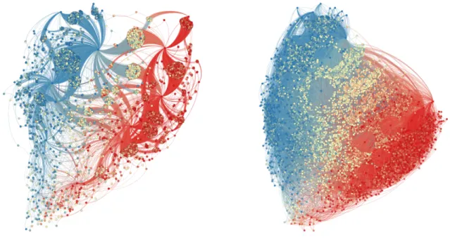
Figure 3: Left: A network of size 10000 generated with the undirected Strickland algorithm with F = 0.4, P = 1/2 making 2 connections per new node. Right: a network with the same parameters, but with 5 connections per new node. They both have a similar structure and shape, but the right hand plot has more complexity due to its increased number of connections. Blue nodes have traits near 0, red nodes have traits near 1, and yellow nodes have traits in the middle.

Figure 4: Left: A network of size 10000 generated with the undirected Strickland algorithm withF = 1/3, P = 1/2 making 2 connections per new node. Right: a network with the same parameters, but with 5 connections per new node.

The above plot illustrates the same situation as before but shifts the Global F to 1/3, which corresponds to a situation where every trait is equally likely. This can be seen by the roughly equal representation of each color in the plot. As before, the low number of connections in the right hand plot results in nodes grouping up based solely on which two supernodes they are connected to.

In figure 5, the trait distribution is a tight bell shape, so the majority of the nodes are very similar. As a result of this, any node is essentially equally likely to connect to any other node of similar degree, so the plot seems much more random. This reflects the fact that as the Global F approaches 0 our model tends to the Barab´asi-Albert algorithm. It is also a result of the assumption made in the model that decreased diversity increases tolerance, so connections between two nodes of differing traits are more likely relative to models with a largerF. There are a few nodes that fell far from the center of the bell curve, seen here as the blue node that have very few other nodes surrounding it. These nodes have very high degree due to an artifact of the beta distribution that means mid-trait nodes preferentially attach to nodes with extreme traits when F is small, however this is not an issue since in these scenarios, extreme trait nodes are rare.

It is important to quantify these results with numbers, which we will attempt to do below by comparing our results to some important metrics.

Notation:

N — final number of nodes in the network

m0 — size of initial seed network

m1 — number of connections made in the initial phase

P — the mean trait of the network

Clustering Coefficient

N m0 m1 Global F P Avg. Clustering Coefficient

1000 3 2 1/3 1/2 0.44

1000 3 2 1/4 1/2 0.17

1000 3 2 1/8 1/2 0.10

1000 3 5 1/3 1/2 0.37

1000 3 5 1/4 1/2 0.34

1000 3 5 1/8 1/2 0.10

The average clustering coefficient of a network generated by the Strickland algorithm shrinks as the Global F shrinks towards 0. This is likely because as the Global F decreases, the generated network becomes more and more random since there is an increased tendency to connect based only on degree as well as an increased tolerance. As a result, the neighborhoods of each node are essentially random, so the odds of a neighborhood being close to complete are low. On the other hand, a higher Global F results in situations like those shown in the plots above where most nodes are clustered around supernodes with a similar trait to their own. This stratification based on trait means that two nodes that are connected likely share a similar trait and are thus also likely to both be connected to the same supernode. This tendency increases the local clustering coefficient, boosting the global clustering coefficient as well. Increasingm1 also has the

effect of decreasing the clustering coefficient since it greatly expands the average neighborhood size, making neighborhood completeness far less likely.

Path Length

N m0 m1 Global F P Avg. Shortest Path Length

1000 3 2 1/3 1/2 2.46

1000 3 2 1/4 1/2 2.96

1000 3 2 1/8 1/2 3.46

1000 3 5 1/3 1/2 2.08

1000 3 5 1/4 1/2 2.09

Here we see that decreasing the Global F increases the average path length for similar reasons to the decrease in the clustering coefficient. More trait separated community means that most nodes in a community have a very short path to other nodes in the community. Decreasing the community by decreasing the Global F makes it less likely for there to be a short path along a common connection between two nodes. Further, increasingm1decreases the average path length since there are the same number of nodes but more

connections between them, so there is more likely to be a shorter path than before.

Degree Distribution

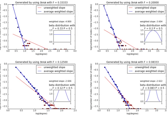
Below are several plots showing the degree distribution of some realizations of the Strickland algorithm. The log-log plot helpfully includes the global trait beta distribution in the bottom right corner. Note the plot’s heavy tail, which is a feature of complex social networks [15]. These plots represent only a single randomly-generated network, and as such they are not conclusive evidence of the properties of all networks sharing those parameters as a whole, although the behavior of networks with the same parameters are very similar in this regard. Each network consists of 10000 nodes and has aP of 0.5, a seed network of 3 nodes, and makes 2 connections per new node.

Figure 6: Log-log plots of degree distributions. The red dots indicate observations (there are many overlaps), and the blue dots indicate the average log-degree of the nodes with a given log-frequency. By doing this, linear regression on these averages deemphasizes the tail, giving us an idea of what theγvalue of the degree distribution is without the heavy tail. We do note, however, that linear regression has been criticized as a method for determiningγ, but here it suffices since the exact value ofγ is not our main interest [5].

Assortativity

Assortativity is given as a 95% confidence interval based on ten generated networks.

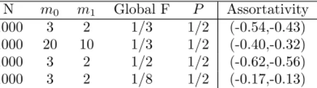
N m0 m1 Global F P Assortativity

1000 3 2 1/3 1/2 (-0.54,-0.43) 1000 20 10 1/3 1/2 (-0.40,-0.32) 1000 3 2 1/2 1/2 (-0.62,-0.56) 1000 3 2 1/8 1/2 (-0.17,-0.13)

The above table illustrates some of the effects the varying parameters have on the assortativity of the networks. Entries 1 and 2 show that increasing the number of connections per new node increases assorta-tivity. The first, third, and fourth entries show how decreasing the Global F increases assortaassorta-tivity. These phenomena will be explored in the following tables. Note that all of the assortativites generated by the undirected Strickland algorithm are negative. This is a major shortcoming of the model and had a heavy influence on the creation of the directed Strickland algorithm.

One of the other factors affecting assortativity is the Global F. As discussed, the Global F carries infor-mation about the biases of the members of the network since tolerance was defined as the complement of the Global F. It does so by changing the shape of the beta distribution that F-Traits are drawn from. A Global F of 1/3 means every F-Trait is equally likely. The distribution gets more bell shaped as the Global F tends to 0, and more U shaped as it increases to 1. Below are some examples:

N m0 m1 Global F P Assortativity

1000 3 2 3/5 1/2 (-0.70,-0.59) 1000 3 2 1/2 1/2 (-0.68,-0.61) 1000 3 2 1/3 1/2 (-0.51,-0.40) 1000 3 2 1/4 1/2 (-0.40,-0.26) 1000 3 2 1/8 1/2 (-0.17,-0.13)

This table shows how assortativity changes as the Global F decreases. As shown prior, the Barab´ asi-Albert model has an assortativity of 0, so it makes some sense that the assortativity of the Strickland algorithm is also approaching 0. Recall that assortativity is a measure of correlation between degrees of connected nodes. Thus, a negative assortativity indicates that low degree nodes are connected to high degree nodes and not each other, and likewise for nodes of high degree. This explains the very negative assortativity of the algorithm since the majority of nodes have low degree based on the power law distribution and yet they mostly connect to supernodes when the Global F is high, as seen in the example plots above.

N m0 m1 Global F P Assortativity

100 3 2 1/3 1/2 (-0.42,-0.35) 500 3 2 1/3 1/2 (-0.43,-0.33) 1000 3 2 1/3 1/2 (-0.52,-0.34) 5000 3 2 1/3 1/2 (-0.69,-0.54)

Here we explore the effect of network size on assortativity. There does seem to be a relationship between the two, which is troubling if we want to have consistent model behavior across network sizes.

Bootstrap

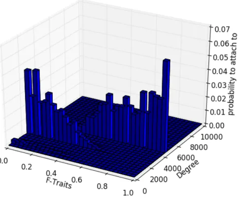
Figure 8: An example bootstrap for a network of 10000 nodes with a Global F of 0.4, a P of 0.5, a seed network of 3 nodes, and 2 connections made per new node.

The bootstrap represents the probability distribution for a randomly generated new node to attach to existing nodes. The plot seems to suggest that if the new node has a low F-Trait, it is very likely to connect to a node with a degree near 4000, and if it has a high F-Trait, it will likely connect to a node with degree near 7000. This suggests that there is a supernode with a high F-Trait that is absorbing all the connections made by new nodes with high F-Traits, and a few supernodes that are all also splitting up the connections made by new nodes with a low F-Trait. A similar phenomenon can be seen in figure 3 which has identical parameters.

4.3

Directed Strickland

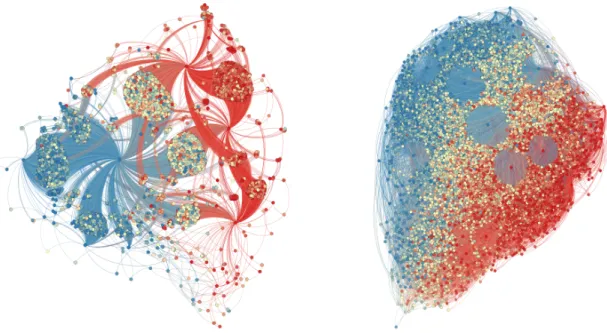
Figure 9: Left: A network of size 1000 generated with the directed Strickland algorithm with F = 0.4, P = 1/2 making 2 connections per new node in Phase 1, and 1 connection per new node in Phases 2 and 3. Right: a network with the same parameters, but with 5 connections per new node in Phase 1. Blue nodes have traits near 0, red nodes have traits near 1, and yellow nodes have traits in the middle.

Figure 10: Neighborhood of a node (center) of moderate degree taken from the previous plot.

We again try to quantify the visible results seen above with the tables below.

Notation:

N — final number of nodes in the network

m0 — size of initial seed network

m1 — number of connections made in the initial phase

m2 — number of connections made based solely on F-Trait

m3 — number of connections made in the friends of friends phase

P — the mean trait of the network

Clustering Coefficient

Below is a table of clustering coefficients for a few different realizations of the directed Strickland algo-rithm.

N m0 m1 m2 m3 Global F P Avg. Clustering Coefficient

1000 3 2 2 2 1/3 1/2 0.284

1000 10 5 5 5 1/3 1/2 0.231

1000 3 2 2 2 1/4 1/2 0.306

1000 3 2 2 2 1/2 1/2 0.281

1000 5 5 2 2 1/3 1/2 0.370

1000 5 2 5 2 1/3 1/2 0.148

1000 5 2 2 5 1/3 1/2 0.456

connection between the Global F and the clustering coefficient than in the undirected model. We are not sure what the specific cause for this is, but it could be because the directed Strickland model makes far more connections than the undirected model making the correlation coefficients lower across the board. The final three entries show the effect of each parameter on the clustering coefficient when considered in conjunction with the first entry. Increasing m1 increases the clustering coefficient since these connections are weighted

on degree, meaning that this phase is likely to result in a new node connecting to a supernode which is also likely to be connected to the neighbors of the new node, forming complete neighborhoods. Supernodes are also likely connected to each other due to Phase 4’s emphasis on connecting to like degrees. Increasingm2,

however, decreases the clustering coefficient since the new node is connecting to nodes based solely on trait, meaning they are likely to connect to nodes of small degree (the vast majority of nodes in the network) that are unlikely to be connected to the new node’s other neighbors. Finally, increasingm3vastly increases

the clustering coefficient. The reason for this is clear when one considers the nature of Phase 3. Phase 3 connects a new node to the friends of its friends — in other words, it fills out a new node’s neighborhood with many mutual connections, which is exactly what the clustering coefficient measures.

Path Length

N m0 m1 m2 m3 Global F P Avg. Shortest Path Length

1000 3 2 2 2 1/3 1/2 2.56

1000 10 5 5 5 1/3 1/2 2.18

1000 3 2 2 2 1/4 1/2 2.46

1000 3 2 2 2 1/2 1/2 2.64

1000 5 5 2 2 1/3 1/2 2.40

1000 5 2 5 2 1/3 1/2 2.50

1000 5 2 2 5 1/3 1/2 2.12

The results here are consistent with what we would expect from a social network — high clustering but short average path length. These results have fewer surprises. The average path length directly mimics the path length behavior for undirected Strickland networks. The only new behavior is how each of the new phase parameters affects the path length. The biggest effect comes from Phase 3. This change likely drops the average path length by shortening a path that was previously node→ friend→friend of friend to just node→friend of friend.

Degree Distribution

Figure 11: Log-log plots of degree distribution for different values of the Global F. These plots represent a single realization of the directed Strickland algorithm of size 1000 with 2 connections made in all three phases.

variation in degree for the directed Strickland model. This is because in the newly added phases many of the connections are optional and thus most nodes have slightly different degrees.

Assortativity

Assortativity is given as a 95% confidence interval.

N m0 m1 m2 m3 Global F P Assortativity

1000 3 2 2 2 1/3 1/2 (-0.10,-0.08) 1000 20 10 20 10 1/3 1/2 (0.02,0.04) 1000 10 3 10 3 1/2 1/2 (0,0.02) 1000 20 5 18 5 1/8 1/2 (0.31,0.32)

Compare this table with the first table for undirected networks and it is clear that the directed Strickland algorithm produces a far more realistic assortativity. In subsequent tables we will see the role that each parameter plays in determining the assortativity of a network.

The following table is a demonstration of how a small perturbation in each of the parameters affects the final assortativity in the final model:

N m0 m1 m2 m3 Global F P Assortativity

1000 10 2 2 2 1/3 1/2 (-0.10,-0.08) 1000 10 5 2 2 1/3 1/2 (-0.10,-0.07) 1000 10 2 5 2 1/3 1/2 (0.27,0.31) 1000 10 2 2 5 1/3 1/2 (-0.27,-0.23)

We see that compared to the benchmark of the first test,m1, the number of out-connections made in the

initial phase, has little effect on the assortativity. This insignificance makes sense since this phase mostly targets supernodes, thus changing the in-degree of relatively few nodes. The second test shows that making more connections based on F-Trait similarity vastly increases our assortativity. The huge effect is caused by the fact that a high m2value lets new nodes (which are always of low degree) connect with other nodes

without concern for degree. Since the vast majority of nodes in the network are of low degree, this lets small degree nodes connect to other small degree nodes which raises our assortativity. Finally, making more friends of friends connections brings assortativity down, which also makes intuitive sense since in this phase the connections are made based on popularity of friends of friends, meaning a new, low degree node is most likely to connect to a node of much higher degree, lowering assortativity.

Another interesting result that can be seen through testing is the non-linearity of the effects of our parameter changes. As seen in the table below, by making an identical change to each of the parameters, we are still able to change the assortativity. This suggests that the decreases caused by increasing m3 are

outstripped by the effect of increasingm2.

N m0 m1 m2 m3 Global F P Assortativity

1000 10 2 2 2 1/3 1/2 (-0.10,-0.08) 1000 10 5 5 5 1/3 1/2 (0.02,0.05) 1000 10 7 7 7 1/3 1/2 (0.09,0.11)

N m0 m1 m2 m3 Global F P Assortativity

1000 3 2 3 2 3/4 1/2 error

1000 3 2 3 2 1/2 1/2 (-0.09,-0.08) 1000 3 2 3 2 1/3 1/2 (-0.08,-0.07) 1000 3 2 3 2 1/4 1/2 (-0.08,-0.02) 1000 3 2 3 2 1/8 1/2 (0.01,0.06)

Another factor affecting this trait distribution is the P parameter, which informs the expected value of the beta distribution. AP parameter of 1/2 means the distribution is symmetric. This is theP parameter that was used for all tests. Further exploration of the effect this parameter has could be an interesting next step.

In modeling real social network changes, we feel that examining changes to the Global F and P param-eters could provide interesting results, once realistic values for m1, m2, m3 are determined. Holding all else

constant, shifting the Global F slowly higher could be used to study the effects on a community of people where political ideals are becoming increasingly polarized. In the same vein, shifting the P value could be used to model a population where a more radical idea is slowly becoming the norm, leaving a “tail” of people whose views have not shifted. A challenging but potentially informative extension of the Strickland algorithm would be a model where the Global F or P could gradually shift at a user specified speed in a user specified directionwhile the network is being built, or perhaps introducing random perturbations that might have a snowballing effect on the community.

The following table shows the association between assortativity and the size of the network.

N m0 m1 m2 m3 Global F P Assortativity

100 10 2 3 2 1/3 1/2 (-0.4,0.6) 500 10 2 3 2 1/3 1/2 (-0.08,-0.03) 1000 10 2 3 2 1/3 1/2 (-0.08,-0.07) 5000 10 2 3 2 1/3 1/2 (-0.11,-0.08)

The confidence intervals appear to be much wider for smaller values ofN, which is not too unexpected as individual deviations can have a larger effect when there are fewer nodes. Beyond that, the assortativities seem to be mostly unaffected by scale, a difference between the directed and undirected algorithms that is promising, since this version of the algorithm seems to be less affected by scaling.

Assortativity Final Thoughts

Figure 12: Comparison of different assortativites for social networks [8].

The two social networks are the Leadership network, a graph of positive sentiment between students in a leadership class, and the Prison network, which also shows positive sentiment among prisoners. Note that this diagram plots assortativity type vs ASP, which is a normalized Z-score showing how much a network’s assortativity deviates from what is expected. This paper therefore suggests that in the future it could be interesting to see how the other forms of directed assortativity for Strickland algorithm generated networks compare to what is typical for a social network. However, our cursory exploration suggests the various forms of directed assortativity are all about the same for the directed Strickland algorithm.

A New Metric

After considering the various permutations of in/out degree assortativity, we decided to consider a new metric for assortativity that would hopefully give us more insight into the structure of our networks. We took our existing directed network and created an undirected network from it by replacing every bidirectional connection with an undirected edge and leaving no edge for connections between nodes that were strictly unidirectional. We then calculated the assortativity of this new network, however, we used the in-degree of the nodes in the original, directed graph in place of the degree of the newly created undirected graph. This calculation was done using networkx.attribute assortativity coefficientand a stored dictionary of in-degrees from the directed network. We called this metric the bidirectional assortativity. The idea behind the creation of this metric was to determine whether there was any correlation between the popularities of friends. We found that for every network generated by the final Strickland algorithm, the resulting bidirectional assortativity was 0. We also applied this metric to two real world social networks, the Pokec network (discussed later) and a network of sent emails in an academic institution, and found that these networks also had a bidirectional assortativity of nearly 0. No further work was done examining the properties of other networks’ bidirectional assortativity, but it could be interesting grounds for further exploration.

5

Summary and Next Steps

results, and might help the undirected assortativity. There are three main directions that we would like to take the project from here. Firstly, more work should be done with the directed algorithm to fit it to real social networks. Some preliminary work was done with the Pokec network, a 1.6 million node directed social network from a Slovakian social media site. This network also has more than a dozen different parameters attached to each account — location, age, education level, etc. — making this network an ideal candidate for comparison. However, so far only superficial properties of the network have been calculated (directed assortativity, clustering coefficient, etc.). In future work, realistic parameters should be determined for this network so a Strickland algorithm generated model can be created to see if the algorithm generates networks with similar properties. Additionally, there are several other metrics, such as the eleven mentioned in [1] that it would be useful to compare our model to. Secondly, the original Strickland algorithm is very similar to the Barab´asi-Albert model, which has rigorous proof of its asymptotic power law distribution. This proof makes use of master equations, and a similar approach may be applicable to the undirected version of the Strickland algorithm. Having a rigorous proof of the properties of the Strickland algorithm would be highly desirable. Finally, the greatest advantage of the Strickland algorithm is its ability to be extended in an intuitive way to a multi-trait space. This is potentially rich ground for exploration since real social networks certainly have more depth than just a single trait space.

6

Acknowledgements

References

[1] Leman Akoglu and Christos Faloutsos. Rtg: A recursive realistic graph generator using random typ-ing. In Wray Buntine, Marko Grobelnik, Dunja Mladeni´c, and John Shawe-Taylor, editors, Machine Learning and Knowledge Discovery in Databases, pages 13–28, Berlin, Heidelberg, 2009. Springer Berlin Heidelberg.

[2] R´eka Albert and Albert-L´aszl´o Barab´asi. Statistical mechanics of complex networks.Reviews of modern physics, 74(1):47, 2002.

[3] David J. Balding and Richard A. Nichols. A method for quantifying differentiation between populations at multi-allelic loci and its implications for investigating identity and paternity. Genetica, 96(1):3–12, 1995.

[4] Deepayan Chakrabarti and Christos Faloutsos. Graph mining: Laws, generators, and algorithms. ACM Comput. Surv., 38(1), June 2006.

[5] A. Clauset, C. Rohilla Shalizi, and M. E. J. Newman. Power-law distributions in empirical data. ArXiv e-prints, June 2007.

[6] P. Erd˝os and A. R´enyi. On random graphs i. Publicationes Mathematicae (Debrecen), 1959.

[7] P. Erd˝os and A. R`enyi. On the evolution of random graphs. 1960.

[8] Jacob G. Foster, David V. Foster, Peter Grassberger, and Maya Paczuski. Edge direction and the structure of networks. Proceedings of the National Academy of Sciences, 107(24):10815–10820, 2010.

[9] E. N. Gilbert. Random graphs. Ann. Math. Statist., 30(4):1141–1144, December 1959.

[10] Martin Grandjean. A social network analysis of twitter: Mapping the digital humanities community.

Cogent Arts & Humanities, 3(1):1171458, 2016.

[11] A. Hashmi, F. Zaidi, A. Sallaberry, and T. Mehmood. Are all social networks structurally similar? a comparative study using network statistics and metrics. ArXiv e-prints, October 2013.

[12] Stuart Koschade. A social network analysis of ”jemaah islamiyah”: The applications to counterterrorism and intelligence. Studies in Conflict & Terrorism, 29(6):559–575, 2006.

[13] M. E. J. Newman. Assortative mixing in networks. Physical review letters, 89(20):208701, 2002.

[14] M. E. J. Newman. The structure and function of complex networks.SIAM Review, 45(2):167–256, 2003.

[15] Steven H. Strogatz. Exploring complex networks. Nature, 410(6825):268–276, 2001.

[16] Saatviga Sudhahar, Gianluca De Fazio, Roberto Franzosi, and Nello Cristianini. Network analysis of narrative content in large corpora. Natural Language Engineering, 21(1):81112, 2015.