Sharif University of Technology
Scientia IranicaTransactions E: Industrial Engineering http://scientiairanica.sharif.edu
An improved model and heuristic for capacitated
lot-sizing and scheduling in job shop problems
O. Poursabzi, M. Mohammadi
, and B. Naderi
Department of Industrial Engineering, Faculty of Engineering, Kharazmi University, Tehran, Iran. Received 26 June 2016; received in revised form 29 July 2017; accepted 25 December 2017
KEYWORDS Lot-sizing and scheduling; Job shop;
Sequence-dependent; Lower bound; Heuristic.
Abstract. This paper studies the problem of capacitated lot-sizing and scheduling in job shops with a carryover set-up and a general product structure. After analyzing the literature, the shortcomings are easily realized; for example, the available mathematical model is unfortunately not only non-linear, but also incorrect. No lower bound and heuristic are developed for the problem. Therefore, we rst develop a linear model for the problem in hand. Then, we adapt an available lower bound in the literature to the problem studied here. Since the problem is NP-hard, heuristic based on production shifting concept is also proposed. Numerical experiments are used to evaluate the proposed model and algorithm. The proposed heuristic is assessed by comparing it with other algorithms in the literature. The computational results demonstrate that our algorithm has an outstanding performance in solving the problem.
© 2018 Sharif University of Technology. All rights reserved.
1. Introduction
Production management is a multi-disciplinary task simultaneously involving many factors. Lot-sizing and scheduling are the two main parts of production planning and control system. Lot-sizing deals with determining the production amount of each product at each production run, often over a nite multi-period horizon. A lot indicates the quantity of a given product processed on a machine continuously without interruption after its correspondent set-up. On the other hand, scheduling is to determine the production sequence in which the products are manufactured on a single machine [1].
The integrated problem provides a more
eec-*. Corresponding author.
E-mail addresses: [email protected] (O. Poursabzi); [email protected] (M. Mohammadi); bahman [email protected] (B. Naderi)
doi: 10.24200/sci.2017.20016
tive production plan than the cases in which two problems are solved hierarchically by inducing the solution to the lot-sizing problem in the scheduling level. Simultaneous lot-sizing and scheduling is essen-tial, especially when sequence-dependent set-up costs and times occur [2]. In many of the production environments, switching between production lots of two dierent products triggers operations such as machine adjustments, tool changing, and cleansing procedures. These set-up operations are usually dependent on the sequence [2]. In order to avoid unnecessary changeovers, customer demand has to be pooled in the production orders (lots). When sequence-dependent set-up times are predominant, the available capacity for production depends on both sequence and size of the lots. In such a situation, lot-sizing and scheduling have to be applied simultaneously [3]. Consequently, the production sequence must be explicitly embedded in the lot denition and scheduling.
The problem of the integrated lot-sizing and scheduling can be either capacitated or incapaci-tated [4]. Another issue in this area is the product
structure. In one type, only a set of nal products are planned, while in another one, assembly products are assumed [2]. That is, each nal product is the assembly of some other intermediate products and it can be manufactured when all its intermediate products are planned. In the assembly type, the products can have either serial or general structure. In the serial structure, each product has only one predecessor and one successor, while in the general one, each product can have multiple predecessors and successors. If each product needs one operation for completion, the prob-lem is called single-level, while if it requires more than one operation, the problem is dened as multi-level. In the case of multi-level operation, when all the products have the same processing route, the problem is called a ow shop; while when each one has its own unique processing route, the problem is called a job shop.
The incapacitated problem has been well studied in the literature. The incapacitated lot-sizing ow shop was reviewed by Ouenniche and Bertrand [5], while the incapacitated lot-sizing job shop was studied by Ouen-niche et al. [6]. Regrding the capacitated problems, the rst conclusion is that the papers focus more on the ow shops than on the job shops. In this regard, one can refer to Maravelias and Sung [7], Karimi-Nasab and Seyedhoseini [8], Stadtler and Sahling [9], and Babaei et al. [10].
Mohammadi et al. [11] considered the ow shop-based lot-sizing and scheduling problem and proposed a Mixed Integer Linear Programming (MILP) model. Their model was an extension of the model previously proposed for the parallel-machine version of the ow shop-based lot-sizing and scheduling problem [12]. Later, the same authors proposed several rolling hori-zon heuristics in [11,13] and a Genetic Algorithm (GA) was extended by Mohammadi et al. [14,15] for the same problem. Mohammadi and Jafari [16] also developed the mentioned problem with parallel machines at each stage. They proposed a Lower Bound (LB) as well as a mixed integer programming-based algorithm. Rameza-nian et al. [17] developed an improved mathematical model for the same problem proposed by Mohammadi et al. [15]. Ramezanian and Saidi-Mehrabad [18] devel-oped the problem with stochastic processing times and proposed a Mixed Integer Programming (MIP) model. Considering the importance of lot-zing and scheduling of the job shop manufacturing systems, this issue has less been studied than the ow shop systems. Hence, we will present a review of this issue in the following.
Karimi-Nasab and Seyedhoseini [8] studied the job shop-based problem, but they ignored carryover set-up times. More importantly, they only considered scheduling of nal products and ignored the general product structure. Moreover, Fandel and Hegene [2] generalized the problem with both carryover set-up
and general product structure and proposed a math-ematical model for the problem. Unfortunately, this model does not work correctly. More detail on why the model is incorrect is presented in Section 2. Besides its incorrectness, the model of Fandel and Stammen-Hegene [2] is non-linear. Authors did not propose solution method to solve the problem.
Lasserre [19] and Dauzere-Peres and Lasserre [20] presented integrated models of product, multi-period job shop lot-sizing and scheduling problems considering set-up scheduling for the job shop man-ufacturing system. Since this problem was NP-hard, they oered a decomposition approach in which a production planning problem with a xed sequence of products on machines was considered at rst and then, based on this xed production plan, scheduling was carried out using an adapted version of Shifting Bottleneck algorithm.
Lalitha et al. [21] studied N-stage hybrid ow shop lot streaming problem for the multi-product single-period case. The aim was to minimize the makespan. In this regard, they tried to respond to the following issues: quantity of sub-lots, sequence of sub-lots, and jobs. Since the problem was NP-hard, they developed a heuristic algorithm for large-scale instances. Giglio et al. [22] studied a lot-sizing and scheduling problem considering energy consumption with the goal of minimizing total cost of the system. They solved a single-level multi-period problem and considered xed set-up parameters. They also im-plemented a relax-and-x based heuristic algorithm. Wolosewicz et al. [23] considered a constant sequence for the operations in the lot-sizing and scheduling problem with constant set-up. They developed an adaptation of Lagrangian methods for the large-scale instances. Karimi-Nasab et al. [24] considered a lot-sizing and scheduling problem with compressible processing time. They considered a constant sequence of jobs, where by allocating the jobs to each machine, the lot size of jobs would be determined. Also, their solution procedure was a variation of Particle Swarm Optimization (PSO). Karimi-Nasab et al. [25] investi-gated simultaneous lot-sizing and scheduling problem in a job shop manufacturing environment over a nite number of periods. They supposed that each machine could operate at dierent discrete speed levels and the set of modes for each machine was known in advance. The problem was formulated as an Integer Linear Program (ILP) and a branch and cut approach was employed so as to solve it. The goal was to minimize the total costs originating from set-up, production, inventory holding, and shortage. Urrutia et al. [26] incorporated both lot-sizing and scheduling problems simultaneously and considered sequence-independent set-up time/cost, single level, and multiple items. In order to solve the problem, they considered a constant
sequence of jobs and solved their models using an adaptation of Lagrangian method. They made an endeavor to solve the lot-sizing problem at rst and then tried to improve the sequence of jobs. Mateus et al. [27] studied a constrained lot-sizing and schedul-ing problem under sschedul-ingle-level manufacturschedul-ing system, unrelated parallel machines, and sequence-dependent set-up conditions. They optimized their solution as separable (independent) consequent processes. First, lot sizes were calculated and then, the scheduling problem was solved using GRASP method. Finally, a new methodology was presented so as to combine both solutions together. Zhang and Yan [28] proposed a non-linear mathematical model for the product multi-period simultaneous lot-sizing and scheduling problem, in which the type of set-up was simple and only end products were taken into account. They also deployed a GA to solve the problem in hand. Ouenniche and Boctor [29] proposed a multi-stage approach to nd a solution to the lot-sizing and scheduling problem. They rst determined the scheduling by solving a non-linear model and then, calculated lot sizes based on the given schedules. For the medium and large-scale problems, they implemented Simulated Annealing (SA) and Tabu Search (TS) algorithms. In their model, the demand of customers was deterministic and set-ups were independent from sequences.
After a detailed review of the literature, the existing research gap motivated the authors to study the problem of job shop-based lot-sizing and scheduling so as to overcome the current shortcomings in the literature. This paper rst presents a mixed integer, interestingly linear, programming model and both the problem and the model are then analyzed to introduce an eective LB. Moreover, production shifting-based heuristic is proposed so as to solve the problem. The proposed model, LB, and heuristic are evaluated through several numerical experiments.
The rest of the paper is organized as follows: Section 2 denes and formulates the problem in hand. Section 3 presents the proposed LB, while Section 4 proposes a production shifting-based heuristic. Then, Section 5 conducts numerical experiments to evaluate the proposed model, LB, and heuristic. Finally, Section 6 provides conclusions and future research directions.
2. Problem denition and formulation
The problem under consideration can be described as follows. There is a set of N products and a set of M ma-chines for production. On the one hand, the products are assumed to follow the general product structure (i.e., they are assembly products and each part might have more than one predecessor and successor). The lower-level products are the elements of the higher-level
ones. Therefore, the production of the upper levels can be started when all of its elements at the lower levels are already produced. Also, the products are assumed to be multi-level; that is, each product needs multiple operations for completion. Each operation is carried out with one machine and the processing route of each product diers from the others. Note that one operation can be started when its precedent operation is already nished, called vertical interaction.
The planning horizon is nite, consisting of T macro-periods of the same length. For each product, there may be both external (independent) and internal (dependent) demands. The nal products have only external demands. The demands for each period have to be satised during that period. Thus, no shortage is allowed. Moreover, each product can be produced at most as a single lot during each period.
In this production system, we assume that ma-chines are capacitated as resources. The set-up is also assumed to be sequence-dependent (i.e., its magnitude and cost depend on product sequence) and carry-over (i.e., it can be accomplished within the next micro-period). Each macro-period is segmented into several micro-periods (see Figure 1), in which the rst micro-period is also assigned to the set-up process. Regarding the precedence relations and the general product structure, some standstills may occur during the process, of which the length can be measured using the shadow product concept. Each product cannot be produced on more than one machine and each machine cannot process more than one product in a micro-period. It is also assumed that machines are continuously available.
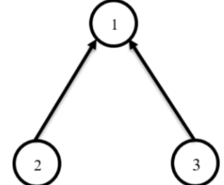
The integrated lot-sizing and scheduling problem is concerned with determining the periods in which all products are manufactured, their lot size, and product sequence on each machine, simultaneously. The objective is to minimize the cost of the network including set-up, production, inventory, and idle costs. For further illustration, a numerical example is presented. Consider a job shop problem with three products and two machines including two planning
Figure 1. The product structure for the example with N = 3.
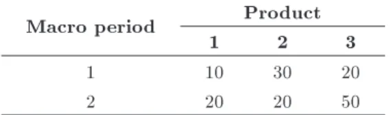
Table 1. The demands for the numerical example.
Macro period Product
1 2 3
1 10 30 20
2 20 20 50
horizons and two macro-periods. Figure 1 and Table 1 show the three product structures and demands, re-spectively. The processing route is as follows:
Product 1 = f1; 2g; Product 2 = f2; 1g; and Product 3 = f2g:
Also, the processing and set-up costs are as follows: b1= 2; b2= 3; b3= 1; w1;3=w3;1=30;
w1;2 = w2;1 = 20; w2;3 = w3;2 = 10:
A feasible solution for this example is shown in Fig-ure 2. The numbers on the arcs signify the quantity of the lower-level products.
The indices, parameters, and variables of the multi-level general lot sizing and scheduling problem (MLGLSP) MM are shown below:
Indices:
i; j; k; l; n Product or item type;
f Micro-periods per machine in each macro-period;
; A specic micro-period per machine in each macro-period in accordance with the micro-period segmentation of the machine;
m; m Machine type; T Macro-period. Parameters:
T Planning horizon;
N Number of dierent products; M Number of dierent machines
(or dierent stages) available for production;
aji Production coecient, which indicates
how many units of product j are required to produce a unit of product i;
BM A large number;
bj;m Capacity of machine m required for
the production of a unit of product j (in time units per quantity unit); ~bj;m Capacity of machine m required as
input in order to produce one unit of the shadow product j (in time units per quantity unit), also referred to as the input coecient;
Cm;t Available capacity of each machine m
in macro-period t (in time units); dj;t External demand for product j at
the end of macro-period t (in units of quantity);
hj;t Storage costs unit rate for product j in
macro-period t;
oj;m Cost unit rate for maintaining the
set-up condition of machine m for product j (in money units per time unit);
pj;m;t Production costs for producing one
unit of product j on machine m in the macro-period t (in money units per quantity unit);
Sij;m Sequence-dependent set-up costs
for the set-up of machine m from the production of product i to the production of product j (in money units); to i 6= j, sij;m 0 applies and
for i = j, sij;m= 0;
wij;m Sequence-dependent set-up times
for the set-up of machine m from the production of product i to the production of product j (in time units); to i 6= j, wij;m 0 applies and
for i = j, wij;m = 0.
Variables
Ij;0 Stock of product j at the start of the
planning horizon (in quantity units); Ij;T Stock of product j at the end of the
planning horizon (in quantity units); qj;m;f;t Production quantity of product j in
the micro-period f of macro-period t on machine m (in quantity units); ~qj;m;f;t Quantity of shadow product j in the
micro-period f of macro-period t on machine m (in quantity units); zj;m;f;t A binary variable which indicates
whether micro-period f of macro-period t is an idle macro-period for machine m in which the set-up condition for product j is maintained (zj;m;f;t = 1)
or not (zj;m;f;t = 0); with zj;m;f;t= 1,
product j has the role of a shadow function.
Decision variables
xij;m;f;t A binary variable which indicates
whether to set up machine m from the production of product i to the production of product j in micro-period f of macro-micro-period t on machine m (xij;m;f;t= 1) or not (xij;m;f;t= 0);
yj;m;f;t A binary variable which indicates
whether machine m is set up (yi;m;f;t = 1) or not (yi;m;f;t = 0) in
micro-period f of macro-period t for the production of product j.
The MILP formulation of the problem is as follows (Eqs. (1)-(20)):
Objective function: min XN
i=1 N X j=1 M X m=1 T X t=1 3 X f=1
NSij;m:xij;m;f;t
+XN
j=1 T
X
t=1
hj;t:Ij;t+ N X j=1 M X m=1 T X t=1 3N X f=1
pj;m;t:qj;m;f;t+ oj;m:~bj;m:~qj;m;f;t
: (1) Subject to:
Ij;t=Ij;t 1+ M X m=1 3N X f=1 qj;m;f;t N X i=1 M X m=1 3N X f=1
aji:qi;m;f;t dj;t;
j = 1; ; N; t = 1; ; T; (2) [aji]
"
BM(yj; m;;t 1) +
"
bj; m:qj; m;;t
+ XN
n=1;n6=j 1
X
=1
bn; m:qn; m;;t
+
N
X
k=1;k6=n
xnk; m:;t:wnk; m+ ~bn; m:~qn; m;;t
!##
[aji]
"
BM(1 yi;m;f;t)
+ XN
n=1;n6=i f 1X =1
bn;m:qn;m;;t;
+ XN
k=1;k6=n
xnk;m;;t:wnk;m+ ~bn;m:~qn;m;;t
!# ; j = 1; ; N; i 6= j; m; m = 1; ; M; f; = 1; ; 3N; t = 1; ; T; (3)
N X j=1 3N X f=1
bj;mqj;m;f;t+ N X i=1 N X j=1 j6=i 3N X f=1
wij;m:xij;m;f;t
+ N X j=1 3N X f=1
~bj;m:~qj;m;f;t= Cm;t;
m = 1; ; M; t = 1; ; T; (4) qj;m;f;tCbm;t
j;m:yj;m;f;t; j = 1; ; N;
m = 1; ; M; t = 1; ; T;
f = 1; ; 3N; (5)
~qj;m;f;tC~bm;t
j;m:zj;m;f;t; j = 1; ; N;
m=1; ; M; t=1; ; T; f =1; ; 3N; (6)
3N
X
f=1
yj;m;f;t 1; j = 1; ; N;
m = 1; ; M; t = 1; ; T; (7)
M
X
m=1
yj;m;f;t 1; j = 1; ; N;
f = 1; ; 3N; t = 1; ; T; (8)
N
X
j=1
0 B
@yj;m;f;t+ N
X
i=1 i6=j
xij;m;f;t+ zj;m;f;t
1 C A = 1;
m=1; ; M; t=1; ; T; f =2; ; 3N; (9) yj;m;(f 1);t+ xij;m;(f 1);t+ zj;m;(f 1);t
=yj;m;f;t+ xjk;m;f;t+ zj;m;f;t;
i; j; k = 1; ; N; i 6= j; j 6= k; m = 1; ; M; t = 1; ; T;
f = 3; ; 3N; (10)
yj;m;3N;(t 1)+ xij;m;3N;(t 1)
+ zj;m;3N;(t 1)= N
X
k=1
xjk;m;1;t;
i; j = 1; ; N; i 6= j;
m = 1; ; M; t = 2; ; T; (11) qj;m;f;t Cbm;t
j;m:(2 yj;m;f;t yj;m;(f 1);t);
j = 1; ; N; m = 1; ; M;
t = 1; ; T; f = 2; ; 3N; (12) ~qj;m;f;t C~bm;t
j;m:(2 zj;m;f;t zj;m;(f 1);t);
j = 1; ; N; m = 1; ; M;
t = 1; ; T; f = 2; ; 3N; (13) yj;m;f;t BM:
N
X
i=1 f 1
X
=1
xij;m;;t
! ; j = 1; ; N; m = 1; ; M;
t = 2; ; T; f = 2; ; 3N; (14)
N
X
I=1 N
X
j=1
xij;m;1;t 1; m = 1; ; M;
t = 1; ; T; (15)
Ij;0 = Ij;T = 0; j = 1; ; N (16)
yj;m;f;t2 f0; 1g; j = 1; ; N;
m = 1; ; M; t = 1; ; T;
f = 1; ; 3N; (17)
xij;m;f;t2 f0; 1g; i; j = 1; ; N;
m = 1; ; M; t = 1; ; T;
f = 1; ; 3N; (18)
zj;m;f;t2 f0; 1g; j = 1; ; N;
m = 1; ; M; t = 1; ; T;
f = 1; ; 3N; (19)
Ij;t; qj;m;f;t; ~qj;m;f;t 0; j = 1; ; N;
m = 1; ; M; t = 1; ; T;
f = 1; ; 3N: (20)
In this model, Eq. (1) represents the objective function which minimizes the sum of the sequence-dependent set-up costs, the storage costs, the production costs, and the costs of maintaining set-up conditions of the machine in the planning horizon. Constraint (2) ensures the balance of demand supply in each period. Two types of product's demand are taken into account in this model:
1. The external demand for products that must be provided at the end of each macro-period;
2. The internal demand of the products required for the production of high-level products in the product structure, which must be satised within the macro-period.
The external demand (dj;t) and the internal demand
(PNi=1PMm=1P3Nf=1aji:qi;m;f;t) of a macro-period for
product j must be provided by the previous macro-period's stock and the production quantity of product j in the current macro-period. Here, the rst period is exception, since the demands have to be provided by production.
Constraint (3) is used so as to consider vertical interaction in the proposed model. In this equation,
each typical product is produced before its direct substitute product in one macro-period. The left side of Constraint (3) is equal to the time between the beginning of the macro-period t and the end of the production of product j if micro-period f is a production micro-period for product j; otherwise, it is zero. In other words, if the value is not positive, the left side of Constraint (3) becomes zero. The right side of Constraint (3) is equal to the time between the beginning of period t and the beginning of the production of product i if micro-period f is a production micro-period for product i, or else it is a big number. In other words, if the value is positive, the right side of Constraint (3) is zero.
Constraint (4) shows the capacity constraints of machines during a macro-period. Constraint (5) indicates the relation between set-up and production processes and obtains an Upper Bound (UB) for production quantity. Constraint (6) determines the duration of idle times. It also yields a UB for the duration of the idle times. Constraints (7) and (8) guarantee that in each macro-period, at most a single lot is produced for each product. To achieve this aim, Fandel and Stammen-Hegene [2] applied:
M
X
m=1 lm
t
X
fm t =1
yj;m;fm t ) 1;
j = 1; ; N; t = 1; ; T;
but these constraints could not satisfy it. Assume a problem with N = 2, M = 3, T = 2, lm
t = 2,
Product routf1g = f1; 3g, and Product routf2g = f1; 2; 3g. Also, suppose that all products must be produced in period 1; then:
t = 1; lm t = 2 :
if j = 1; y1;1;1+ y1;1;2+ y1;2;1+ y1;2;2
+ y1;3;1+ y1;3;2 1;
if j = 2; y2;1;1+ y2;1;2+ y2;2;1+ y2;2;2
+ y2;3;1+ y2;3;2 1:
Due to the above expanding equation, for each product in each period, only one stage of product rout can be run on, so the products demand cannot be satised. However, by applying Eqs. (21) and (22) in the pro-posed model, the mentioned deciency is rectied.
t = 1; j = 1;
if m = 1; y1;1;1;1+ y1;1;2;1+ y1;1;3;1
+ y1;1;4;1+ y1;1;5;1+ y1;1;6;1 1;
if m = 2; y1;2;1;1+ y1;2;2;1+ y1;2;3;1
+ y1;2;4;1+ y1;2;5;1+ y1;2;6;1 1;
if m = 3; y1;3;1;1+ y1;3;2;1+ y1;3;3;1
+ y1;3;4;1+ y1;3;5;1+ y1;3;6;1 1: (21)
t = 1; j = 1;
if f = 1; y1;1;1;1+ y1;2;1;1+ y1;3;1;1 1;
if f = 2; y1;1;2;1+ y1;2;2;1+ y1;3;2;1 1;
if f = 3; y1;1;3;1+ y1;2;3;1+ y1;3;3;1 1;
if f = 4; y1;1;4;1+ y1;2;4;1+ y1;3;4;1 1;
if f = 5; y1;1;5;1+ y1;2;5;1+ y1;3;5;1 1;
if f = 6; y1;1;6;1+ y1;2;6;1+ y1;3;6;1 1: (22)
Constraints (9)-(11) bound the micro-periods in each macro-period to one of the following three positions: production, set-up, and idle micro-period.
To ensure this purpose, Fandel and Stammen-Hegene [2] presented the following equation in their paper:
N
X
i=1 N
X
j=1;j6=i
(yj;m;ft
m+ xij;m;fmt + zj;m;fmt ) = 1;
m = 1; ; M; t = 1; ; T; ft
m= 1; ; ltm:
In the case with m = 1, lm
t = 2, t = 1, and M = 3,
the generated constraint could be written as follows: if i = 1 then j = 2; 3 ! y2;1;2+ x1;2;1;2
+ z2;1;2+ y3;1;2+ x13;1;2+ z3;1;2;
if i = 2 then j = 1; 3 ! y1;1;2+ x21;1;2
+ z1;1;2+ y3;1;2+ x2;3;1;2+ z3;1;2;
if i = 3 then j = 1; 2 ! y1;1;2+ x31;1;2
+ z1;1;2+ y2;1;2+ x32;1;2+ z2;1;2;
2y1;1;2+ 2y2;1;2+ 2y3;1;2+ x1;2;1;2+ x1;3;1;2
+ x2;1;1;2+ x2;3;1;2+ x3;1;1;2+ x3;2;1;2
In contrast, the generated form of Eq. (9) can be written as:
if j = 1 then i = 2; 3 ! y1;1;2+ x21;1;2
+ x31;1;2+ z1;1;2;
if j = 2 then i = 1; 3 ! y2;1;2+ x21;1;2
+ x32;1;2+ z2;1;2;
if j = 3 then i = 1; 2 ! y3;1;2+ x13;1;2
+ x23;1;2+ z3;1;2;
y1;1;2+ y2;1;2+ y3;1;2+ x12;1;2+ x13;1;2+ x21;1;2
+ x23;1;2+ x31;1;2+ x32;1;2+ z1;1;2
+ z2;1;2+ z3;1;2= 1: (23)
The above-mentioned expression shows that:
i. According to this constraint, none of the micro-periods can be allocated to the production process. Therefore, considering the whole model, only the rst micro-period of each macro-period has the chance to implement the product process, which is against the innovation of the presented model, namely, the Big Bucket. The reason is that if it is impossible to produce more than one type of product in each macro-period, the Big Bucket assumption is violated;
ii. According to this constraint, after the second micro-period, no other idle micro-period would exist, which is very important for the whole model, especially for observing the vertical interaction. For example, assume that two products with direct precedence relation are produced in macro-period. To guarantee vertical interaction, an interval be-tween two micro-periods may be needed. It may also be much more commodious to keep the ma-chine ready for producing a specic product than producing one product at rst and then reverting the machine to the previous state. This constraint prevents the mentioned diculty;
iii. It is obvious that only the indicated variables in the set-up micro-periods can be 1. This constraint imposes consecutive set-up micro-periods on the model without any production process and conse-quently, enormous cost is imposed on the whole system.
In this paper, in order to observe the assumptions and to meet them along with the above-mentioned purposes, the equation in the research of Fandel and Stammen-Hegene [2] is replaced with Eq. (23).
Constraint (12) along with Constraints (7) and (8) determines that if one lot belonging to each product is produced in a macro-period, it must be produced within a micro-period, not in two or more directly successive micro-periods. Constraint (13) applies the same restriction for the standstill of the machine. Constraints (14) and (15) consider the set-up of the machine. Constraint (16) species that there is no on-hand inventory at the beginning/end of the planning horizon. Finally, Constraints (17)-(20) dene the type of decision variables.
2.1. Lower bound adaptation
Since the problem in hand in this research is NP-hard, providing LBs could be useful and applicable. For example, they can be a base point for approx-imation methods of evaluation; thus, the available LB is developed and employed. To do so, rst, the performance of the LB and model is assessed and then, the performance of the proposed heuristic is evaluated with respect to the LB. The adapted LB is taken from Mohammadi et al. [13] and obtained through linear relaxation of all binary variables in the model and adding Eq. (24):
3N
X
f=1
yj;m;f;t= Aj;m;t; j = 1; ; N;
m = 1; ; M; t = 1; ; T: (24) Aj;m;t is a binary variable.
Eq. (24) similar to a part of Eq. (23) has always been established in the original model.
After relaxing the binary variables, neither Eq. (3) nor (14) has signicant inuence on the model, since the left side of Eq. (3) would be a big negative number and the right side of Eq. (3) or (14) would be a big positive number owing to the values of the relaxed variables yj;m;f;t. It means that by relaxing the binary
variables, Eq. (3) or (14) is always satised without imposing any obligation so as to guarantee vertical interaction in the model. Thus, in calculating of the LB, Eq. (3) or (14) can be eliminated from the model. 3. The proposed shifting-based heuristic Since the problem in hand is NP-hard, it cannot be solved in a reasonable computational time using the exact classical methods. To rectify such a diculty, employing heuristics is the best alternative [30]. The proposed heuristic in this research is based on a part of (or the entire) product lot shifting from a specic period to others and includes 4 phases: initializing, smoothing, improving, and merging mechanisms.
In initializing mechanism, an initial solution is generated through ignoring the capacity constraints.
Figure 3. The general outline of the heuristic.
If this initial solution is infeasible, the smoothing mechanism is used to obtain a feasible solution based on the concept of product shifting. The improving mechanism starts from the feasible solution obtained by the smoothing mechanism and tries to improve it. In merging mechanism phase, the produced lots obtained by the improving procedure are integrated with the goal of reducing the set-up cost. If the solution obtained in the merging mechanism phase is infeasible, it will be used as the initial solution in the next iteration.
The algorithm repeats until the stopping criterion is met. The general outline of the proposed heuristic is shown in Figure 3. The 4 mechanisms are described as follows.
3.1. Initialization
In this mechanism, one initial solution is generated. It is noteworthy that three decisions should be made in the problem under consideration: products to be produced at each period, the lot-size of each product, and product sequence on each machine. Obviously, these decisions are determined in any solution. The used heuristic search in this research denes the rst two decisions and tries to improve them while the product sequence of a given solution is dened using a dispatching rule. Figure 4 shows how a solution is encoded in the proposed heuristic in terms of a numerical example.
Figure 4. A numerical example for the encoding scheme.
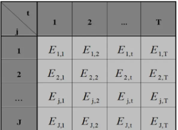
Ej;t=
8 > < > :
product quantity of product j in period t, if item j is produced in period t 0; otherwise
First, the initial solution is generated for the incapacitated version of the problem. This solution then becomes feasible using the soothing mechanism, if it violates the capacity constraint. To this end, Wagner-Whitin algorithm is used for each product. The algorithm is rst applied to items with indepen-dent demand dj;t. It is then applied to each item,
j 2 f2; ; Ng, with both independent and dependent demands.
The products should be produced during the studied period according to the encoding scheme with the following conditions. Let P (j) be a set including all products that can be produced, i.e., there is suf-cient amount of its prerequisites. The sequence can be determined considering the following rules among those products which have necessary conditions for production. In each step, the products in which the examined machine is one of the production process steps are selected. At the initial steps of produc-tion, if a given product has any prerequisite, then a required amount of necessary materials should be available in order to make sure that the product is considered as a candidate for the operation. Also, if the examined machine is in any step except the rst one, then the operation on the product should be completed in previous steps. According to [2], the products in lower levels of General Product Structure (GPS) have greater numbers of demands; also, there are many products which are dependent on these products for the initiation of their production process; therefore, they are assigned higher priority for produc-tion.
If there is more than one output from the previous level, the high-priority product is the one with lower av-erage set-up cost. The avav-erage set-up cost for product j on machine m is derived from Sj;m =
P
iSij;m
P
jPiSij;m.
If the examined product is the rst produced product of the considered machine during the current macro-period, its set-up could be performed in the previous period(s) by considering cost and source. In this case, the carryover option for set-up should be applied to the next period.
A well-known property, called zero-switch prop-erty [31], for the incapacitated lot-sizing problem can be dened as follows: There is an optimal solution to the incapacitated lot-sizing problem (the GCLSP problem without resource constraints), which can be written as:
Product quantity (j; t)Inventory (j; t 1) = 0; or:
0 @XM
m=1 3N
X
f=1
yj;m;f;t
1
A :Ij;t= 0;
or 0 @XM
m=1 3
X
f=1
Nqj;m;f;t
1
A :Ij;t= 0:
Using this property, the production quantity of each item in its production periods can be calculated:
- Step 1: For any item j and period t, if Ej;t = 0,
then set Product quantity(j,t) = 0;
- Step 2: For any item j and any periods t1< t2 T ,
if Ej;t1= Ej;t2= 1 and Ej;t= 0 for all t1 < t < t2,
then:
Product quantity (j; t1)= t2 1X
t=1
0 @dj;t+
X
i2S(j)
aji:di;t
1 A :
(25) In other words, if a product is produced in a given period, the demand of that period as well as those of all periods up to the next production period of that item should be satised. Since no backlogging is assumed, all items are produced in the rst period, i.e.:
Ej;1= 1; 8j = 1; ; N:
In CLSP, the optimal solution may not include zero-switch property, since it also depends on the available capacity of machines. Hence, the solution derived from this property is used as a basic solution to generate a feasible solution considering capacity constraints. This procedure is carried out using the heuristic explained in the next subsection.
3.2. Smoothing mechanism
The initial solution (P1) may be infeasible due to vio-lating capacity constraint. In this case, the smoothing mechanism aims to generate a feasible solution named P2 through shifting products from an infeasible period to other periods. Note that a period is infeasible if the capacity constraint is violated.
In an infeasible period t, a portion of product quantity, named qit, out of total production quantity
of item j in period t is transferred to another period tl.
For each item j produced in an infeasible period t, two quantities are considered to shift to period tl:
Wj;tl: The maximum production quantity of
product j in period t, which guarantees that inventory constraints are still satised. This amount depends on whether tl> t or tl< t;
Qj;t: The quantity of product j in infeasible
period t, which eliminates the resource overload (machine capacity) m in period t by shifting this quantity to another one; Qj;t is calculated by
Eq. (26) as shown in Box I.
In Eq. (26), the comparison is made only for positive values. Note that the amount of Qi;t indicates
that overuse of resource k in period t can be reduced to zero if there is a quantity less than Wi;tl;. The
smoothing mechanism includes the following two steps. 3.2.1. Backward shifts
In this mechanism, the production shifting from each period to earlier periods is analyzed. The procedure starts from the last period and continues toward the rst period. If the period is infeasible, a portion of the selected produced product is moved to earlier periods so that period t becomes feasible. It should be pointed out that the production shifting process is checked for all earlier periods and the best one is selected. The product is also selected by the ratio test, which will be discussed later. If no feasible solution is found by shifting the rst selected product, the procedure applies to the next product. For an infeasible period t, a quantity, Qj;t, out of the entire production amount of
product j in period t is shifted to earlier target period tl, where tl t 1. Note that we have:
= maxf1; the last period among periods prior to period t in which component j is producedg:
The production shifting increases the product stock in a period. In order to meet the inventory balance constraints, the portion of the shifting must be held:
qj;t Wj;tl= min
8 <
: i2P (j)min =tl;tl+1;t 1
fIi;=aijg;
Product Quantity(j; t) 9 =
;: (27) It is noteworthy to indicate that there always exists a component r whose entire production can be moved to an earlier period, r = maxfjjProduct Quantity(j; t) > 0g, since ProductQuantity(i;t)= 0, for all i 2 P (r), where P (r) is
the set of all immediate predecessors of component r. In other words, the entire product of an item can be moved from the current period to earlier periods when none of its components is produced in the current period.
Qj;t= maxm
8 < :
0 @X3N
f=1
bj;m:qj;m;f;t+ N
X
i=1 3N
X
f=1
wij;m:xij;m;f;t+ 3N
X
f=1
bj;m:qj;m;f;t Cm;t
1 A
, pj;m;t
9 =
; : (26)
Box I
The selection of quantity, component, and target period (qj;t; j; tl) is based on the ratio test derived
from cost variation calculation and resource usage. If the procedure continues to the rst period and no feasible solution is found, the forward shifting is applied. Otherwise, procedure P2 terminates.
3.2.2. Forward shifts
This mechanism deals with the production shifting from a given period to later periods. It starts from the rst period to the last one and intends to shift a portion of a product to subsequent periods so as to make it feasible. Similar to the backward shift, the production shift to all earlier periods is checked and the best one is selected. The products are selected one by one and the procedure applies to the next product if no feasible solution is found.
For an infeasible period t, a quantity qj;t out of
the entire production amount of product j in period t is shifted to later target period tl, where t+1 tl and = minfT; the rst period among periods subsequent to period t in which component j is producedg.
Similar to backward shifts, the selection of quan-tity, moved component, and target period is based on the ratio test. The production shift to the next periods reduces the inventory from period t to tl 1; therefore, the inventory balance should be guaranteed. Eq. (25) is used to determine the shifted quantity to the next periods.
qj;t Wj;tl==t;t+1;tl 1min fIj;g: (28)
After shifting, if a feasible solution is found, P2 terminates; otherwise, the backward shift procedure should be applied again.
3.2.3. Ratio test
This procedure aims at selecting the shifted quantity, component, and target period (qj;t, j, tl), i.e., the
quantity qj;t out of the entire production amount of
component j in period t should be moved to an earlier or later target period tl. The values of (qj;t, j, tl)
are chosen so that the following ratio (Eq. (29)) is minimized.
Ratio = Extra cost + :PenaltyExcess decrease : (29) The Extra Cost (Eq. (30)) is calculated as follows:
Extra cost = Additional costTotal cost : (30) By shifting qj;t from period t to tl, the cost variation
calculated by Additional Cost (Eq. (31)) is imposed. Additional cost = qj;t:
"
(cj;tl cj;t)
+Z: 0 @X
k
0 @hj;k
X
i2P (j)
aij:hi;k
1 A 1 A 3
5+SU1+SU2: (31) The rst term of the right-hand side of Eq. (31) calculates the production cost variation. The second and third terms compute the inventory cost variation and set-up cost variation, respectively. Total Cost is the sum of the current system costs, which is derived from the model objective function. The Additional cost parameters can be expressed as follows.
k = (
tl; tl+1; ; t 1 for tl <t (backward step) t; t+1; ; tl 1 for tl >t (forward step)
) ; Z =
(
1; for the backward step 1; for the forward step
) ; SU1 =
(
sj;tl; if Product Quantity (j; tl) = 0
0; otherwise
) ; SU2 =
(
sj;t; if qj;t=Product Quantity(j; tl)
0; otherwise
) : When qj;t is replaced from period t to tl, resource
consumption is changed. Eq. (32) calculates this change as shown in Box II.
In fact, this equation illustrates the overuse ra-tio of resources in period t. In this equara-tion, the resources (machines) whose current demand is more than the available capacity (i.e., the ones with a positive numerator) are calculated. The penalty term in the mentioned ratio represents the resource usage variations caused by the moved quantity qj;t from
period t to tl and is dened by Eq. (33). Penalty = Excess after(t) + [Excess after(tl)
Excess(t) =
M
X
m=1
0 @
0 @X3N
f=1
bj;m:qj;m;f;t+ N
X
i=1 3N
X
f=1
wij;m:xij;m;f;t+ 3N
X
f=1
bj;m:qj;m;f;t Cm;t
1 A
, Cm;t
1
A : (32)
Box II
where:
Excess after(t) = Excess(t) after the move; Excess before(t) = Excess(t) before the move: Note that the penalty cannot be negative and it can be interpreted as a cost for overuse of resources in periods t and tl.
Excess decrease in Eq. (29) is the dierence between Excess after(t) and Excess before(t).
Let a cycle denote a sequence of a backward step and a forward step in the smoothing procedure. In the rst cycle set, = 1. If a feasible solution is not found, the second iteration starts with = 2 and continues up to = n. The more the value of in each iteration, the greater the importance of the use of additional resources.
The number of iterations in this procedure is dened in advance, equal to the number of products. The reason for this can be explained with an exam-ple. Consider a multi-product problem with a two-period time horizon. The production starts from the rst period. Due to the capacity constraint, all the demanded products should be produced in the rst period and some should be transferred to the next period. Although there is a similar algorithm in the literature [30], it uses only backward shift and fails to use the penalty concept for replacement.
3.3. Improvement mechanism
This mechanism starts from a feasible solution gener-ated by the smoothing mechanism and improves it by shifting production from one period to other (either earlier or later) periods. It is obvious that only the improving shifting is accepted. For each period t, a quantity, qj;t, of each component, j, is shifted to a
target period, tl, such that tl < t in the backward step and tl > t in the forward step. For each item i and each target period tl, two quantities in period t are exam-ined: qj;t= Wj;t; qj;t is sampled based on the uniform
distribution U[0; wi;tl]. One reason for selection of the
second random value is that dierent solutions may be obtained with the same initial point. Moreover, the costs vary over time and shifting a quantity qjt< wi;tl
may result in a lower cost. Any candidate set (q; i; tl) in period t among all candidates which minimizes the extra cost is chosen. The procedure terminates when no feasible and improving solution is found.
3.4. Merging procedure
The purpose of this procedure is to further diversify the search. In this procedure, the entire production of an item, j, in a given period is moved to another (either earlier or later) period, tl, in which that item is produced. The aim of production lots merging is to reduce the set-up and production costs. The item production process can be shifted to period tl if this item's lot in the current period is equal to Wj;tl, which is calculated by Eq. (27) for tl < t and
by Eq. (28) for tl > t. If the obtained solution is feasible, the improvement procedure (P3) is applied to enhance the quality of the solution. Otherwise, the obtained solution is used as a new starting point for the Smoothing procedure (P2).
In the rest of this section, an example is provided so as to clarify the proposed heuristic steps.
Assume a problem with N = 4, M = 1, and T = 4, and except for parameters a and D, the values of other parameters are similar to those in Section 3. For this aim, the implementation of the Heuristic's steps is shown in Algorithm 1.
a4;2= 2; a4;3= 3; a2;1= 3; a3;1= 1;
D = 2 6 6 4
15 20 20 10 50 46 48 51 40 45 53 42 80 59 66 71 3 7 7 5 :
The algorithm terminates when maximum iter-ation number (MaxIT) or Max Run Time is reached. The selection of the optimum level for the max iteration of the algorithm is a serious challenge. In this regard, three levels of the mentioned parameters are dened as 15, 20, and 25.
For calibration of the algorithm, several problems are generated and solved; ultimately, 20 is selected as the optimum level of max iteration. Also, Max Run Time is set to 10,000 seconds.
4. The heuristic evaluation
In this section, the performance of the adapted LB and the proposed algorithm is evaluated. To this end, the adapted LB is compared with the optimum solution in very small sized problems. Also, the proposed algorithm is compared with other algorithms.
Algorithm 1. Implementation steps of shifting-based heuristic. is implemented in MATLAB 2011a. All the
experi-ments are run on a PC with a 3.4 GHz Intelr CoreTM
2 Duo processor and 4 GB RAM memory.
4.1. Evaluation of the model and lower bound In order to ensure the accuracy of the LB, a set of 15 instances similar to those used in Mohammadi et al. [13] are generated as follows:
bj;m; ~bj;m U(1:5; 2); dj;m U(0; 180);
hj;m U(0:2; 0:4); pj;m;t U(1:5; 2);
wij;m) U(35; 70); sij;m U(35; 70);
ajijj i U(1; 3):
The capacity of each machine at each period denoted by Cm;t is calculated so as to satisfy the
demand of that period according to the lot-for-lot (L4L) scenarios.
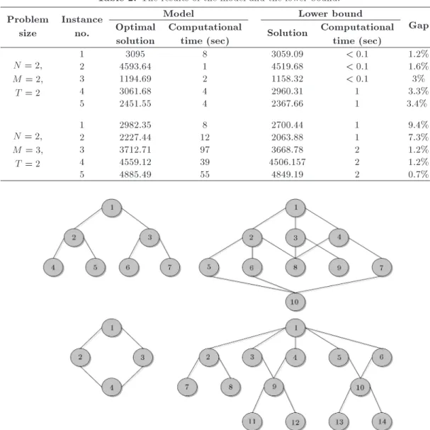
Table 2 shows the results of all instances belonging to the problem with [N = 2; M = 2; T = 2] and [N = 2; M = 3; T = 2]. In Table 2, the rst row shows the optimal solutions while the second row indicates the dierence between the LB and the optimal solution. Also, the computational times in seconds are shown in the third row.
Table 2. The results of the model and the lower bound. Problem
size
Instance no.
Model Lower bound
Gap Optimal
solution
Computational
time (sec) Solution
Computational time (sec) N = 2,
M = 2, T = 2
1 3095 8 3059.09 < 0:1 1.2%
2 4593.64 1 4519.68 < 0:1 1.6%
3 1194.69 2 1158.32 < 0:1 3%
4 3061.68 4 2960.31 1 3.3%
5 2451.55 4 2367.66 1 3.4%
N = 2, M = 3, T = 2
1 2982.35 8 2700.44 1 9.4%
2 2227.44 12 2063.88 1 7.3%
3 3712.71 97 3668.78 2 1.2%
4 4559.12 39 4506.157 2 1.2%
5 4885.49 55 4849.19 2 0.7%
Figure 5. The general product structure for N = 4, N = 7, N = 10, N = 14. The following performance measure (Eq. (34))
shows the gap, i.e., the dierence between LB and the optimal solution:
5
X
i=1
LBsolution;i GOsolution;i
GOsolution;i 100 5; (34)
where LBsolution;i is the solution obtained by the LB
and GOsolution;iis the global optimum for any instance.
The computational times for a problem with [N = 2; M = 2; T = 2] and [N = 2; M = 3; T = 2] are 5.2 and 42.2 seconds, respectively. It reveals that the average computational time grows more than 8 times by adding only one machine to the system.
4.2. Heuristic evaluation
This subsection evaluates the performance of the pre-sented heuristic. To do so, the outputs of the applied algorithms for similar problems with the developed
heuristic in this paper are compared. A set of 15 prob-lems with dierent sizes from (N M T ) = (3 3 3) to (14 14 14) are generated. The used GPSs in the paper are shown in Figure 5. The test instances are taken from the literature [32,33].
These data sets can be divided into three groups:
1. Small-size, including instances with sizes of 3.3.3 to 4.5.4;
2. Medium-size, including instances with sizes of 7.5.5 to 7.7.7;
3. Large-size, including instances with sizes of 10.7.7 to 14.14.14.
Also Cm;tis calculated so that the demand of each
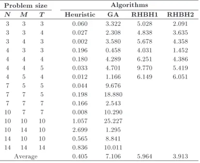
period according to the L4L scenarios is met [34]. Table 3 shows the experimental results in which any instance is solved 5 times and its results are nor-malized through using Relative Percentage Deviation
Table 3. Average Relative Percentage Deviation (RPD) for the algorithms grouped by N, M, T .
Problem size Algorithms
N M T Heuristic GA RHBH1 RHBH2
3 3 3 0.060 3.322 5.028 2.091
3 3 4 0.027 2.308 4.838 3.635
3 4 3 0.002 3.580 5.678 4.358
4 3 3 0.196 0.458 4.031 1.452
4 4 4 0.180 4.289 6.251 4.386
4 4 5 0.033 4.701 9.770 5.419
4 5 4 0.012 1.166 6.149 6.051
7 5 5 0.044 9.676
7 7 5 0.198 18.880
7 7 7 0.166 2.543
10 7 7 0.008 10.290
10 10 10 1.057 25.227
10 14 10 2.699 1.295
14 10 10 0.565 8.841
14 14 14 0.836 10.011
Average 0.405 7.106 5.964 3.913
(RPD) metric calculated as follows (Eq. (35)): RP Di;j =xi;jx xmin;j
min;j :100; (35)
where RP Di;j is the relative percentage deviation of
the jth instance of the ith trial. Also, xi;j is the
objective function value obtained from the jth instance of the ith trial and xmin;j is a minimum value of the
objective function obtained for the jth instance. The average values of RPDs are shown in Table 3. In small instances, all of the algorithms can solve the model, but the results show that the proposed algorithm has a better performance than others with an average RPD of 0.073%. In the medium- and large-scale instances, only GA and the proposed algorithm can solve the problems. In the medium-scale problems, the average RPD of our algorithm, i.e., 0.136%, is much lower than that of GA, i.e., 10.366%. Also, in the large-scale problems, the average RPD of the proposed algorithm is 1.033%, while average RPD of GA is 11.133%, which shows the superiority of the proposed algorithm. Generally speaking, one can say that the proposed algorithm outperforms GA in all categories of instances, i.e., small-, medium-, and large-scale ones, with the average RPD of 0.405% versus 7.106%.
Moreover, in order to further analyze the results, analysis of variance (ANOVA) technique is employed. By using ANOVA, we can study three hypotheses: normality, homogeneity of variance, and independence of residuals. By doing so, we can make sure of the validity of the experiments. The mean plot and Least Signicant Dierence (LSD) interval at the 95% condence level for the dierent algorithms are shown in Figure 6. As can be seen, the proposed algorithm shows better statistical indices than the others.
Figure 6. Mean plot and LSD interval (at the 95% condence level) for the factors of the type of algorithm.
Figure 7. Means plot for the interaction between the type of the algorithms and the number of jobs.
In order to evaluate the robustness of the algo-rithm in dierent situations, possible inuence of the number of products is studied. To show the mutual impact between solution procedure factors and the number of products, the mean plot diagram is depicted (see Figure 7). It is clear that by increasing the number
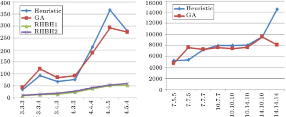
Figure 8. CPU time evaluation of the proposed heuristic against similar algorithms in the literature. of products, the dierence between the performances
of the proposed algorithm and the other algorithms increases signicantly. The previous comparison also shows superiority of the proposed algorithm over the other three ones.
Figure 8 shows the run time comparison of the proposed algorithm with the others with dierent problem sizes.
5. Conclusions and future research directions This paper dealt with the problem of capacitated lot-sizing and scheduling in job shops with carryover set-up and General Product Structure (GPS). An ecient Mixed Integer Linear Programming (MILP) model was rst proposed to formulate the problem. Then, an available Lower Bound (LB) in the literature was adapted to the problem in hand. Due to the complexity of the studied problem, heuristics based on the production shifting concept was also proposed.
The numerical experiments were used to evaluate the proposed model and algorithm. The results indi-cated that the model and the solution method together provided good results for use by a production manager. One opportunity for future research is developing heuristic and meta-heuristic algorithms for the studied problem. Also, using the multi-objective optimization approach can be taken into consideration for further studies.
References
1. Guimar~aes, L., Klabjan, D., and Almada-Lobo, B. \Modelling lotsizing and scheduling problems with sequence dependent set-ups", European Journal of Operational Research, 239(3), pp. 644-662 (2014).
2. Fandel, G. and Stammen-Hegene, C. \Simultaneous lot sizing and scheduling for product multi-level production", International Journal of Production Economic, 104(2), pp. 308-316 (2006).
3. Meyr, H. \Simultaneous lotsizing and scheduling by combining local search with dual reoptimization",
European Journal of Operation Research, 120(2), pp. 311-326 (2000).
4. Karimi, B., Fatemi-Ghomi, S.M.T., and Wilson, J. \The capacitated lot sizing problem: a review of models and algorithms", Omega, 31, pp. 365-378 (2003).
5. Ouenniche, J. and Bertrand, J.W.M. \The nite horizon economic lot sizing problem in job shops: the multiple cycle approach", International Journal of Production Economics, 74, pp. 49-61 (2001).
6. Ouenniche, J., Boctor, F.F., and Martel, A. \The impact of sequencing decisions on multi-item lot sizing and scheduling in ow shops", International Journal of Production Research, 10, pp. 2253-2270 (1999).
7. Maravelias, C.T. and Sung, C. \Integration of produc-tion planning and scheduling: Overview, challenges and opportunities", Computers and Chemical Engi-neering, 33, pp. 1919-1930 (2009).
8. Karimi-Nasab, M. and Seyedhoseini, S.M. \Multi-level lot sizing and job shop scheduling with compressible process times: A cutting plan approach", European Journal of Operational Research, 231(3), pp. 598-616 (2013).
9. Stadtler, H. and Sahling, F. \A lot-sizing and schedul-ing model for multi-stage ow lines with zero lead times", European Journal of Operational Research, 225, pp. 404-419 (2013).
10. Babaei, M., Mohammadi, M., and Fatemi-Ghomi, S.M.T. \Lot sizing and scheduling in ow shop with sequence-dependent set-ups and backlogging", Inter-national Journal of Computer Applications, 8, pp. 0975-8887 (2011).
11. Mohammadi, M., Fatemi-Ghomi, S.M.T., Karimi, B., and Torabi, S.A. \MIP-based heuristics for lotsizing in capacitated pure ow shop with sequence-dependent set-ups", International Journal of Production Re-search, 10, pp. 2957-2973 (2010).
12. Clark, A.R. and Clark, S.J. \Rolling-horizon lot-sizing when set-up times are sequence-dependent", Interna-tional Journal Production Research, 38(10), pp. 2287-2308 (2000).
13. Mohammadi, M., Fatemi-Ghomi, S.M.T., Karimi, B., and Torabi, S.A. \Rolling-horizon and x-and-relax
heuristics for the multi-product multi-level capacitated lot sizing problem with sequence-dependent set-ups", J. Int. Manuf., 21, pp. 501-510 (2010).
14. Mohammadi, M., Fatemi-Ghomi, S.M.T., and Jafari, J. \A genetic algorithm for simultaneous lotsizing and sequencing of the permutation ow shops with sequence-dependent set-ups", International Journal of Computer Integrated Manufacturing, 1, pp. 87-93 (2011).
15. Mohammadi, M., Fatemi-Ghomi, S.M.T., Karimi, B., and Torabi, S.A. \MIP-based heuristics for lotsizing in capacitated pure ow shop with sequence-dependent set-ups", International Journal of Production Re-search, 10, pp. 2957-2973 (2010).
16. Mohammadi, M. and Jafari, N. \A new mathematical model for integrating lot sizing, loading, and schedul-ing decisions in exible ow shops", International Journal of Advanced Manufacturing Technology, 55, pp. 709-721 (2011).
17. Ramezanian, R., Saidi-Mehrabad, M., and Teimoury, E. \A mathematical model for integrating lot-sizing and scheduling problem in capacitated ow shop envi-ronments", International Journal of Advanced Manu-facturing Technology, pp. 347-361 (2013).
18. Ramezanian, R. and Saidi-Mehrabad, M. \Hybrid sim-ulated annealing and MIP-based heuristics for stochas-tic lot-sizing and scheduling problem in capacitated multi-stage production system", Applied Mathematical Modelling, 37(7), pp. 5134-5147 (2012).
19. Lasserre, J.B. \An integrated model for job-shop plan-ning and scheduling", Management Science, 38(8), pp. 1201-1211 (1992).
20. Dauzere-Peres, S. and Lasserre, J.B. \Integration of lot sizing and scheduling decisions in a job-shop", European Journal of Operational Research, 75, pp. 413-426 (1994).
21. Lalitha, J.L., Mohan, N., and Pillai, V.M. \Lot stream-ing in [N 1](1) + N(m) hybrid ow shop", Journal of Manufacturing Systems, 44, pp. 12-21 (2017).
22. Giglio, D., Paolucci, M., and Roshani, A. \Integrated lot sizing and energy-ecient job shop scheduling problem in manufacturing/remanufacturing systems", Journal of Cleaner Production, 148, pp. 624-641 (2017).
23. Wolosewicza, C., Dauzere-Peresa, S., and Aggouneb, R. \A Lagrangian heuristic for an integrated lot-sizing and xed scheduling problem", European Journal of Operational Research, 000, pp. 1-10 (2015).
24. Karimi-Nasab, M., Modarres, M., and Seyedhoseini, S.M. \A self-adaptive PSO for joint lot sizing and job shop scheduling with compressible process times", Applied Soft Computing, 27, pp. 137-147 (2015).
25. Karimi-Nasab, M., Modarres, M., and Seyedhoseini, S.M. \Lot sizing and job shop scheduling with com-pressible process times: A cut and branch approach", Computer and Industrial Engineering, 85, pp. 196-205 (2015).
26. Urrutia, E.D.G., Aggoune, R., and Dauzere-Peres, S. \Solving the integrated lot-sizing and job-shop scheduling problem", International Journal of Pro-duction Research, 52(17), pp. 5236-5254 (2014). DOI: 10.1080/00207543.2014.902156
27. Mateus, G.R., Ravetti, M.G., de Souza, M.C., and Valeriano, T.M. \Capacitated lot sizing and sequence dependent set-up scheduling: an iterative approach for integration", Journal of Scheduling, 13, pp. 245-259 (2010). DOI 10.1007/s10951-009-0156-2
28. Zhang, X.D. and Yan, H.S. \Integrated optimization of production planning and scheduling for a kind of job-shop", International Journal of Advanced Man-ufacturing Technology, 26, pp. 876-886 (2005). DOI 10.1007/s00170-003-2042-y
29. Ouenniche, J. and Boctor, F. \Sequencing. Lot sizing and scheduling of several products in job shop: the common cycle approach", International Journal of Production Research, 36(4), pp. 1125-1140 (1998).
30. Shim, I.S., Kim, H.C., Doh, H.H., and Lee, D.H. \A two-stage heuristic for single machine capacitated lot-sizing and scheduling with sequence-dependent set-up costs", Computers & Industrial Engineering, 61, pp. 920-929 (2011).
31. Afentakis, P. and Gavish, P. \Optimal lot-sizing al-gorithms for complex product structures", Operation Research, 34, pp. 237-249 (1986).
32. Franca, P.M., Armentano, V., Berretta, R.E., and Clarc, A.R. \A heuristic method for lot-sizing in multi-stage systems", Computers and Operations Research, 24(9), pp. 861-874 (1997).
33. Xie, J. and Dong, J. \Heuristic genetic algorithms for general capacitated lot-sizing problem", Computer and Mathematics with Applications, pp. 44263-44276 (2001).
34. Mohammadi, M. and Poursabzi, O. \A rolling horizon-based heuristic to solve a multi-level general lot siz-ing and schedulsiz-ing problem with multiple machines (MLGLSP MM) in job shop manufacturing system", Uncertain Supply Chain Management, 2, pp. 167-178 (2014).
Biographies
Omid Poursabzi a PhD Candidate in Industrial Engineering at Kharazmi University, Tehran, Iran. He received his MS from Kharazmi University in 2013 and BS from Kurdistan University of Science and Technology, Sanandaj, Iran, in 2010, both in Industrial Engineering. His research interests include production planning, econometrics and supply chains, stochastic process, and programming.
Mohammad Mohammadi is an Associate Profes-sor in the Department of Industrial Engineering at Kharazmi University, Tehran, Iran. He received his BS degree from Iran University of Science and Technology,
Tehran, Iran, in 2000, and his MS and PhD degrees from Amirkabir University of Technology, Tehran, Iran, in 2002 and 2009, respectively, all in Industrial Engi-neering. His research and teaching interests include applied operations research, sequencing and schedul-ing, production plannschedul-ing, time series, meta-heuristics, and supply chains.
Bahman Naderi is an Associate Professor of
Indus-trial Engineering at Kharazmi University, Tehran, Iran. He received his PhD in Industrial Engineering from Amirkabir University of Technology, Tehran, Iran, in 2009. He was also with the Applied Optimisation Systems Group at Polytechnic University of Valencia, Spain, as a visiting PhD student in the spring semester of 2008-2009. His research and teaching interests in-clude production scheduling, mathematical modelling, and solution algorithms.
![Table 2 shows the results of all instances belonging to the problem with [N = 2; M = 2; T = 2] and [N = 2; M = 3; T = 2]](https://thumb-us.123doks.com/thumbv2/123dok_us/8372448.2223715/13.892.93.818.163.869/table-shows-results-instances-belonging-problem-n-m.webp)