2.3.1 Future Regulations...8
2.3.2 Correlations...9
2.3.3 Predictive Equations/Models...10
3.0 Experimental Methods...15
3.1 Overview...15
3.2 Description of Utilities Surveyed...15
3.2.1 OWASA...15
3.2.2 Burlington...18
3.2.3 Durham...19
3.2.4 Raleigh...20
3.2.5 High Point...20
3.2.6 Winston-Salem...21
3.3 Sampling and Handling Procedures...22
3.3.1 Glassware Preparation...22
3.3.2 Sample Collection...22
3.3.3 TOC Analysis... ...23
3.3.4 TOX Analysis...24
3.3.5 DBP Analysis...25
4.0 Experimental Results...27
4.1 OWASA...27
4.2 Burlington...31
4.3 Durham...31
4.4 Raleigh...38
4.5 High Point...42
4.6 Winston-Salem...42
4.7 Summary...49
5.0 Description of Disinfection By-Product Predictive Model...52
5.1 Introduction...52
5.2 Predictive Equations...52
5.2.1 DBP Equations...52
5.2.2 Chlorine Decay Equations...55
5.2.3 Equation Inputs and Their Sources...57
5.2.3.1 TOC and UV-254...57
5.2.3.2 Chlorine...57
5.2.3.3 Temperature and pH...58
5.2.3.4 Residence Times...58
5.2.3.5 Bromide and Ammonia...60
5.3 Chlorine Dose Method...63
5.3.1 One Point of Chlorination...64
5.3.2 Two Points of Chlorination...67
5.4 Chlorine Residual Method...69
6.2 One Point of Chlorination...74
6.3 Two Points of Chlorination...91
6.4 Summary...94
6.5 Shortcomings of the Model...97
7.0 Conclusions and Recommendations...99
References...102
Appendices...106
Appendix A: Sample Collection Flowsheets for Each City
Appendix B: Boundaries for the Predictive Equations
Appendix C: Calculation of Residence Times Used in Model
Appendix D: Modeling Results: Second and Third Sample Days of Each City
Appendix E: Cumulative and Relative Frequency of Predicted DBP
5.4 Chlorine Dose Method - Two Points of Chlorination, Raw and Filtered...68
5.5 Chlorine Dose Method - Calculation of DBP Formation For Two Points of
Chlorination, Raw and Filtered...70
5.6 Chlorine Dose Method - Two Points of Chlorination, Setded and Filtered...71
6.1 Predicted vs. Observed Chlorine Residual at OWASA - 8/27/91...84
6.2 TTHM - Cumulative Frequency vs. Deviation...95
6.3 TTHM - Relative Frequency vs. Deviation...95
A. 1-A. 13 Plant Flowsheets for Each Sampling Day
4.1-4.6 OWASA-Results of Survey...28
4.7-4.12 Burlington-Results of Survey...'...32
4.13-4.18 Durham-Results of Survey...35
4.19-4.24 Raleigh - Results of Survey...39
4.25-4.30 High Point - Results of Survey...43
4.31-4.36 Winston-Salem-Results of Survey...46
4.37 Average DBP Concentrations and Relationships in the Distribution System...51
5.1 Estimated Residence Times...61
6.1 OWASA - Chlorine Dose Method Modeling Results - 8/27/91...75
6.2 Burlington - Chlorine Dose Method Modeling Results - 7/30/91...76
6.3 Effect of Changes in Bromide Concentration on Model Predictions For
OWASA and Burlington...78
6.4 OWASA - Chlorine Residual Method Modeling Results - 8/27/91...79
6.5 Burlington - Chlorine Residual Method Modeling Results - 7/30/91...80
6.6 Chapel Hill-Chlorine Decay Method Modeling Results-8/27/91...81
6.7 Burlington - Chlorine Decay Method Modeling Results - 7/30/91...82
6.8 Durham-Brown WTP-ModeUng Results-6/18/91...86
6.9 Durham-Williams WTP-ModeUng Results-6/18/91...87
6.10 High Point - Modeling Results - 8/2/91...89
6.11 Effect of Changes in Bromide Concentration on Model Predictions For WTPs
Chlorinating Their Water Once...90
6.12 Raleigh-Modeling Results-7/30/91...92
6.13 Raleigh - Modeling Results - 2/3/92...93
6.14 Summary of Modeling Results...96
B.1-B.6 Experimental Limits for DBP Predictive Equations
MBAA Monobromoacetic acid
CHCI3 Chloroform
CHBrCl2 Dichlorobromomethane
CHBr2Cl Dibromochloromethane
MCAA Monochloroacetic acid
DCAA Dichloroacetic acid
TCAA Trichloroacetic acid
CI2 Res. Chlorine Residual
DBP Disinfection By-Product
DS Distribution System
EPA Environmental Protection Agency
f Filtered WaterFW Finished Water
HAAs Haloacetic acids (MCAA, DCAA, TCAA, MBAA)
MCL Maximum Contaminant LevelMG Million Gallons
ND Not Detected
NOM Natural Organic Matter
NORS National Organics Reconnaissance Survey
TOX Total Organic Halide
TTHMs Total Trihalomethanes (sum of CHCI3, CHCl2Br, CHBr2Cl, ug/1)
monitoring programs for these compounds, and has started to set limits on the
concentrations present in finished drinking water.
Trihalomethanes (THMs) are a class of compounds produced from the chlorination of
drinking water and have been regulated at a Maximum Contaminant Level (MCL) of 100
ug/1 (Total Trihalomethanes, TTHM) since 1979. In the near future, the level may be
lowered to either 50 or 25 ug/1 and MCLs may be set for the individual THM species and
for other DBFs, such as the haloacetic acids (HAAs). The promulgation of these limits will
effectively force water treatment utihties to significantiy modify their treatment trains to
achieve compliance. The utilities are presentiy aware of the amount of THM formation in
both the plant and the distribution system. However, determining the process modifications
which will lower DBF formation through pilot-testing can prove costiy and
time-consuming. Pilot-plant testing will likely require more time than the utilities have available
and contracting the work out to consulting firms is a viable, but more expensive alternative.
A cheaper and less time-consuming approach for investigating the effects of alternative
treatment processes on DBF formation is through the use of predictive models. Equations
predicting the formation of DBFs from chlorination have recentiy been developed and are
being incorporated into a water treatment plant model which will predict DBF formation
through a proposed treatment train and into the distribution system. This model is the first
time predictive equations and correlations for water treatment processes have been
utilities treated their water in a conventional fashion consisting of flocculation,
sedimentation, and filtration, and all disinfected using only free chlorine. The objectives of
this project were:
• to evaluate the levels of DBPs (THMs, HAAs) throughout
the treatment plant and distribution system during three
seasons for six utilities;
• to model the formation of these DBPs by three different methods using the predictive equations. One of the three
methods is the procedure developed and used in Malcolm
Pimie's WTP Model (1992); and
• to determine the ability of the model to accurately predict
DBP formation by comparing the model predictions to the concentrations measured.
It should be mentioned that analysis was also performed on the same North Carolina
database and investigated the trends and correlations between DBP formation and water
quality characteristics. The results of this study can be found in the Master's Thesis by Alexa Obolensky titled DBP Formation in North Carolina Drinking Waters: Observations
application of chlorine was yet another step towards making water safer to drink by
reducing the risk of contracting waterbome diseases. Most of the recent waterbome disease
outbreaks have been the result of insufficient addition of chlorine to the water withsubsequent depletion of the residual to zero. Applying enough chlorine for required
disinfection levels is important; without it, diseases from waterbome pathogens would be
epidemic, especially at the pollution levels present in many of our raw water sources today.
The application of chlorine to drinking water has several other purposes in addition to
disinfection. Chlorine is widely used in drinking water treatment to control taste- and
odor-causing organics, to decolorize the water, to oxidize inorganics such as iron and
manganese, and to control the growth of nuisance organisms in the treatment basins. The
decision of how to use chlorine for drinking water treatment can be compUcated because of
these many roles of chlorine.
2.2 Chlorinated Disinfection By-Products
2.2.1 Occurrence of DBFs in Drinking Water
The use of chlorine as a disinfectant has had a positive impact on drinking water quality by
decreasing the incidence of waterbome disease. However, the discovery of chlorinated by¬
products in 1974 (Rook) changed this situation. Rook discovered that the chlorine used for
disinfection reacted with natural organic matter (NOM) present in the water to produce
The discovery by Rook (1974) set off a series of surveys aimed at determining the extent of
occurrence of DBFs in drinking water. The National Organics Reconnaissance Survey (NORS) for Halogenated Organics was conducted by the EPA with this goal in mind
(Symons gt aL, 1975) and examined the THM concentrations in the raw and finished waters of eighty water utilities nationwide. The survey concluded that the application of
chlorine creates organic compounds, most notably THMs, that were not present in the raw water. The median finished water THM concentrations for the eighty utilities were:
chloroform, 21 ug/1; bromodichloromethane, 6 ug/1; dibromochloromethane, 1.2 ug/1.
Bromoform was not detected in the finished waters of two-thirds of the utilities examined.
Furthermore, THM concentrations were shown to increase with the organic content of the water (TOC) and when chlorine was appUed to the raw water instead of to the settled water.
Singer et d. (1981) analyzed THM formation at nine utilities in North Carolina. Aknost all of the utilities surveyed (12 of 13) used conventional surface water treatment and chlorine
as a disinfectant. Samples from each utility were taken during all four seasons in order to
determine the effects of temperature and organic content on THM formation. Similar to the
NORS survey, THM concentrations increased with organic content (raw water), and
decreased by changing the point of chlorine application from the raw to the settled water.
However, the median TTHM concentration in the finished water for all utilities visited was
58 ug/1, slightly higher than the median observed concentration in the NORS survey of 41
ug/1. The average TOC concentration of the North Carolina utilities was 4.4 mg/1, much
higher than the average NORS TOC concentration of 1.5 mg/1. Seasonal and temperature
variations in the formation of THMs were also observed. Much higher THM concentrations were measured during the summer, when the temperature and TOC concentration were
higher, than were measured in the winter, when the temperature and TOC concentration
were lower.
In 1988, a survey funded by the American Water Works Association Research Foundation (AWWARF) was completed (McGuire and Meadow, 1988). Over 900 U.S. utilities were
surveyed, with greater than 80% using chlorine as a disinfectant Utilities serving over
10,000 people responded to a questionnaire addressing existing and previous treatment methods, THM concentrations for the three-year period of 1984 to 1986, and other water
United States and 10 located in California. Finished water concentrations of a wider range of DBFs were measured in this study than in previous studies and included THMs, HAAs, haloacetonitriles, haloketones, and a number of others. The THMs were found to be the largest class of the DBFs measured, on a weight basis, with a median TTHM concentration of 39 ug/1, similar to the NORS and AWWARF surveys. The HAAs were the next largest class and had a median concentration of 19 ug/1 (sum of HAA species). The survey showed that the presence of bromide in the water shifted the distribution of the THMs and HAAs to the more brominated species. The pH was also shown to affect the THM and HAA
concentrations, with higher pHs favoring THM formation and decreasing HAA formation.
2.2.2 Implications
The implications of the discovery of these by-products are still being evaluated. Studies have linked these compounds to cancer. Chloroform has been shown to target the kidney and liver of rats, mice and dogs when administered at relatively high doses, the effects ranging from relatively mild changes in the blood to irreversible cell damage (Orme and Ohanian, 1988). Furthermore, cancer was induced in the kidneys of mice and rats exposed to chloroform in a number of ways, most notably through drinking water. Mice exposed to bromodichloromethane and dibromochloromethane for 14 days showed decreased
functioning in their immune system (Orme and Ohanian, 1988) and, more recentiy, dichloroacetic and trichloroacetic acids have been shown to induce liver cancer in mice
(DeAngelo and McMillan, 1990). Studies examining bladder, colon and rectal cancers in
humans have demonstrated a weak relationship with chloroform (Crump, 1983).
The mutagenicity of these compounds has also been investigated using the Ames Assay
(Ames et aL, 1975). The assay is a simple method for determining the amount of genetic mutation induced in bacteria by specific compounds. While the assay has been used
•
has been questioned (Loper, 1980). Chlorinated drinking water has been found to contain significant levels of mutagenic activity (Schwartz si M», 1979; Maruoka and Yamanaka,
1980; Kronberg £t aL, 1985), with one study showing a greater mutagenic activity present in the treated waters of 14 U.S. utilities when compared to their raw water sources, with the implication that chlorine increases mutagenicity (Glatz si. aL> 1978). Seventy-one
chemicals examined by the Ames test demonstrated that bromodichloromethane,
dibromochloromethane and bromoform were mutagenic while chloroform was not (Loper, 1980). Although the results of these studies are far from conclusive, the EPA has made chlorinated disinfection by-products a high priority on their drinking water regulatory
agenda.
2.2.3 Existing Regulations
Chlorination by-products are a result of water treatment, so it is believed that they can be
controlled. The present regulations, as promulgated by the EPA in 1979, set a Maximum Contaminant Level (MCL) in drinking water of 100 ug/1 for Total THMs. This level is the
sum of the concentrations of chloroform, bromodichloromethane, dibromochloromethane
and bromoform. All utilities servicing more than 10,000 people are required to meet the
MCL. Systems servicing less than 10,000 people are not covered by the MCL; compliance
with the MCL is left to the discretion of the state. The TTHM concentration, for compliance purposes, is computed using a running annual average calculated from quarterly
measurements of four samples per plant taken on the same day (Cotruvo, 1981). Presentiy, there is no MCL for haloacetic acids or any other DBPs, although draft MCLs for selected
HAAs and other DBPs are expected shortly, including more stringent MCLs for the THMs.
2.2.4 Control
The existing regulations changed the manner by which many utilities treat their water. Three options are available for controlling and reducing the amount of DBPs formed:
precursor removal and moving the point of chlorine appUcation; removing the DBPs after they are formed; using alternative preoxidants and disinfectants.
Removing DBP precursors (NOM) before the chlorine is applied to the water would effectively decrease DBP formation. Various techniques are used to remove NOM, the
formation.
The removal of DBFs subsequent to their formation is possible by stripping them from the water using air (effective only for THM removal), adsorption (activated carbon), ion
exchange, and membranes. While not very much is known regarding the removal of DBFs with these technologies, they all have the same potential problems: disposal of the DBFs removed, and expensive operating costs (Weber and Smith, 1986). Regardless of which of
these DBF removal technologies is used, DBFs still continue to form in the distribution system.
A third possibility for controlling chlorinated DBFs is to minimize or eliminate the use of chlorine. The primary goals for applying chlorine at the beginning of the treatment train are
to decolorize the water, oxidize taste- and odor-causing organics, oxidize reduced iron and manganese, and control biological growth in the treatment plant basins, as well as for
disinfection. Moving the application of chlorine further down the treatment train, or totally
eliminating its use, means these responsibilities need to be fulfilled by alternative
chemicals. Common alternatives include potassium permanganate, chlorine dioxide, ozone, various advanced oxidation processes (AOFs), and combined chlorine. A major drawback to many of these alternatives is that littie is known about their by-products, and some of them (e.g. permanganate, combined chlorine) don't have the disinfecting power of free
chlorine.
Combinations of these alternative preoxidants and disinfectants have been shown to substantially decrease the formation of THMs (Myers, 1990). A survey of U.S. water
treatment plants conducted by McGuire and Meadow (1988) showed that to meet the MCL
of 100 ug/1 for TTHMs, 18% of the modifications to treatment were through plants
switching from free chlorine to combined chlorine, while 58% of the modifications were
the more stringent regulations that are being proposed, utilities will need to investigate treatment modifications in much greater detail.
2.3 Predicting Disinfection By-Product Formation
2.3.1 Future Regulations
In 1986, the signing of the Safe Drinking Water Act (SDWA) Amendments into law forced
the EPA to plan a timetable for the regulation of drinking water. As set down by the law,
83 MCLs must be established by the EPA, with 25 new MCLs set every three years after
promulgation of these initial 83. These MCLs are to be met by all pubUc water supplies, including utilities servicing less than 10,000 people (Pontius, 1991). The upcoming Disinfection By-Product rule will partially satisfy these requirements, with a formal proposal of the new rule expected to be ready in June 1993 and final rule promulgation in June 1995. The proposed rule will set MCLs for inorganic disinfection by-products and for organic disinfection by-products, as well as for some disinfectants (Pontius, 1991). The organic by-products to be regulated include the four THM species and the haloacetic acids, with three options being considered for the THMs:
1. one MCL for TTHMs, at a lower level than the present one; 2. separate MCLs for each of the four THM species;
3. an MCL for TTHMs and an MCL for each THM species.
Separate MCLs are being considered for each THM species because their health risks differ greatiy. Similarly, three options are being considered for the haloacetic acids:
1. MCLs for dichloroacetic acid and trichloroacetic acid; 2. an MCL for total haloacetic acids (sum of mono-, di-,
trichloroacetic acid, monobromo- and dibromoacetic acid, and bromochloroacetic acid);
3. a combination of the two previous options.
in the treatment train. However, this approach can be costiy and time-consuming. To help
estimate these concentrations, several correlations using water quality parameters have been developed. For the most part, these correlations have focused on THMs, with some
research investigating the haloacetic acids. Because THMs have been shown to result from the reaction of chlorine with natural organic matter, Total Organic Carbon (TOC) has been closely examined as a surrogate parameter for NOM as DBP precursors. A number of studies have confirmed that there is a strong correlation between the THMs formed and the raw water TOC (Singer, £l aL, 1982; Edzwald, et aL 1985; Singer and Chang, 1989). The use of UV-254 absorbance as a surrogate has also been examined for drinking waters and shows a similarly strong relationship (Singer, el aL. 1982; Edzwald, ££ aL, 1985; Singer and Chang, 1989). A drawback to these correlations is the specificity for each water
studied, making it difficult to use data from one water to predict TEIM formation in another.
An alternative approach for estimating DBP concentrations in drinking water has been investigated by analyzing the treated water for the Total Organic Halide (TOX)
concentration. Strong correlations have been observed between the instantaneous TTHM and TOX concentrations in the distribution systems of numerous utilities (Singer and Chang, 1989; Reckhow and Singer, 1990). In general, the chlorination of drinking water and a variety of fulvic and humic acids has shown chloroform to comprise 20% of the TOX on a chlorine-equivalent basis (Reckhow and Singer, 1990; Reckhow £l aL. 1990). These studies also showed dichloroacetic acid accounting for 6% of the TOX and trichloroacetic acid accounting for 18%, also on a chlorine-equivalent basis.
only the chlorine dose was significant in predicting the chloroform concentration by the
following equation:
CHCI3 = 22.23(Cl2 Dose) - 11.24 (2.1)
The specificity to the utilities studied and the dependence on only one parameter limits the use of this equation. However, a solid relationship between chloroform formation and chlorine dose was established.
2.3.3 Predictive Equations/Models
The development of correlations for predicting THMs and other DBFs is a solid beginning,
but a more thorough approach needs to be examined. Correlations are limited since they
include only one parameter for prediction, while it is well-known that DBF formation is dependent upon a variety of factors including pH, temperature, precursor (TOC)
concentration, contact time and chlorine dose. With this in mind, researchers have
gradually developed kinetic and empirical relationships to try to take this complexity into account. Trussell and Umphres (1978) first introduced a reaction kinetic approach with the
following equation:
^I^ = k(Cl2)(Cr (2.2)
where k is a rate constant, CI2 is the chlorine concentration, C is the concentration of the
organic precursor (TOC), and m is the order of the reaction with respect to the precursor concentration. Applying Equation 2.2 to a Umited database, they found a good fit, with an order of reaction (m) equal to three. However, the values used for k and C were specific for the water examined. It should be mentioned at this point that calibration using a set of data of an equation such as the one above refers to the development of the equation based upon the observations in the data set. Verification of the equation imphes testing the ability to predict the target parameter but with an data set unrelated to the set used to calibrate the
model.
prediction for contact times greater than 1.5 hours, but underestimated TTHM formation for shorter times. These results suggested that the order of the reaction is not constant and
changes with time. It was also noted that the rate constant k^ was dependent on temperature
and pH, increasing as each parameter increased.
Investigation into using a large number of water quality characteristics for the prediction of
THMs was furthered by Engerholm and Amy (1983). Examining the effects of time, pH, TOC concentration, and chlorine dose, the following relationship for chloroform was developed:
Cb Dose
CHCI3 = ki k2(TOC)0-95 (-^^^—)0.28 tz (2.4)
where k^ was pH-dependent and k2 and z were temperature-dependent; all three
parameters were empuically-derived. While this equation predicted chloroform formation based on more parameters than previous equations, the data used in deriving the equation
were from the chlorination of a commercial humic acid and not from natural waters.
A study of the chlorination of nine natural waters by Amy et ^ (1987) is the most
comprehensive database developed to predict THM formation. The waters were collected
from across the U.S. and represented a diverse range of natural water systems. Each water
was examined by subjecting it to a series of experiments covering a range of operating conditions and included varying the following parameters: TOC concentration, UV-254
absorbance, chlorine dose, contact time, temperature, pH, and bromide concenttation (Br).
All of these parameters were measured and over 1000 data points were generated. The data
were used to develop two predictive equations, one using a multiple nonlinear regression
(nonlinear model), and the second using a multiple linear regression with logarithmic
transforms (log model). Preliminary analysis determined that the pH and the bromide
concentration were better represented by pH* = (pH - 2.6) and Br* = (Br +1), because
+ 1) were obtained because most ambient bromide levels are less significant than 1.0 mg/1. After closely examining the data, the following equations were developed:
Nonlinear Model:
Short-Term Equation (t <= 8 hours):
TTHM = -2.46 + 0.315[(TOC)(UV-254)] + 0.184exp[0.0762(T)]
+ 0.00611(Cl2 Dose)l-33 + 0.215(Br)l-51
+ 1.16(t)0-252 + 0.0887(pH - 2.6) (2.5)
Long-Term Equation (t >= 24 hours):
TTHM = -16.9 + 0.849[(TOC)(UV-254)] + 0.407exp[0.0834(T)]
+ 0.00678(Cl2 Dose) 1-59 + 0.772(Br)l-65
+ 9.75(t)0-0707 + o.402(pH - 2.6) (2.6)
Log Model:
TTHM = 0.00309[(TOC)(UV-254)]0-44(Cl2 Dose)0-409(t)0.265(T)1.06
(pH-2.6)0-715(Br+1)0-036 (2.7)
where TTHM is the total trihalomethane concentration (umol/1), TOC, Q2 Dose, and
bromide are in mg/I, UV-254 is the UV absorbance at 254 nm (cm'^), T is the temperature
(^C), and pH is on a scale of 1 through 14. Initial regressions for the nonlinear modelshowed that a single equation significantly underpredicted TTHMs at short contact times and overpredicted TTHMs at long contact times. For this reason, the nonlinear model was divided into two equations, one for predicting the TTHM concentration up to 8 hours and the other for predicting TTHM concentrations after 24 hours. Data were not collected between 8 and 24 hours and so the equations are not valid for TTHM concentrations
•
low TTHM concentrations and overpredict at high TTHM concentrations. These results should be regarded with care, however; in many cases, the external data were extracted from figures in journal articles and was not very accurate.
Similar empirical equations predicting concentrations of the individual THM species (Malcolm Pimie, 1992), tiie individual HAA species (Haas, 1991; JMM, 1992), and die chlorine residual concentrations (Dharmarajah et al., 1991) have been developed using the
same approach as Amy si sL (1987). The equations for the individual THM species were
developed, in fact, from the same database. The full equations are presented and discussed
later, in Chapter 5.
The equations have been incorporated into a model developed by Malcolm Pimie (1992) for the USEPA which simulates DBP formation in water treatment plants. The model has the ability to predict water quality and composition through the treatment train and, to a limited extent, into the distribution system. Predicted water quality characteristics include pH, alkalinity, hardness, TOC, UV-254 absorbance, chlorine residual, and THM and HAA formation. The user chooses the desired treatment train and inputs the raw water
characteristics and the residence times to the model. The model then calculates the water
characteristics through the plant and into the distribution system. By altering the method of treatment, as discussed earlier in this chapter, the user can observe relatively quickly the subsequent effects on finished water quality. Results fk)m the model can be compared with the costs of each treatment modification to provide utilities a quick, inexpensive method for
determining how to achieve compliance effectively.
Burlington; Durham; Raleigh; High Point; and Winston-Salem (see Figure 3.1). All of the utilities used surface waters as their source of supply and chlorine as the primary and secondary disinfectant.
Each utility was sampled three times, at approximately four month intervals. Water samples were collected at the water treatment plants and at several locations in the distribution system. The samples were then transported back to the University of North Carolina at Chapel Hill (UNC-CH) where they were analyzed for total organic carbon (TOC), total organic halogen (TOX), and a selection of disinfection by-products (DBFs) which included trihalomethanes (THMs) and haloacetic acids (HAAs).
The TOC samples were collected from the raw water and the settled water at all of the plants visited. The TOX and DBF samples were collected from the setded water, the finished water and from within the distribution system (see Figure 3.2). The settled water samples were used to determine the background TOX and DBF levels in the water, making it important to collect these samples immediately prior to the point of chlorine application. If the plant was chlorinating its raw water, the background TOX and DBF samples were collected from the raw water instead of the settled water.
3.2 Description of Utilities Surveyed
3.2.1 OWASA
The towns of Chapel Hill and Carrboro are served by one water treatment plant which is operated by the Orange Water And Sewer Authority (OWASA). The plant has a design capacity of 10 MGD and it's sources of water are University Lake and the Cane Creek Reservoir. Most of the time, the plant uses only water from University Lake while
t
NWinston-Satem
OWASA
Durham
Raleigh
High Point
Burlington
^
North Carolina
Chlorine.
RAPID MIX
\
FLOC BASIN
I
SEDIMENTATION
BASIN
4
Settled Sample ^ "lOCTOX, DBFsFILTERS
I
TOX. DBPs, Chlorine Residual
CLEARWELL
I Finished Sample
DISTRIBUTION
SYSTEM
TOX, DBPs, Chlorine Residual
Figure 3.2: Locations for Water Sample Collection
The raw water is pumped directly from the source into the rapid mix basins where alum and potassium permanganate are added. The average alum dosage is about 40 mg/1, dropping the pH to an average of 6.2. From the rapid mix basins the water has two options. It can flow either through a series of flocculation basins and conventional sedimentation basins or through a set of Super Pulsators. Once the water passes through one of the two clarification trains, it is collected in a common channel which leads to the dual media filters. Chlorine is applied on top of the filters at a sufficient level to maintain a residual of about 1.4 mg/1 in the finished water. Following filtration the water flows into a 1.6 MG clearwell before it is pumped into the distribution system. The flowsheet for the plant is shown in Figure A. 1 indicating where samples were collected.
The plant was operating in this same manner on all three sampling days. The plant was using only University Lake as its raw water source on the first and third sampling days, while a mixture of University Lake and Cane Creek water was used on the second day.
3.2.2 Burlington
The city of Burlington is primarily served by the Thomas water treatment plant, although there is a second plant which is operated in times of high demand as well as during some weekends. The plant draws it's raw water from Old City Lake which, on average, has the following water quality: turbidity, 60 NTU; color, 90 CU; pH, 6.6; alkalinity, 25 mg/1 as CaC03; hardness, 30 mg/1 as CaC03.
The raw water is pumped into the plant where an average alum dose of 55 mg/1 is applied before it enters the flash mix basins. After passing through the flocculation and
sedimentation basins, chlorine is added to the water before filtration. The 5.5 MG clearwell
has a theoretical residence time of 9 hours at the average daily flow. Three headers leave the plant, each with the capacity to apply chlorine immediately after the pumps. This second point of chlorine addition is used to boost the residual only when necessary. For this reason, the amount of secondary chlorine applied is relatively small. The total chlorine applied to all three headers averages 0.2 mg/I/day, a negligible amount.
On the second day of sampling, October 25th, 1991, the plant was shut down
3.2.3 Durham
Durham is served by two water treatment plants, the Brown and Williams plants, which have the same raw water source. Lake Michie. The raw waters entering the plants have the same characteristics which are as follows: turbidity, 8 NTU; color, 35 CU; pH, 7.0;
alkalinity, 15 mg/1 as CaC03; hardness, 22 mg/1 as CaC03. The two plants send their
finished water into a composite distribution system, making it difficult to determine which parts of the city are served by which plant. The raw water enters the Brown plant and is dosed with an average of 36 mg/1 of alum. After passing through the rapid mix basins, thecoagulated water flows through the flocculation and sedimentation basins. Chlorine is applied to the water before it passes through the filters. After storage in two 5 MG clearwells, the water is pumped into the distribution system through a 42" header.
The Brown plant was undergoing expansion throughout the time period of this study, and
is now rated at 30 MGD. The new filters were only in service during the third sample day, doubling the theoretical residence time through the filters. On the second and third sample days, the 'settied' samples were taken, respectively, from the top of the filters and from the channel leading from the sedimentation basins to the filters. In both instances, chlorine had already been applied to the water. Figures A.4 and A. 5 show the flowsheets and sample collection points for the Brown plantThe Williams plant has an identical treatment train to the Brown plant and is rated at 22
MGD. The raw water is dosed with an average of 30 mg/1 of alum, which lowers the pH to
6.3. Enough chlorine is applied on top of the filters to maintain a residual of 2.2 mg/1 in the
finished water. The water is stored in three 1 MG clearwells before it is pumped into the
20
3.2.4 Raleigh
The city of Raleigh is served by the 62.5 MGD Johnson water treatment plant. Raleigh alternates applying chlorine at three different points in the treatment process: to the raw water, to the filter influent, to the filter effluent Chlorine is applied at only two points during any given time.
The Johnson plant's raw water source is Falls of the Neuse Lake which, on average, has the following water characteristics: turbidity, 3 NTU; color, 25 CU; pH, 6.6; alkalinity, 30 mg/1 as CaC03; hardness, 30 mg/1 as CaC03. When the plant is prechlorinating, an
average dose of 7.0 mgA of chlorine is applied to the raw water as it enters the rapid mix basins. The water then passes through the flocculation and sedimentation basins which have theoretical residence times, at an average flow of 45 MGD, of 14 minutes and 48 minutes, respectively. After leaving the sedimentation basins, the water flows through the plant's 20 filters, each with a theoretical residence time of 22 minutes. Chlorine is then applied to the filter effluent at an average dose of 1.5 mg/1 before passing through six clearwells (total volume = 12.8 MG) on the way to the distribution system. Figures A.7, A.8 and A.9 are the flowsheets for each sample day, illustrating the multiple locations of chlorine application.
The background water samples collected on the first sampling day were for settled water, after chlorine had been appHed. On the second sampling day, the background samples collected were for raw water, before chlorine had been applied. These raw water samples still contained some chlorine since the plant returns its filter backwash water to the raw water reservoir. On the third sampling day, chlorine was not being applied to the raw water, but instead was being applied to the filter influent. Chlorine was still being appUed to the fiilter effluent, at a dose of 1.3 mg/1.
3.2.5 High Point
The city of High Point is served primarily by one water treatment plant (the Ward WTP). As in Burlington, the second plant (1 MGD) only operates intermittentiy and was not a factor in this study. The Ward plant is rated at 20 MGD, although it rarely exceeds 15
the rapid mix basins, the water travels through the flocculation and sedimentation basins, at
which point chlorine is applied before the filters at an average dose of 5.0 mg/1. From the
filters, the water passes through the clearwell (225,000 gallons), from which it is pumped
into the finished water reservoir (5 MG). Water samples were collected from the same locations on each sample day.
Figure A. 10 shows the plant flowsheet and locations of sample collection for all of the
sampling days.
3.2.6 Winston-Salem
Winston-Salem is served by the Thomas (24 MGD) and Neilson (48 MGD) water treatment plants. The raw water source for the Thomas plant is a fifty-fifty blend of the Yadkin River and Salem Lake, while the Neilson plant uses only the Yadkin River as its source. On average, the turbidity of the Yadkin River is 20 NTU, while that of Salem Lake is 12 NTU.
Otherwise, the two source waters have the same average pH (7.0), alkalinity (20 mg/1 as
-CaC03), and hardness (20 mg/1 as CaC03).
The raw water enters the Thomas plant where it is dosed with alum (16 mg/1) and chlorine
(3.0 mg/1) before the rapid mix basins. Flowing through the rapid mix, flocculation and
sedimentation basins, the filters, and three clearwells (total volume = 6 MG), chlorine (1.2
mg/1) is again applied to the water as it enters the distribution system. The theoretical
residence time between the two points of chlorine appUcation is 14 hours at an average flow
of 18 MGD. The treatment train of the Thomas plant for all three sample days is shown in
FigureA.il.
The Neilson plant has an identical treatment train. Alum is applied to the raw water as it
enters the plant, with an average dose of 18 mg/1. On the first sampling day, chlorine was being applied to both the raw water and the filter effluent The theoretical residence time between the two points of chlorine application is 6.5 hours at the normal operating flow of 26 MGD. On the second and third sampUng days, chlorine was being applied to both the
system via four headers. Figures A. 12 and A. 13 show the plant flowsheet and the locations of sample collection for each sampling day.
The plants are located in the eastern (Thomas) and westem (Neilson) regions of the city, making the task of determining which plant serves each distribution point relatively easy.
3.3 Sampling and Handling Procedures
3.3.1 Glassware Preparation
The water samples were collected in 40-ml Pierce vials with screw-on caps containing Teflon-lined septa (Pierce Chemical Co., Rockford, DL). Prior to sample collection, the
vials were soaked in chromic acid (Fisher Scientific Co., Fair Lawn, NJ) for 30 minutes,
rinsed thoroughly with deionized, distilled water, and dried in the oven overnight at 1(X) OC. The caps and septa were soaked in detergent, rinsed in deionized, distilled water, and dried in the oven overnight at 80 ^C. The vials were assembled and stored capped until use. The day before sampling, the vials were labeled with the date, location, and the
parameter to be analyzed.
3.3.2 Sample Collection
The water samples collected at the treatment plants were usually taken from the sample taps in the plant laboratory. When this was not possible, the samples were collected from the appropriate basin or pipe in the treatment train. The samples collected in the distribution system were drawn from a sink in the men's restroom of the sample site. Before collecting samples from the sink, the tap was checked for an aerator and removed if present. The tap
was then turned on and the water was allowed to run for two to three minutes before
samples were collected.
The sample vials were filled with a minimum of turbulence at which time the appropriate quenching and preserving agents were added to the vials:
- TOC samples: phosphoric acid * - TOX samples: phosphoric acid *
and Total Chlorine Test Kit, Model CN-70 (Hach Co., Loveland, CO). The analysis is based on Method 4500-Cl G, DPD Colorimetric Method (Standard Methods, 1989). The
chlorine residual of Chapel Hill tap water was measured using both the Hach Kit and
Method 4500-Cl F, DPD Ferrous Ammonium Sulfate Titrimetric Method (Standard Methods, 1989) with identical results.
3.3.3 TOC Analysis
TOC samples were analyzed within two weeks using an Oceanographic International Corporation (College Station, TX) Model 7(X) TOC Analyzer with an automatic sampler. The sample is first acidified with phosphoric acid which converts the inorganic carbon to carbon dioxide which is then removed by purging with nitrogen gas. The organic carbon is
then converted to carbon dioxide by the addition of sodium persulfate (Aldrich Chemical
Co., Inc., Milwaukee, WI), a strong
oxidizing agent. When the oxidation reaction is complete, the carbon dioxide is collected
and measured by a non-dispersive infrared analyzer calibrated to display the mass of carbon
dioxide detected. This mass is divided by the sample volume (approximately 1 ml) to result in the concentration of organic carbon in mg/1. The method is similar to Method 5310 B, the Combustion-Infrared Method for TOC (Standard Methods, 1989). Each sample was analyzed at least four times and the average of these four analyses is the reported TOC
concentration. A standard solution prepared from potassium hydrogen phthalate (KHP)
(Aldrich Chemical Co., Inc., Milwaukee, WI) was used to calibrate the instrument. The
instrument was calibrated every five hours using a 5 mg/1 TCXD solution. Standard solutions
ranging between 0.5 mg/1 and 12.0 mg/1 were analyzed after calibration with a 5.0 mg/1 solution of KHP, and the measured results were consistenfly within one percent of the actual concentration. Samples analyzed more than two months after collection showed no
change in concentiation.
3.3.4 TOX Analysis
TOX samples were analyzed within one week of collection using a Dohrmann (Santa Clara, CA) DX-20 microcoulometric titration system with a pyrolysis furnace and AD-2
adsorption module. The dissolved organic halogen concentration was measured by Method
5320 B as described in Standard Methods (1989).
The night before analysis, carbon columns, used to adsorb the halides, were packed with
fresh 200-mesh granular activated carbon (Rosemont Analytical, Santa Clara, CA). The water sample (50-80 ml) was passed through two carbon columns in series, resulting in the
adsorption of both organic and inorganic halides. Three ml of a 5000 mg/1 nitrate solution
was passed through the columns to strip the inorganic halides from the carbon. The carbon
was then pyrolyzed at 800 ^C, converting the halides to HX gas. The gas flowed out of the furnace into a microcoulometric cell where silver ions were present in a 70% acetic acid
solution (Mallinckrodt Inc., Paris, KY). The halide precipitated with the silver ion, resulting in a measurable current, which was then converted by the instrument into
micrograms of chloride.
The background level of TOX in the carbon was determined at the beginning of each sample analysis session by running the nitrate solution through six to eight columns and analyzing them for TOX. The background level averaged 0.6 ug CI' per column and was subtracted from the measured values of the water samples. The TOX for each sample was
then calculated in the following manner:
TOX (ug a-/.) ^'^-^P'-'T^'plv^rrr'"''""'' <^-'>
All of the water samples were collected in triplicate. All three samples were analyzed unless the first two samples were within five percent of each other, in which case only two
samples were analyzed.
The precision of the analysis was checked by analyzing a known standard prepared with
pentachlorophenol (Aldrich Chemical Co., Inc., Milwaukee, WI). Concentrations between 100 and 300 ug Cl"/1 were analyzed every few months. The measured values were
consistently within 5% of the expected value at the higher concentrations and within 10% at
The concentrations of three trihalomethane species, chloroform, bromodichloromethane,
and dibromochloromethane, were analyzed following extraction using pentane
(pentane-extractables). The concentrations of four haloacetic acids; monochloroacetic acid, dichloroacetic acid, trichloroacetic acid, and monobromoacetic acid, were analyzed
following their extraction with ether (ether-extractables) and derivatization with
diazomethane.
The samples were stored at 4 ^C for not more than 24 hours (pentane-extractables) and 10
days (ether-extractables) before extraction and analysis. The THM samples were
liquid/liquid extracted with high purity TEiM-grade pentane (Baxter Inc., Muskegon, MI)
and the HAAs were extracted with methyl-t-butyl ether (VWR Scientific, Marietta, GA)
following derivatization with diazomethane, according to the methods developed by the
Metropolitan Water District of Southern California (MWD and JMM, 1989). The samples
were analyzed using a Hewlett Packard 5890A Gas Chromatograph with a Ni-63 electron
capture detector and a 7360A autosampler. The capillary columns used for the pentane- and
ether-extractables were a DB-624 and a DB-5 Megabore Column, respectively (J & W
Scientific, Folsom, CA). Helium was the carrier gas and nitrogen was the makeup gas. The
injector and detector temperatures for the pentane-extractables were 175 and 275 degrees,
respectively. The initial temperature of 32 ^C was held for 15 minutes before it was ramped
up at 3° per minute to 89 ^C; after holding for 30 seconds the temperature rose to 225 ^C
at 28^ per minute and remained at this temperature for 15 minutes. The ether-extractables
were analyzed using injector and detector temperatures of 157 and 275 degrees,
respectively. The initial temperature of 39 ^C was held for 15 minutes before it was ramped
up at 2® per minute to 810C; after holding for 30 seconds the temperature rose to 225 ^C at
28° per minute and remained at this temperature for 13 minutes. Nine and seven-point
calibration curves were prepared to quantify the pentane- and ether-extractable compounds,
respectively. The curves were prepared by analyzing a solution containing known
relationship between the relative peak areas of the unknowns and the equation derived for
the relative peak areas of the standards from linear regression of the calibration curve.
For a more detailed description of the analyses, refer to the Master's Thesis by Alexa
CHBr2Cl; no CHBr3 was detected) and the four haloacetic acid species (MCAA, DCAA,
TCAA, MBAA) that were measured. Included in the table is the summation of the THM concentrations (TTHMs) and HAA concentrations (THAAs), as well as the TOX
concentration for each sample. The second table contains the TOC concentration, the temperature, the pH, and the chlorine residuals for the plant and distribution system.
Included at the bottom of the second table are the chlorine dose and the location of chlorine
addition at the plant for that day. It is important to note that discussions of the disoibution system include the results of the finished water in addition to the samphng points in the
system.
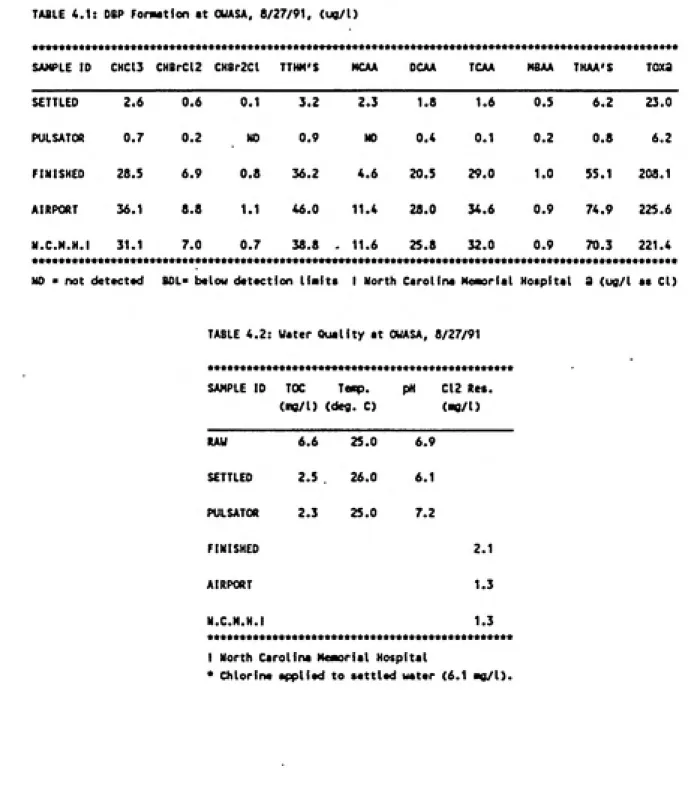
4.1 OWASA
The results of the three sampling visits to the OWASA Water Treatment Plant are contained in Tables 4.1 through 4.6. The results show that the THMs, HAAs and TOX were formed after the chlorine was applied to the settied water and had average concentrations in the distribution system for all three sampling days of 34 ug/1 (TTHMs), 51 ug/1 (THAAs), and 252 ug/1 (TOX). The TOX concentrations ranged fix)m 177 to 310 ug/1, of which 11% was the THMs and 12% was the HAAs, on a chlorine-equivalent basis. Chloroform had the highest concentiation of the THMs at 75% of tiie TTHMs while DCAA and TCAA were tiie major HAA species formed, each accounting for 45% of the THAA concentration.
The WTP operated in the same manner during each sampling visit with an average removal
of TOC of 56% by coagulation and setfling. The only difference in plant operation between
each visit was the amount of chlorine being applied. As expected, the DBF concend-ations
were highest in August and lowest in February, reflecting the decrease in chlorine dosage
(6.1 mg/1 to 3.4 mg/1) as well as the decrease in the water temperature (25 ^C to 15 ^C) (Veenstra and Schnoor, 1980). This is true when the August and February results are compared. However, comparing the August and November results does not show this temperature effect. This may be due to the different TOC concentrations in the settied
TABLE 4.1: OBP Formation at OWASA. 8/27/91, (ug/l)
SAMPLE 10 CHC13 CHBrClZ CHBr2Cl TTHM'S MCAA OCAA TCAA MBAA THAA'S TOxa
SETTLED 2.6 0.6 0.1 3.2 2.3 1.8 1.6 0.5 6.2 23.0
PULSATOK 0.7 0.2 NO 0.9 NO 0.4 0.1 0.2 0.8 6.2
FINISHED 28.5 6.9 0.8 36.2 4.6 20.5 29.0 1.0 55.1 208.1
AIRPORT 36.1 8.8 1.1 46.0 11.4 28.0 34.6 0.9 74.9 225.6
N.C.M.H.I 31.1 7.0 0.7 38.8 - 11.6 25.8 32.0 0.9 70.3 221.4
NO « not detectad BOL- below detection Uaits I North Carolina Meaiorial Hospital a (ug/l as CD
TABLE 4.2: Water Quality at OWASA. 8/27/91
SAMPLE 10 TOC Teaf). pH C12 Res. (Rig/l) (deg. C) (Mg/D
lAU 6.6 25.0 6.9
SETTLED 2.5 26.0 6.1
PULSATOR 2.3 25.0 7.2
FINISHED 2.1
AIRPORT 1.3
N.CM.H.I
********1 >•••*••**« ••**••*••
1.3
I North Carolina Meaiorial Hospital
SAWLE CHC13 CHBrCl2 CNBr2Cl TTHMS MCAA DCAA TCAA H8AA THAA'S Toxa SETTLED 2.9 0.6 NO 3.5 1.2 0.5 0.9 BOL 2.6 31.5
PULSATOR NO NO NO o.» 9.1 0.1 MH. 1.2 35.7
FINISHED 26.3 5.9 1.1 33.3 4.8 19,9 21.3 0.1 46.1 256.9
AtRPOKT 29.6 7.0 1.3 37.9 6.8 24.3 26.0 0.2 57.3 277.0
N.C.M.H.I 28.0 7.2 1.5 36.7 11.7 25.3 26.3 0.2 63.5 310.4
N0« not detected BOL> below detection liait I North Carolina Heiaorial Hoapit 8 (ug/l ae CI)
TABLE 4.4: Water Quality at CUASA, 11/18/91
SAMPLE ID TOC Teinp. pH CL2 Res.
(mg/l) (deg. C) (mg/l)
MU 6.7 18.0 7.5
SETTLED 3.3 18.3 6.6
PULSATOR 3.4 15.0 7.3
FINISHED 1.10
AIRPORT 0.95
N.C.M.H.I
*•••••*•• *•***••*« 0.85 *********** I North Carolina Neaiorial Hospital
TABLE 4.5: MP Fonaation at OUASA. 2/20/92, (ug/l)
SAMPLE CHC13 CHBrCt2 CHBr2Cl TTHM'f MCAA DCAA TCAA HBAA THAA'S Toxa
SETTLED 0.2 0.1 NO 0.3 NO MO
PULSATOR HO NO NO W HD
FINISHED 17.2 6.9 1.0 25.1 80L 15.9
AIRPORT 19.1 7.3 1.0 27.4 2.4 17.7
N.C.N.H.I 18.9 7.4 1.2 27.5 NO 16.1
NO- not datactad lOL- balow dataction liait I North CaroU
BOL NO 8.8
» MO 10.7
13.3 0.1 29.3 177.1
15.6 0.1 35.9 233.9
16.0 0.1 32.3 256.5
fal Hoapital 8 <ag/l aa CI)
TABLE 4.6: Watar Quality at OUASA. 2/20/92
SAMPLE ID TOC Tanp. pH CL2 Ras.
(MO/l) (deg. C) (ag/D
RAW 5.2 15.0 7.2
SETTLED 2.4 15.5 6.3
PULSATOR 2.4 13.5 7.4
EFFLUENT 1.20
AIRPORT t.10
N.C.M.H.I
********4 ••**•••*•
0.90
I North Carolina N«aorial Hospital
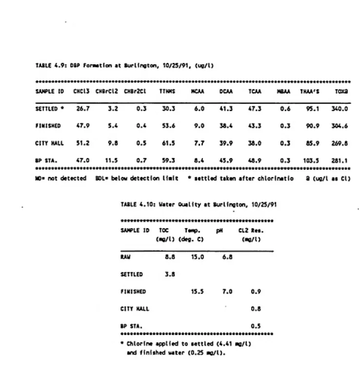
WTP and show the same trends as those observed at OWASA. After the removal of 53%
of the TOC by coagulation and sedimentation, chlorine was applied to the water and the THM, HAA and TOX concentrations increased from this point on, through the treatment plant and out into the distribution system. The TTHM, THAA and TOX concentrations had an average of 42,74 and 226 ug/1 in the distribution system, respectively, where 14% and
18% of the TOX was accounted for by the THMs and HAAs, respectively, on a chlorine-equivalent basis. Chloroform comprised an average of 77% of the THMs, whereas DCAA and TCAA were the principal HAA species at 80% of the THAAs. Chlorine dosage was related to the water temperature, with doses being highest in July when the temperature was high, and lowest in February when the temperature was low. The TOC concentration was
higher in October than in July and February. The relatively high DBP concentrations in the settled water samples in Table 4.9 was the result of the samples having been collected after the chlorine had been applied.
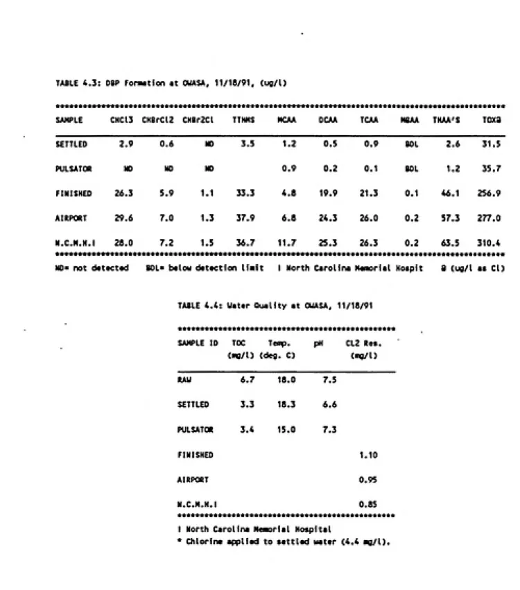
4.3 Durham
The results from the Durham WTPs are presented in Tables 4.13 through 4.18. Removal of 45% of the TOC was accomplished by coagulation and sedimentation before chlorine was applied on top of the filters. This marked the beginning of DBP formation with the TTHM, THAA and TOX concentrations increasing from this point on, with average concentrations in the distribution system of 56,90, and 308 ug/1, respectively. The THMs account for
16% of the TOX on a chlorine-equivalent basis and consisted mostiy of chloroform at 82%. Seventeen percent of the TOX (chlorine-equivalent basis) was comprised of the
HAAs, of which 86% was DCAA and TCAA.
TABLE 4.7: OBP Formation at Burlington, 7/30/91, (ug/l>
SAMPLE 10 CHC13 CHBrCl2 CHBr2Cl TTHM'S NCAA DCAA TCAA MBAA THAA'S TOXS
SETTLED 2.1 0.4 BOL 2.6 6.9 1.0 2.5 BOL 10.4 £;.A
FINISHEO 26,7 6.1 0.8 33.6 21.3 21.0 22.4 0.3 65.1 £-:.7
CITY HALL 37.2 8.5 1.4 47.1 26.3 25.1 29.7 0.4 81.4 241. £
BP STA. 57.0 10.7 1.7 69.3 26.9 28.2 38.4 0.4 93.9 o:- a
NO ͣ not detected BOL> below detection limit* a (ao/t a* CI)
TABLE 4.8: Water Quality at Burlington, 7/30/91
SAMPLE 10 TOG Teap. pH C12 Res. (ͣg/l) (deg. C) (mg/t)
RAW 5.8 25.0 6.5
SETTLED 2.9 7.1
FINISHEO 25.5 7.2 0.9
CITY HALL 0.7
BP STA.
***********>•*•••*•«r*********•*•*••***
0.4
TABLE 4.9: OBP Forawtion at Burlington, 10/25/91, (ug/l)
SAMPLE ID
********
CHC13
*********
CHBrCl2
********************
CHBr2Cl TTHMS
r********i NCAA
k********i
OCAA TCAA NBAA THAA'S Taxa
SETTLED • 26.7 3.2 0.3 30.3 6.0 41.3 47.3 0.6 95.1 340.0
FINISHED 47.9 5.4 0.4 53.6 9.0 38.4 43.3 0.3 90.9 304.6
CITY HALL 51.2 9.8 0.5 61.5 7.7 39.9 38.0 0.3 85.9 269.8
8P STA. 47.0 11.5
*********
0.7 59.3 8.4 45.9 48.9 0.3
•••**•***«••••••••*••*•**••••••••••••••*••••*•*•••«••••
103.5 281.1
••«••***
N0> not detected BOL> below detection lirait * settled taken after chlorinatio a (ug/l a* CI)
TABLE 4.10: Water Quality at Burlington, 10/25/91
SAMPLE ID
>***••*«••••••••••
TOC Tenp. P«
••••••*•*•••
CL2 Re*.
(MB/l) (deg. C) (mg/l)
RAW 8.8 15.0 6.8
SETTLED 3.8
FINISHED 15.5 7.0 0.9
CITY HALL 0.8
BP STA.
••********ik******************••*•***
O.S
************
• Chlorine applied to settled (4.41 ug/l)
TABLE 4.11: OBP Formation at Burlinaton, 2/3/92, (ug/l)
SAMPLE ID CHC13 CHBrClZ CHBr2Cl TTHM'S NCAA DCAA TCAA MSAA THAA'S TOXB
SETTLED 0.4 0.1 NO 0.6 1.3 0.7 0.4 NO 2.5 11.1
FINISHED 14.7 4.6 0.7 20.0 4.8 27.2 19.0 NO S0.9 138.4
CITY HALL 12.3 4.5 0.7 17.5 9.8 23.2 16.0 NO 49.0 149.7
BP STA. 8.3 5.0 1.1 14.4 12.8 19.9 15.7 BOL 48.5 128.2
•a*************************************************************************************************
NO- not detectad BDL> below detaction limit 8 (ug/l as CI)
TABLE 4.12: Water Quality at Burlington, 2/3/92
SAMPLE ID TK T««lp. pH CL2 Re«.
(mg/l) (defl. C) («0/O
RAW 5.7 8.0 6.2
SETTLED 2.7 7.0
FINISHED 12.0 7.0 1.3
CITY HALL 1.2
BP STA. 0.9
BR.SETT 2.6 0.7 BOL 3.3 3.1 0.5 6.0 0.0 10.0 43.8
BR.FIN 35.4 7.5 1.1 43.9 6.2 13.8 42.1 1.4 63.0 267.7
WILL.SETT 2.6 0.6 BOL 3.2 2.3 3.4 3.9 0.1 10.0 86.0
WILL.FIN 46.8 8.5 0.8 56.0 4.9 18.3 58.1 2.3 84.0 291.0
SHELL STA 45.2 9.6 1.1 55.9 10.6 17.1 57.8 2.6 88.0 288.9
CITY HALL 50.0 10.3 1.1 61.4 11.6 21.9 57.1 2.1 93.0 306.8
EPA BLOC 58.2 11.0 1.2 70.5 7.7 19.5 78.7 2.3 108.0 323.9
MO ͣ not detected BOL« bel ow detection limits a (««/t as CD
TABLE 4.14: Water Quality at Ourhaai, 6/18/91
SAMPLE ID TOC Tcaip. pH Cl2 Res.
(ii«/l) (deg. C) (na/l)
BR.RAW 5.0 25.0
BR.SETT 2.9
BR.FIM 2S.0 1.6
WILL.RAW 5.6 23.0
WILL.SETT 3.3
WILL.FIN ».o 2.0
SHELL STA. 1.3
CITY HALL 1.0
EPA BLOC
V*******! »**«*«**«*
0.9
TABLE 4.15: DBP Fonaation at OurhaM, 10/24/91. (ug/l)
SAMPLE ID CHCt3 CHBrClZ CHBrZCl TTHMS NCAA DCAA TCAA MBAA TNAAS TOXa
BA.SETT* 22.2 4.6 0.6 27.3 12.0 19.5 13.1 0.8 45.6 160.3
BR.FIN 59.0 13.9 1.3 74.2 28.0 40.6 29.5 0.5 98.6 232.0
WILL.SETT 7.2 1.0 0.2 8.4 11.0 2.3 1.6 NO 14.8 65.7
WILL.FIN 47.7 12.0 0.9 60.6 15.0 32.6 32.8 0.3 80.4 287.3
SHELL STA 70.1 13.8 2.0 85.8 9.4 39.5 40.9 0.4 90.3 273.1
CITY HALL 54.0 13.3 1.0 68.2 7.2 34.4 38.7 0.5 80.8 250.5
EPA BLOC 69.3 13.6 1.2 84.1 6.8 41.1 44.0 0.4 94.3 324.0
N0« not detected BDL> below detection liMit * BR.SETT after chlorination a (ug/l as Cl>
TABLE 4.16: Water Quality at Ourhaa' 10/24/91
SAMPLE ID TCX: Teaip. pH CL2 Re«.
(ing/l) (deg. C) (Bg/l)
BR.RAW 4.8 21.0 6.9
BR.SETT 5.1 6.4
BR.FIN 18.0 7.1 1.5
WILL.RAW 5.3 22.0 7.0
WILL.SETT 3.4 6.4
WILL.FIN 22.0 7.0 1.8
SHELL STA. 1.0
CITY HALL 1.0
EPA BLDG
»*«*****4»******lk**
0.9
Chlorine applied to settled water:
SAMPLE ID CHC13 CHBrClZ CHir2Ct TTHN'S MCAA DCAA TCAA MBAA THAA'S TOXS
aS.SETT • 8.1
BR.FIN 25.1
WILL.SETT 2.3
WILL.FIN 29.2
SHELL STA 31.2
CITY HALL 32.7
EPA BLDG 40.0
2.0 0.2 10.3 16.3 15.4 13.8
4.4 0.4 29.9 12.8 34.0 33.4
0.3 NO 2.6 8.3 0.8 2.5
4.8 0.3 34.3 17.8 31.3 42.8
6.S 0.4 38.1 15.3 27.8 41.6
6.1 0.3 39.1 15.3 42.4 46.5
4.8 0.4 45.2 11.3 35.7 55.1
NO 45.5 225.0
BOL 80.2 301.9
ND 11.7 92.4
BOL 92.0 287.8
NO 84.8 332.4
BOL 104.2 335.3
NO 102.0 334.4
NO- not detected BOL> below detection liMit * aaiKple taken after chlorination a (ug/l aa CI)
TABLE 4.18: Water Quality at OurhM, 2/4/92
SAMPLE ID TOC Temp. pH CL2 Re«. (MO/l) (deg. C) (Mg/l)
BR.RAW 7.5 12.0
BR.SETT 3.6
BR.FIN 10.0 1.1
WILL.RAW 8.9 13.0
WILL.SETT 4.1
WILL.FIN 9.0 1.5
SHELL STA. 1.0
CITY HALL 0.9
EPA BLDG
»••••*•*<
0.8
* Chlorine afiplied to settled water:
October are not clear. The TOC concentrations were comparable, and although the
temperature was lower on the second day, there was a greater formation of THMs in the
distribution system. It is interesting to note that the THAA concentrations in the distribution
system were similar on all three days.
Overall, the average TOX concentration in the distribution system was 308 ug/1, higher
than either OWASA (252 ug/1) or Burlington (226 ug/1). This can be attributed to the
combination of higher chlorine doses, higher TOC concentrations, and a higher
background concentration of TOX in the settled water prior to chlorine addition. The
Durham WTPs had an average of 3.5 mg/1 of TOC and 70 ug/1 of TOX in their settled
waters while both Chapel Hill and Burlington averaged 2.9 mg/1 and 20 ug/1 of TOC and
TOX, respectively. The reason for the higher settled water TOX in Durham is not clear. It
needs to be noted that these numbers do not include the October and February settled water
results for the Brown plant since the samples were collected after the chlorine had been
applied.
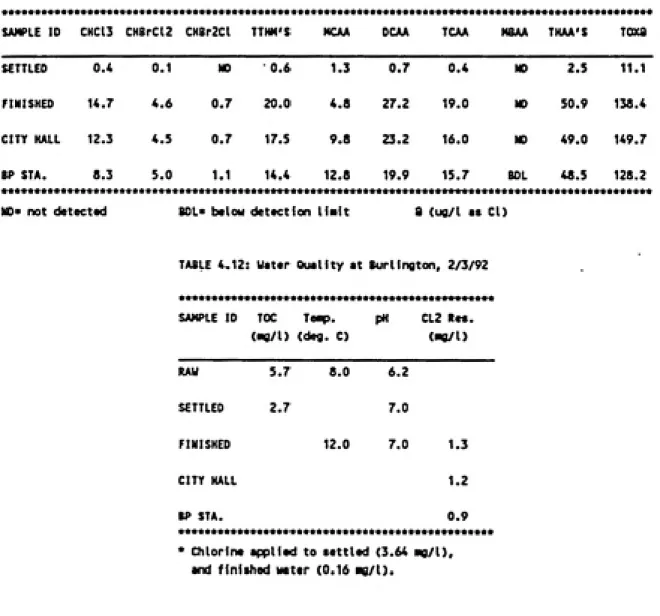
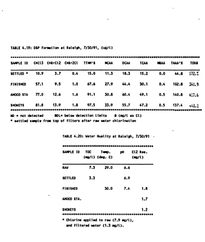
4.4 Raleigh
Tables 4.19 through 4.24, show that the TTHM, THAA, and TOX concentrations
averaged 90, 115, and 385 ug/1, respectively, in the distribution system in July and
October. These concentrations are relatively high, but are consistent with the fact that
chlorine was applied to the raw water on these days, allowing for a longer chlorine contact
time at a higher TOC concentration. Applying chlorine before THM precursor removal by
coagulation results in higher formation of DBFs (Young and Singer, 1979; Jodellah and
Weber, 1985; Chadik and Amy, 1987; Hubel andEdzwald, 1987). In February, the
chlorine was applied on top of the filters, which was later on in the treatment, after 40% of
the TOC had been removed by coagulation and sedimentation. The total chlorine applied to
the water in July and October averaged 9.0 mg/1, much higher than the amount applied in
February of 4.3 mg/1. Subsequently, these changes in operating procedure resulted in less
formation of DBFs in February; the TTHM, THAA, and TOX concentrations in the
distribution system averaged 35,60 and 235 ug/1, respectively. Again, the fraction of TOX
accounted for by the THMs and HAAs was similar to that observed at the other utilities,
TABU 4.19: OtP forMtion at lala<gh, 7/30/91, (ug/l)
SAMPLE 10 CNC13 CHIrClZ CMtrJCl TTHM't NCAA OCAA TCAA MAA TNAA't TOU
KTTLEO • 10.9 3.7 0.4 1S.0 11.3 18.3 15.2 0.0 U.t 172.5
FIHISMCO 57.1 9.5 1.0 67.6 27.9 U.4 30.1 0.4 102.8 341.9
AMOCO STA 77.0 12.6 1.6 91.1 30.8 60.4 49.1 0.5 140.8 417.6
SHOMEYJ 81.8 13.9 1.8 97.5 33.9 55.7 47.2 0.5 137.4 "•a.;
MO - not datactad ML* baloM dataction Malta 8 («g/l •• CD * tattlad ••ͣpi* from top of fittara aftar raw watar ch(or I nation
TABLE 4.20: Watar Ouallty at Ralalgh, 7/30/91
SAMPLE ID TOC Imp. pM C12 la«. (ͣB/t) (ͣe/l) (dag. C)
SETTLED
FINISHED
AMOCO STA.
SHONETS
7.3
3.3
29.0
30.0
6.6
6.9
7.4 1.8
1.7
1.2
* Chtorlna appllad to raw (7.9 hb/I).
TABLE 4.21: DBP FonMtion at Ralalgh. 10/25/91, (uo/l)
•••••••••••••••••*•«*••••••••«*•*••••••••••*•••••*•**••••••*«*•»••••••••••••••••••••••••••••»«••* SAMPLE 10 CHC13 CHBrCl2 CHBr2Cl TTHNS MCAA DCAA TCAA MBAA THAA'S TOXa
RAW* 6.0 1.1 0.1 7.2 1.3 0.3 0.2 NO 1.8 69.6
FINISHED 47.6 13.4 1.2 62.3 10.6 41.9 33.3 0.4 86.2 264.7
A»«XO STA 87.7 19.5 1.8 108.9 5.7 54.5 54.9 0.6 115.8 353.4
SHONEYS 91.0 21.0 1.9 113.9 9.7 47.4 50.9 0.5 108.5 481.5
N0« not detactad BOL* balow detaction liMit a (ug/l a« CI)
* containa filter backwash (chlorinated)
TABLE 4.22: Water Quality at Raleigh, 10/25/91
SAMPLE 10 TOC Temp. pH CL2 Re«.
(MO/l) (deg. C) (MO/l)
RAW 5.3 21.0 6.6 SETTLED 3.6 6.7
FINISHED 20.0 7.5 1.1
AMOCO STA. 0.9 SHONEYS 0.5
TABLE 4.23: DBP Fonnation at Raleigh, 2/3/92, (U0/1)
SAMPLE to CHC13 CHBrCl2 CHBr2Cl TTHM'S NCAA OCAA TCAA MBAA THAA'S Toxa
1 0.9 1.0 NO 11.7 53.3
1 22.5 15.1 SOL 50.4 212.1
1 27.1 20.2 0.2 60.4 255.2
31.9 23.1 0.3 70.7 236.9
a (us/l aa CD SETTLED 0.7 0.4
FINISHED 14.5 9.5
AMOCO STA 20.5 11.3 SHONEYS 29.0 12.7
NO 1.1 9.8
2.5 26.5 12.8
2.8 34.6 12.8 3.2 44.9 15.3
NO- not detected BOL* below detection liait
TABLE 4.24: Water Quality at Raleigh, 2/3/92
SAMPLE ID TOC Teaip. pN CL2 Res.
(lag/l) (deg. C) (Mg/l)
KAtf 6.2 14.0 6.6
SETTLED 3.7 6.8
FINISHED 11.0 7.1 1.2
AMOCO STA. 0.9
SHONEYS
>*••••••< ••«•••••• *••••••**
0.8
* Chlorine applied to aettled (3.0 mg/l),
As in the earlier utilities discussed, decreasing water temperatures were accompanied by
decreasing chlorine doses and resulted in lower formation of DBFs.
4.5 High Point
Tables 4.25 through 4.30 present the results for the three sampling days at the Ward WTP.
The chlorine applied to the settied water (after 29% TOC removal) continued to react with
the NOM present showing increasing DBP concentrations from that point onward. The
average TTHM, THAA and TOX concentrations in the distribution system were 47, 55,
229 ug/1, respectively, where 16% of the TOX was accounted for by the THMs and 14%
by the HAAs on a chlorine-equivalent basis. As observed at the other utilities, chloroform
comprised 79% of the THMs while DCAA and TCAA were equal in concentration,
totalling 95% of tiie HAAs.
In general, a decrease in the water temperature, TOC concentration, and chlorine dose was
reflected by corresponding decreases in the DBP concentrations. The February sample had
a lower water temperature (11 ^C), TOC (2.6 mg/1), and chlorine dose (3.2 mg/1) as
compared to the August sample (28 °C, 3.1 mg/1,6.0 mg/1), respectively, and showed a
corresponding decrease of 50% in the average TTHM, THAA and TOX concentrations in
the distribution system.
4.6 Winston-Salem
The results of the analysis of the water samples collected from the Neilson and Thomas
WTPs in Winston-Salem are presented in Tables 4.31 through 4.36. The Neilson WTP,
which distributes its water to the Etna and BP stations showed a decrease in the THM,
THAA and TOX concentrations as the water temperature and chlorine dose both decreased.
The average THM, HAA and TOX concentrations in the distribution system for the Neilson
WTP decreased from 44 to 16 ug/1, 97 to 25 ug/1, and 195 to 116 ug/1, respectively,
between August and February. A variety of factors can account for this decrease, such as
lower water temperatures and lower chlorine doses, but the most important change between
the two days is believed to be the application of the chlorine on top of the filters instead of
to the raw water. As observed in Raleigh, application after the removal of TOC by
coagulation and settling (35%) results in a significant decrease in DBP formation. The
fraction of the TOX (on a chlorine-equivalent basis) which is comprised of THMs (80%)
TABLE 4.25: DBP FonMtion at High Point, 8/2/91, (ug/l)
SAMPLE ID CHC13 CHBrCl2 CHBr2Cl TTHM'S I4CAA OCAA TCAA MBAA THAA'S TOXa
SETTLED 1.4 0.3 BOL 1.7 HO NO MO K) 18.6
FINISHED 44.3 9.6 1.4 55.2 8.3 27.1 32.9 BOL 68.3 278.8
CITY HALL 54.3 10.7 1.6 66.7 13.6 32.8 36.7 BOL 83.1 292.7
S.E.C.U.I 64.6 12.4 2.0 79.0 4.8 34.7 37.7 BOL 77.2 312.8
NO « not detected BOL ͣ below detection Unit I State Eraployees Credit Union a (ug/l as CI)
TABLE 4.26: Water Quality at High Point, 8/2/91
SAMPLE ID TOC Tenp. pH C12 Res.
(Mg/l) (deg. C) (mg/t)
RAW 4.2 28.0 7.1
SETTLED 3.1 28.0 7.5
FINISHED 28.0 7.6 1.4
CITY HALL 1.0
S.E.C.U. I 0.8
I State Eiiployees Credit Union
TABLE 4.27: DBP Fonaation at High Point, 11/15/91, (ug/l)
SAMPLE CHC13 CHBrClZ CHBrZCl TTHMS NCAA DCAA TCAA NBAA THAA'S TOXS
BOL 2.0 21.7
0.1 46.3 219.5
0.2 54.9 241.7
0.2 53.6 250.0
NO- not detected BOL« below detection liait I State EMployeea Credit Union 8 (ug/l aa CI)
SETTLED NO BOL NO < 0.3 0.9 0.3 0.8
FINISHED 29.3 7.2 1.6 38.1 1.5 19.3 25.3
CITY HALL 36.8 8.1 1.6 46.5 2-2 21.7 30.8
S.E.C.U.I
***********
38.6 8.1 1.7
• •*••••!
48.3 1.6 22.7 29.1
TABLE 4.28: Water Quality at Nigh Point, 11/15/91
SAMPLE ID TOC Taaip. CL2 Re«.
(ͣO/l) (deg. C) (MB/I)
RAU 4.2 14.0 7.1
SETTLED 3.1 14.0 7.8
FINISHED 13.5 7.7 1.0
CITY HALL 0.8
S.E.C.U.I
••••••••••••••••••
0.9
I state Employee* Credit Union