Sequential-Based Approach for Estimating the Stress-Strength Reliability Parameter for Exponential Distribution

DOI:10.29252/jirss.19.1.85

Sequential-Based Approach for Estimating the Stress-Strength

Reliability Parameter for Exponential Distribution

Ashkan Khalifeh1, Eisa Mahmoudi1, and Ali Dolati1

1_{Department of Statistics, Yazd University, Yazd, Iran}

Received: 25/10/2018, Revision received: 15/08/2019, Published online: 26/08/2019

Abstract. In this paper, two-stage and purely sequential estimation procedures are

considered to construct fixed-width confidence intervals for the reliability parameter under the stress-strength model when the stress and strength are independent exponen-tial random variables with different scale parameters. The exact distribution of the stopping rule under the purely sequential procedure is approximated using the law of large numbers and Monte Carlo integration. For the two-stage sequential procedure, explicit formulas for the distribution of the total sample size, the expected value and mean squared error of the maximum likelihood estimator of the reliability parameter under the stress-strength model are provided. Moreover, it is shown that both proposed sequential procedures are finite, and in exceptional cases, the exact distribution of stopping times is degenerate distribution at the initial sample size. The performances of the proposed methodologies are investigated with the help of simulations. Finally using real data, the procedures are clearly illustrated.

Keywords. Law of Large Numbers, Purely Sequential Sampling, Stopping Rule,

Two-stage Sequential Sampling.

MSC:62L15; 60G40; 62F12; 60K10.

Ashkan Khalifeh ([email protected])

Corresponding Author: Eisa Mahmoudi ([email protected]) Ali dolati ([email protected])

1

Introduction

As mentioned in reliability literature, stress-strength models have been described as an assessment of the reliability of a component or system in terms of variables X

indicating stress undertaken by the system andYrepresenting the system’s strength used to endure the stress. Concerning this scenario, the system fails if the stress surpasses the strength. Thus, R = P(X < Y) is the reliability of a system under the stress-strength model. Birnbaum (1956) has introduced the main idea associated with this model. Birnbaum and McCarty (1958) developed this idea using a numerical procedure. Stress-strength models have received notable attention for many years due to their applicability in diverse areas such as medicine, physics, genetics, mechanics as well as in quality control, aerospace engineering, and civil (see, e.g., Domma and Giordano (2013) and Chapter 7 in Kotzet al. (2003)).

The problem of estimatingRhas been widely studied under various distributional assumptions on stress and strength for a variety of data types such as complete data, censored data, and data with explanatory variables, using Monte-Carlo simulation, parametric, nonparametric and Bayesian approaches. For instance, when the independ-ent random variablesXandYfollow the two-parameter exponential distribution, Beg (1980) obtained uniformly minimum variance unbiased estimators (UMVUE) of R. Kundu and Gupta (2006) proposed the maximum likelihood estimator (MLE), two bootstrap confidence intervals and Bayesian estimate of R when the Weibull model holds for stress and strength. When stress and strength are normal or lognormal random variables, Chiodo (2014) discussed a Bayesian inference method for the estimation of the reliability parameter under the stress-strength model. Based on two independent samples from Weinman multivariate exponential distributions with unknown scale parameters, Cramer and Kamps (1997) obtained UMVUE ofP(X<Y) for both, unknown and known common location parameter, under type-II censoring. Awadet al. (1981) and Nadarajah and Kotz (2006) considered a bivariate exponential model for stress and strength.

When stress and strength follow exponential distributions, Tong (1974) derived minimum variance unbiased estimator (MVUE) of R, also several authors discussed evaluation of the mean square error (MSE) of MLE ofR(see, e.g., Kelleyet al. (1976), and Chao (1982)), Moreover Enis and Geisser (1971) applied Bayesian approach to estimate R. Mahmoudi et al. (2018) considered minimum risk sequential point estimation of R and utilized the expected sample size and risk of the sequential procedure. Comprehensive reviews of frequentist inference for stress-strength models are given in Johnson (1988). Kotzet al. (2003) have provided a comprehensive review

of the development of the stress-strength model up to the year 2003. Another review of stress-strength models and interference models are considered by Patowaryet al. (2013).

Govindarajulu (1974) has considered the sequential procedure for the problem of obtaining the confidence interval for the parameterRin three cases, the first of which assumes that (X,Y) follow the bivariate normal distribution and the next two apply the nonparametric approaches. Bandyopadhyayet al. (2003) considered a nonparametric fixed-width confidence interval estimation for the parameterRby adopting a partial sequential sampling scheme. Recently, Mukhopadhyay and Zhuang (2016) have considered a fixed-accuracy interval for the reliability parameter under a bivariate exponential model, namely, the Fisher’s Nile example. Bapat (2018) has constructed a purely sequential estimation methodology to find a fixed-accuracy confidence interval for the unknown parameter R in two separate cases, where (X,Y) have a bivariate exponential distribution due to Marshall and Olkin (1967) and Freund (1961).

As far as we are concerned, there has been no research on sequential analysis for constructing a fixed width confidence interval of the stress-strength reliability parameter, in which the stress and strength distributions are supposed to be exponential. A real example in the composites industry is studied, using the stress-strength model to illustrate the useful application of our proposed method. Referring to Xiaet al. (2009), by using the strengths of two jute fibers possessing two different diameters, say, 10 mm and 20 mm, the reliability parameter under the stress-strength model is analyzed.

In order to construct an asymptotic, fixed-width 2d confidence interval for the stress-strength reliability parameterRby using its MLE, we first need to assess how many samples are needed to construct a 100(1−α_{)% confidence interval. We consider} two sequential procedures and seek to answer the question of whether the procedures attain a prescribed confidence level or not. Regarding this point, the rest of the article is composed of the following sections. In section 2, Asymptotic and exact confidence intervals based on a fixed sample size are introduced. Section 3 introduces a two-stage sequential methodology where the fixed-width 2d(d > 0) confidence interval is considered. In section 4, a purely sequential procedure is defined, and some characteristics of its stopping time are discussed. Moreover, an approximation of the exact distribution of purely sequential procedure, using the law of large numbers is provided. To clarify the theoretical results of the previous sections, we give some simulations in Section 5. In section 6, using real datasets, we illustrate the useful application of our proposed method. Finally section 7, ends with the conclusion.

2

Asymptotic and Exact Confidence Interval Based on a Fixed

Sample Size

In this section, the inferential procedure about the reliability parameter R = P(X < Y), where X and Y are independent, and both have exponential distributions with different scale parameters, is represented based on fixed sample sizes. An exponential distribution denoted by Exp(θ) has the probability density function (pdf) given as follows:

f(x;θ)= 1

θexp(−

x

θ),x>0, θ >0,

whereθis the scale parameter. Let X∼_{Exp (}θ_{1) be independent ofY}∼_Exp(θ_{2), then} the stress-strength reliability parameter can be expressed as follows:

R=P(X<Y)= θ2

θ1+θ2.

Assume that the scale parametersθ1andθ2are both unknown. We want to estimate

stress-strength reliability parameterR=θ2/(θ1+θ2). LetX1, ...,XnandY1, ...,Ynbe two

independent random samples from Exp(θ1) and Exp(θ2), respectively. So, the MLE of Ris

b

Rn=

¯

Yn

¯

Xn+Yn¯ ,

where ¯Xn=n−1Pn

i=1Xiand ¯Yn=n−1Pni=1Yi. Considering the multivariate central limit

theorem (CLT), the asymptotic distribution of ( ¯Xn,Y¯n)T is given by

√

n

_¯

Xn

¯

Yn

!

− θ1

θ2

!!

D

−→_{N2 0},

" θ2

1 0

0 θ2₂

#!

asn−→ ∞,

where N2 denotes bivariate normal distribution and −→D stands for convergence in

distribution. So, the asymptotic distribution of ˆRnis (see Chapter 7 of Ferguson (1996))

√

nbRn−R

D

−→_N

     0,

2θ2₁θ2₂ (θ1+θ2)4

      as n

−→ ∞. _(2.1)

Using (2.1) for a givend >0 andα∈ ₍₀,_{1), a confidence interval forRwith length 2d} based on ˆRn isIn =[ ˆRn−_d,_Rnˆ +_{d]. Limet al. (2004) gave a purely sequential} fixed-width confidence interval estimation procedure for a "smooth" function of the two scale parametersθ1 andθ2 whend −→0. Moreover fordsufficiently small Govindarajulu

(2004) provided a sequential procedure to construct a fixed-width 2dconfidence interval forRwhen (X,Y) has a bivariate normal distribution with an unknown mean vector and an unknown covariance matrix. In this case, if one choosedso large, lower and upper limits of confidence intervalInmight be negative or greater than 1, respectively.

So, assume thatdis sufficiently small (d−→_{0). For the coverage probability (CP) ofIn} with confidence at least 1−α_{, we should have}

P(R∈_In)=_P

bRn

−_R

≤_d

≥₁−α. _(2.2)

Leta=Z1−α/₂>0 be such thatΦ(a)=1−α/2 whereΦ(·) is standard normal cumulative distribution function. For

n∗= 2a 2_θ2

1θ22 d2_(θ

1+θ2)4

,

it follows from (2.1) that oncen∗is sufficiently large, for alln>n∗,

P(R∈_In)=_P

               √

n(bR_n−R) r

2θ2 1θ22 (θ1+θ2)4

≤ √ nd r

2θ2 1θ22 (θ1+θ2)4

               ≥_P                √

n(bR_n−R) r

2θ2 1θ22 (θ1+θ2)4

≤_a               

≈₁−α,

that is, n∗ is the optimal (smallest) fixed sample size, which approximately satisfies (2.2). The exact coverage probability ofInis given in the following theorem.

Theorem 2.1. Let CP(R)=P(R−_d≤_Rˆ_n≤_R+_{d), then}

CP(R)=

      

F_θ1,θ2R1−_d−1;n

−_Fθ

1,θ2

₁

R+d−1;n

R>d

1−_Fθ

1,θ2

₁

R+d −1;n

R≤_d, (2.3)

where F_θ1,θ2(.;n) is the cumulative distribution function (CDF) of random variable Tn =

¯

Xn/Y¯n.

Proof. The proof involves looking at CDF of random variableTn. Let Po(·;µ) denotes

the cumulative distribution function of a Poisson distribution with meanµ. Assume

thatX ∼_{G(h; 1) in whichG(h; 1) stands for a gamma random variable with the shape} parameterhand scale parameter 1. The gamma-Poisson formula (see Kao (1997), p. 51 ) is given by

P(X>x)=Po(h−_1;x), ₀≤_x<∞. _(2.4) LetF_θ1,θ2(t;n)=P(Tn≤t), according to the iterative expectation formula, we have

F_θ1,θ2(t;n)=P

              n P

i=1 Xi n

P

i=1 Yi ≤_t               =E              E               I              n P

i=1 Xi

θ1

≤

tPn

i=1 Yi θ1              n X

i=1 Yi                            ,

where I{} _{is the indicator function. Given that} θ−1

1

Pn

i=1Xi ∼ G(n,1), ¯Xn and ¯Yn are

independent and also using gamma-Poisson formula (2.4), we have

E               I              n P

i=1 Xi

θ1

≤

tPn

i=1 Yi θ1              n X

i=1 Yi= y

              =P               n P

i=1 Xi θ1 ≤ ty θ1              

=1−

n−₁

X

j=0 ytj

expn−yt

θ1

o

θj 1j!

.

Therefore,

F_θ1,θ2(t;n)=1−_E

                      

n−₁

X

j=0 tPn

i=1 Yi !j exp          −

tPn

i=1 Yi θ1          θj

1j!

                      

=1−

n−₁

X

j=0

1

θj 1j!

E                      t n X

i=1 Yi        j exp              −

tPn

i=1 Yi θ1                            .

Now letU=tPn

i=1Yi, obviouslyU∼G(n,1/(tθ2)), so E

Ujexp{−U

θ1

}

=

Z ∞

0

(tθ2)−n Γ(n) u

n−₁

exp{−u

tθ2

}_uj_exp{−u

θ1

}_du

=

Z ∞

0

(tθ2)−n Γ(n) u

n+j−₁

exp{−_u( 1

θ1 +

1

tθ2

)}_du

= Γ(_Γn+j)

(n) (tθ2) −_n

( tθ1θ2

tθ2+θ1

)n+j

= (n+j−1)!

(n−_1)! (

tθ1θ2 tθ2+θ1

)j( θ1

tθ2+θ1

)n. Hence, fort>0

F_θ1,θ2(t;n)=1−

n−₁

X

j=0

(n+j−_1)!

θj

1j!(n−1)!

( tθ1θ2

tθ2+θ1

)j( θ1

tθ2+θ1

)n

=1−

n−₁

X

j=0

n+ j−₁

n−₁

!

tθ2 tθ2+θ1

j

θ

1 tθ2+θ1

n ,

equals 0 fort≤_{0. Remember thatTnis a positive random variable. On the other hand,}

CP(R)=P(R−_d≤_Rˆ_n≤_R+_d)

=P(R−_d≤ 1 1+X¯n

¯ Yn

≤_R+_d)

=

      

P(Tn≤ 1

R−_d −1)−P(Tn≤ _R1+_d−1) R>d 1−_P(Tn≤ 1

R+d−1) R≤d,

which completes the proof.

CDF of the random variable Tn and Theorem 2.1 will come into use in the next

section and along with defining stopping rule (2.5). The required sample size to obtain an exact coverage probability greater than 1−α_is

˜

n(R)=min{_n≥₁|_CP(R)≥₁−α}. _(2.5) Stopping rule (2.5), in which ˆRn=Y¯n/( ¯Xn+Y¯n) is substituted forR, is too complicated

and is asymptotically equivalent to the classical stopping rules based on the asymptotic

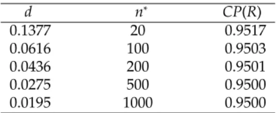
coverage probability. We often have the required coverage whenn ≥_n∗ _{also in small} and medium-size samples. As an example, for α = 0.05, θ1 = 1 and θ2 = 2, by

substitutingn∗fornin (2.3), the results summarized as in Table 1 are acquired.

Table 1: Exact coverage probability for different values ofn∗.

d n∗

CP(R)

0.1377 20 0.9517

0.0616 100 0.9503

0.0436 200 0.9501

0.0275 500 0.9500

0.0195 1000 0.9500

If θ1 andθ2 are known, consequently the asymptotically smallest sample size is

known, and no sequential methods is needed to be applied. The problem of sequential estimation arises when the parameters are unknown. Therefore, two procedures, namely two-stage sequential and purely sequential procedures, are considered for this problem.

3

Two-Stage Sequential Procedure for Fixed-Width Confidence

Interval Estimation of the Stress-Strength Reliability

Parame-ter

LetX1, ...,XmandY1, ...,Ymbe pilot samples of Exp(θ1) and Exp(θ2), respectively. The

statistical and mathematical principles relating to the two-stage procedures have been given by Stein (1945) and are used here to define the stopping rule as follows:

Nm =max

              

2a2X¯2_mY¯2_m d2 _X¯_m+Y¯_m4

       +1,m

      

, (3.1)

whereb_xc_{denotes the largest integer less thanx. IfNm} =_{m, we do not take any more} observations at the second stage. On the other hand, if Nm > m, the initial samples

do not suffice and we then sample the difference (N−_{m) at the second stage. Finally,} sampling stops withX1, ...,XNm,Y1, ...,YNm, and intervalINm =[ ˆRNm−d,RˆNm+d] based on all the 2Nmsamples is proposed forR. Our next goal is to determine the distribution of

Nmusing CDF ofTnand Theorem 2.1, in which the next result deals with this problem.

Throughout this paper,nis an integer number. For eachn<b_a2_/(8d2₎c+_1,anandbnare the real-valued roots of the quadratic equation of the formx2−₍p_2a2_/(d2_l)−_2)x+₁=_0, in whichl=n, (an<bn).

Theorem 3.1. we have the following results:

(i) The probability mass function (PMF) of Nm, in a two-stage procedure is given by

P(Nm=m)=

          

1−_Fθ

1,θ2(bm;m)+Fθ1,θ2(am;m) m<

j _a2 8d2

k

+1

1 m≥j a2

8d2

k

+1,

(ii) If m<j_8da22

k

+1, then the PMF becomes

P(Nm =n)=

              

An m+1≤_n<ja2

8d2

k

+1

F_θ1,θ2(b

a2 8d2

;m)−Fθ

1,θ2(aa2 8d2

;m) n=

j _a2 8d2

k

+1

0 n>j_8da23

k

+1,

where An=Fθ1,θ2(bn−1;m)+Fθ1,θ2(an;m)−

F_θ1,θ2(bn;m)+Fθ1,θ2(an−1;m)

. Proof. (i) Using the CDF ofTnand stopping variable (3.1), we have

P(Nm =m)=P

     

2a2X¯2_mY¯2_m d2 _X¯_m+Y¯_m4

≤_m       =P      T 2 m−       r

2a2 d2_m−2

     Tm+1

≥₀     

. (3.2)

Let∆be equal to the discriminant of the quadratic equation inside (3.2). If∆ is non-positive, thenP(Nm = m) = 1. ∆is non-positive whenm≥ a2/(8d2). It meansNm has

a degenerate distribution atm if and only ifm ≥ b_a2_/(8d2₎c+_1. ∆ _{is positive when}

m<b_a2/_(8d2₎c+_{1, so}

P(Nm=m)=P

     T 2 m−       r

2a2 d2_m−2

     Tm+1

≥₀      

=1−_P(am ≤_Tm ≤_bm)

=1−_Fθ

1,θ2(bm;m)+Fθ1,θ2(am;m).

(ii) Ifm≥ b_a2/_(8d2₎c+_{1, thenNm has a degenerate distribution at initial sample sizem} and consequentlyP(Nm=n)=0 for eachn,m. Form<ba2/(8d2)c+1, the proof is as

follows:

P(Nm =n)=P

     n

−₁≤ 2a

2_X¯2 mY¯2m d2 _Xm¯ _+Ym¯ 4

≤_n       =P      

2a2X¯2_mY¯2_m d2 _Xm¯ _+Ym¯ 4

≤_n       −_P      

2a2X¯2_mY¯2_m d2 _Xm¯ _+Ym¯ 4

≤_n−₁

      =P      T 2 m−       r

2a2 d2_n−2

     Tm+1

≥₀       −_P        

T2_m−

        s

2a2 d2_(n−₁₎−2

       

Tm+1≥₀

        . (3.3)

The first term on the right hand side of (3.3) is equal to 1 when n ≥ _a2_/(8d2_{) and}

the second one is equal to 1 when n ≥ _a2/_(8d2₎ +_{1. So for each n} > b_a2/_(8d2₎c +_1,

P(Nm =n)=0. Letn=b_a2/_(8d2₎c+_{1, then}

P(Nm=n)=P

     T 2 m−       r

2a2 d2_n−2

     Tm+1

≥₀       −_P        

T2_m−

        s

2a2 d2_(n−₁₎−2

       

Tm+1≥₀

       

=1−_[1−_P(an−1≤_Tm ≤_bn−1)]

=F_θ1,θ2(bn−₁;m)−Fθ₁,θ₂(a_n−₁;m)

=F_θ1,θ2(bb_a2_/(8d2₎c;m)−F_θ1,θ2(ab_a2_/(8d2₎c).

Finally, for eachm+1≤_n<b_a2_/(8d2₎c+_1,

P(Nm =n)=P

     T 2 m−       r

2a2 d2_n −2

     Tm+1

≥₀       −_P        

T2_m−

        s

2a2 d2_(n−₁₎−2

       

Tm+1≥₀

       

=P(an−₁ ≤T_m ≤b_n−₁)−P(a_n≤T_m≤b_n)

=F_θ1,θ2(bn−₁;m)+Fθ₁,θ₂(a_n;m)−

F_θ1,θ2(bn;m)+Fθ1,θ2(an−1;m)

.

Theorem 3.1 summarizes by saying that, if starting sample sizem≥ b_a2_/(8d2₎c+_1, then the random variableNmhas a degenerate distribution at the initial sample sizem.

Nm is finite and attains values m, ...,ba2/(8d2)c+1 whenm <ba2/(8d2)c+1. Stopping

ruleNmis the estimate of the unknown optimum sample sizen∗, so we are interested

in computing the expectation of this random variable. The next theorem deals with the expectation of the stopping rule Nm for the case m < ba2/(8d2)c +1, because if m≥ b_a2_/(8d2₎c+_{1, it has been proved in part (i) of Theorem 3.1 thatNmhas a degenerate} distribution atmand henceE[Nm]=m. The following Lemma will help us to compute the expectation of random variableNm.

Lemma 3.1. The cumulative distribution function of Nmis

P(Nm ≤k)=

                      

0 k<m

1−_Fθ

1,θ2(bhki;m)+Fθ1,θ2(ahki;m) m≤k<

j _a2 8d2

k

+1

1 k≥j a2

8d2

k

+1.

(3.4)

Whereh_xi_{denotes the greatest integer less than or equal to x.}

Proof. Ifk < mor k ≥ b_a2/_(8d2₎c+_{1, the proof is evident and the details are avoided.} For the case in whichm≤_k<b_a2_/(8d2₎c+_{1, the proof is as follows:}

P(Nm≤k)=

h_ki

X

i=m

P(Nm =i)

=P(Nm=m)+ h_ki

X

i=m+1

P(Nm =i),

note thatPhki

i=m+1P(Nm =i), is a telescoping series, so we have

h_ki

X

i=m+1

P(Nm=i)=F_θ1,θ2(bm;m)−_Fθ

1,θ2(am;m)+Fθ1,θ2(ahki;m)−Fθ1,θ2(bhki;m). (3.5)

Therefore,

P(Nm≤k)=P(Nm=m)+

h_ki

X

i=m+1

P(Nm =i) =1−_Fθ

1,θ2(bhki;m)+Fθ1,θ2(ahki;m).

Theorem 3.2. For the case m<b_a2/_(8d2₎c+_{1, the expectation of the stopping variable Nm is}

given as

E[Nm]=m+

ba2_/(8d2_)c+1

X

i=m+1

F_θ1,θ2(bi−₁;m)−Fθ₁,θ₂(a_i−₁;m)

. (3.6)

Proof. SinceNm is a discrete random variable with support m,m+1, ...,ba2/8d2c+1,

therefore,

E[Nm]=m+

ba2_/(8d2_)c+1

X

i=m+1

P(Nm≥_i). _(3.7)

Now using Lemma 3.1, we have

P(Nm >k)=

                      

1 k<m

F_θ1,θ2bh_ki;m

−_Fθ

1,θ2

ah_ki;m

m≤_k<ba2

8d2c+1

0 k≥ ba2

8d2c+1.

(3.8)

Hence,

E[Nm]=m+

b_a2_/(8d2₎c+₁

X

i=m+1

P(Nm ≥_i)

=m+P(Nm >m)+P(Nm >m+1)+· · ·+P(Nm >

j

a2/(8d2)k)

=m+

ba2/(8d2)c₊1

X

i=m+1

F_θ1,θ2(bi−₁;m)−Fθ₁,θ₂(a_i−₁;m)

.

Theorem 3.3. The first and second moments ofRˆNm are, given respectively by

EhbR_Nm i

=

ba2_/(8d2_)c+1

X

n=m

k(n, ρ)

B(n,n)P(Nm=n), (3.9)

where

k n, ρ= Z 1

0

tn(1−_t)n−1

ρ+ 1−ρ

tdt,

ρ=θ1/θ2and B(·,·)is Euler’s integral of the first kind (also known as beta function), and

EhbR2_N m

i

=

ba2_/8d2_c+1

X

n=m

"

n(1+ρ) 1−ρ +1

!

k(n, ρ)

B(n,n) −

n

1−ρ

#

P(Nm =n). (3.10)

Proof. According to Sathe and Shah (1981), we have

EhbR_n i

= k(n, ρ) B(n,n), and

EhbR2_n i

= n(1+ρ)

1−ρ +1

!

k(n, ρ)

B(n,n) −

n

1−ρ. So,E[ ˆRNm] andE[ ˆR2_Nm] are given, respectively by

EhbR_Nm i

=E

E

b

RNm Nm

=E

"

k(Nm, ρ) B(Nm,Nm)

#

=

ba2_/8d2_c+1

X

n=m

k(n, ρ)

B(n,n)P(Nm=n), and

EhbR2_N m

i

=E

E

bR2_N

m Nm

=E

"

Nm(1+ρ) 1−ρ +1

!

k(Nm, ρ)

B(Nm,Nm)

− Nm

1−ρ

#

=

ba2_/(8d2_)c+1

X

n=m

"

n(1+ρ) 1−ρ +1

!

k(n, ρ)

B(n,n) −

n

1−ρ

#

P(Nm=n).

Using Theorem 3.3 the MSE of ˆRNmaccording toRis given by

MSEhbRN_m i

=EhbR2_N m

i

−_2REhbRN_m i

+R2. (3.11)

Theorem 3.4. The coverage probability( ˆRNm−d,RˆNm+d)is as follows:

CP(R)=

ba2/(8d2)c₊1

X

n=m

F_θ1,θ2( 1

R−_d−1;n)−Fθ1,θ2(

1

R+d −1;n)P(Nm=n)

I{_R>_d}

+

ba2_/(8d2_)c+1

X

n=m

1−_Fθ

1,θ2(

1

R+d−1;n)P(Nm =n)

I{_R≤_d}. _(3.12)

Proof. Using Theorem (2.1) and iterative expectation formula, we have

CP(R)=PR−_d≤_RNˆ

m ≤R+d

=EnEhI{_R−_d≤_RNˆ

m ≤R+d}

Nm

io

=E[

F_θ1,θ2( 1

R−_d −1;Nm)−Fθ1,θ2(

1

R+d −1;Nm)

I{_R>_d}

+1−_Fθ

1,θ2(

1

R+d−1;Nm)

I{_R≤_d}_]

=

ba2_/8d2_c+1

X

n=m

F_θ1,θ2( 1

R−_d−1;n)−Fθ1,θ2(

1

R+d −1;n)P(Nm=n)

I{_R>_d}

+

ba2/8d2c₊1

X

n=m

1−_Fθ

1,θ2(

1

R+d −1;n)P(Nm =n)

I{_R≤_d}.

4

Purely Sequential-Based for Fixed-Width Confidence Interval

Estimation of the Stress-Strength Reliability Parameter

estimates the required sample size, Nm using a small number of observations as, m. However, the procedure tends to oversample and the amount of oversampling increases with the increase in (Nm −_{m). To reduce oversampling by the two-stage} procedure, we have to proceed the estimation ofRsuccessively in a sequential manner. We begin with a few observations (say, m > 2) and then we continue to take one additional observation at-a-time, but terminate sampling when we have gathered enough observations. As soon as a sample size exceeds the corresponding estimate of

n∗, the sampling is terminated right there, and an interval estimator ofRis constructed. In this section, a sequential procedure for estimating the stress-strength reliability parameter for exponential distributions is proposed, and using the law of large numbers, the characteristics of its stopping time are depicted. First, note that

Nd=min

      

n≥_m

n≥ 2a

2_X¯2 nY¯2n d2 _X¯_n+Y¯_n4

       , (4.1)

in whichm ≥_{2 is the starting (or pilot) sample size. Nd can be expressed in terms of}

Tn=X¯n/Y¯nas follows:

Nd =min

      

n≥_m

¯

Xn+Y¯n4

¯

X2_nY¯2_n

≥ 2a

2 nd2        =min       

n≥_m

T2_n−₍

r

2a2

nd2 −2)Tn+1≥0

       . (4.2)

Note that there is no real solution to the quadratic equation inside (4.2) forn>a2/8d2.

Theorem 4.1. Let al and bl be the real-valued roots of the quadratic equation inside (4.2) for

n=l, such that a_l<b_l, then (i)

P(Nd=m)=

          

1−_P(am ≤_Tm ≤_{bm) m}<ja2

8d2

k

+1

1 m≥ja2

8d2

k

+1,

(ii)

P(Nd≤k)=

              

0 k<m

1−_P h_ki

T

i=m

{_ai ≤_Ti ≤_bi}

!

m≤_k<ja2

8d2

k

+1

1 k≥ja2

8d2

k

+1.

Proof. (i) The discriminant of the quadratic equation inside (4.2) is non-positive for,

n ≥_a2/_(8d2_{). It means that for eachn}≥ _a2/_(8d2_{) ,T}2

n−(

p

2a2_/(nd2₎−_2)Tn+₁ ≥_{0. So} for each n ≥ _m ≥ b_a2_/(8d2₎c+_{1, the quadratic equation inside (4.2) is non-negative.} Therefore, the minimumn ≥ _{msuch thatT}2

n−(

p

2a2_/(nd2₎−_2)Tn+₁ ≥ _{0 ismitself.} Thus ifm≥ b_a2/_(8d2₎c+_{1, thenP(Nd}=_m)=_{1 and ifm}<b_a2/_(8d2₎c+_1,

P(Nd =m)=P

     T 2 m−(

r

2a2

md2 −2)Tm+1≥0

     

=1−_P(am ≤_Tm≤_bm). (ii) It is apparent thatP(Nd≤k)=0 ifk<m. Form≤k<

j

a2/(8d2)k+1,

P(Nd >k)=P(Nd,m, ...,Nd,k)

=P       

h_ki

\

i=m

      

T_i2−₍

r

2a2

id2 −2)Tn+1<0

              =P       

h_ki

\

i=m

{_ai≤_Ti≤_bi}

       .

Finally, if k = b_a2/_(8d2₎c+_{1, in the view of the fact that for eachn} ≥ _a2/_(8d2_{) , T}2

n−

(p2a2/_(nd2₎−_2)Tn+_{1>0 (see part (i)), then we have}

P(Nd≤

$

a2

8d2

%

+1)=1−_{P Nd} >

$

a2

8d2

%

+1

!

=1−_{P(Nd ,m}, ...,_Nd,

$

a2

8d2

%

+1)

=1−_P

          

ba2

8d2c+1 \

i=m

      

T_i2−₍

r

2a2

id2 −2)Tn+1<0

                 

=1. So, ifk=b_a2_/(8d2₎c+_{1 thenT}2

k−(

p

2a2_/(kd2₎−_2)Tk+_{1>0, the intersection is an empty}

set, which is the desired result.

Part (i) of Theorem 4.1 shows that if the starting sample sizem≥ b_a2/_(8d2₎c+_{1, then}

Nd has a degenerate distribution atm. Part (ii) of Theorem 4.1 indicates that Nd can

attain valuesm,m+1, ...,b_a2/_(8d2₎c+_{1, proving that not onlyP(Nd} < ∞₎ = _{1 but also}

P(Nd≤ ba2/(8d2)c+1)=1.

We can approximateP(Nd>k), by using the law of large numbers. Using part (ii)

of Theorem 4.1, for eachm≤_k<b_a2_/(8d2₎c+_{1, we have}

P(Nd>k)=P

      

h_ki

\

i=m

{_ai ≤_Ti ≤_bi}

       =E        I       

h_ki

\

i=m

{_ai ≤_Ti≤_bi

              .

In order to apply the strong law of large numbers, we only need to show that

E[|_I{Thki

i=m{ai ≤Ti≤bi}|]<∞, which in this case is trivial because|I{

Thki

i=m{ai ≤Ti ≤bi}}| ≤

1. It may be observed that, generating random numbers from the joint distribution of (Tm, ...,Th_ki) is very straightforward by using the definition of (Tm, ...,Th_ki). More precisely, first generateX1, ...,Xh_kiandY₁, ...,Yh_kifrom Exp(θ₁) and Exp(θ₂) distributions, respectively. Then set

Tj= j

P

i=1 Xi j

P

i=1 Yi

, j=m, ...,h_ki.

Now, lettm=(tm1, ...,tmn) benindependent observations fromTm. Using Monte Carlo

integration, for sufficiently largen(n−→ ∞_{), we have}

b

P(Nd >k)=

1

n n

X

j=1 I        k \

i=m

n

ai ≤ti j≤bi

o        −→_E        I        k \

i=m

{_ai ≤_Ti ≤_bi

             

=P(Nd>k).

Therefore, using part (ii) of Theorem 3.4 and Monte Carlo method, we can approximate the CDF ofNdas follows:

bP(N_d≤k)=           

0 k<m

1−_bP(Nd>_{k) m}≤_k<j a2

8d2

k

+1

1 k≥j a2

8d2

k

+1,

So,bP(N_d=n)=bP(N_d≤n)−bP(N_d ≤n−1). Having approximated the exact distribution

ofNd, we can estimate the average stopping time, the average estimate ofR, MSE ofbR_Nd

according toRand the coverage probability ofR. LetbP(N_d =n) be the approximation

ofP(Nd=n), so we approximate the average stopping time,E[Nd] byE[Nd]∗as follows:

E[Nd]

∗

=

ba2_/8d2_c+1

X

i=m

ibP(N_d=i). (4.3)

To approximate E[ ˆRNd], E[ ˆR

2

Nd], MSE of ˆRNd according to R and CP, we use (3.9)-(3.12), respectively, in whichNd is substituted forNm andbP(N_d =n) is substituted for

P(Nm =n). So we have

EhbRN_d i∗

=

ba2/(8d2)c₊1

X

n=m

k(n, ρ)

B(n,n)bP(Nd=n), (4.4)

EhbR2_N d

i∗

=

ba2_/8d2_c+1

X

n=m

"

n(1+ρ) 1−ρ +1

!

k(n, ρ)

B(n,n) −

n

1−ρ

# b

P(Nd=n), (4.5)

and the MSE of ˆRNd according toRis

MSEbR_Nd ∗

=EhbR2_N d

i∗

−_2REh_bRN d

i∗

+R2. (4.6)

Finally, the CP is as follows:

CP(R)∗=

ba2_/(8d2_)c+1

X

n=m

F_θ1,θ2( 1

R−_d −1;n)−Fθ1,θ2(

1

R+d−1;n)bP(Nd=n)

I{_R>_d}

+

ba2_/(8d2_)c+1

X

n=m

1−_Fθ

1,θ2(

1

R+d −1;n)bP(Nd=n)

I{_R≤_d}. _(4.7)

5

Computation and Simulation Results

We have done detailed computations to justify the results of the previous sections, but for the sake of brevity, we only present a summary here. Purely and two-stage procedures are considered whenθ1 =1 andθ2 =2, 3, 5 and 7, the confidence level is

1−α=₀._{95, the initial sample sizem}=_{5, 10, 20 anddis chosen such thatn}∗₌

20, 100, 200,

500 and 1000. For each set of values, we ranh=10,000 replications by letting MATLAB ("MATLAB 2018a, The MathWorks, Natick, 2018") draw samples from the preassigned exponential populations. Suppose that in theith replication there areni observations. Based on these data, we estimate R by ¯Yni/( ¯Xni +Y¯ni). That is, for the two stage sequential procedures; we observedNm =ni and set ˆRNm =Y¯ni/( ¯Xni+Y¯ni). Similarly, for the purely sequential procedures, we observedNd=niand set ˆRNd =Yn¯ i/( ¯Xni+Yn¯ i). The distribution ofNdfor the purely sequential procedure is approximated using 10,000

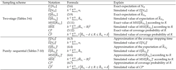
replications. Table 2 represents the notations used to summarize our results.

Table 2: Index of notation that is used in Table 3-10.

Sampling scheme Notation Formula Explain

Two-stage (Tables 3-6)

E[Nm] (3.6) Exact expectation ofNm

b

E[Nm] h−1Ph_i=1ni Simulated value ofE[Nm]

E[bR_Nm] (3.9) Exact expectation ofbR_Nm b

E[bR_Nm] h −₁Ph

i=1Rˆni Simulated value of expectation ofbR_Nm

MSE[bR_Nm] (3.11) Exact value ofMSE[bR_Nm] according toR

[

MSE h−₁Ph

i=1( ˆRni−R)2 Simulated value ofMSE[bR_Nm] according toR

CP (3.12) Exact value of coverage probability ofR

c

CP h−₁Ph i=1I

n

ˆ

Rni−d≤R≤Rˆni+d o

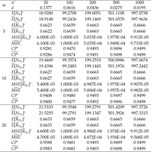
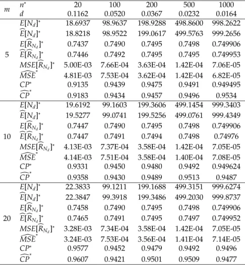
Simulated value of coverage probability ofR

Purely- sequential (Tables 7-10) E[Nd]

∗

(4.3) Approximation of the average stopping time

b

E[Nd]∗ h−1P_i=h1ni Simulated value ofE[Nd]∗

E[bR_N d]

∗

(4.4) Approximation of the expectation ofbR_N d b

E[bR_N d]

∗

h−₁Ph

i=1Rˆni Simulated value ofE[bR_N d]

∗ MSE[bR_Nd]

∗

(4.6) Approximation ofMSE[ ˆRNd] according toR

[

MSE ∗

h−1Ph

i=1( ˆRni−R)

2 _{Simulated value ofMSE[ ˆR}

Nd] ∗

according toR CP∗

(4.7) Approximation of coverage probability ofR

c

CP ∗

h−₁Ph i=1I

n

ˆ

Rni−d≤R≤Rˆni+d o

Simulated value ofCP∗

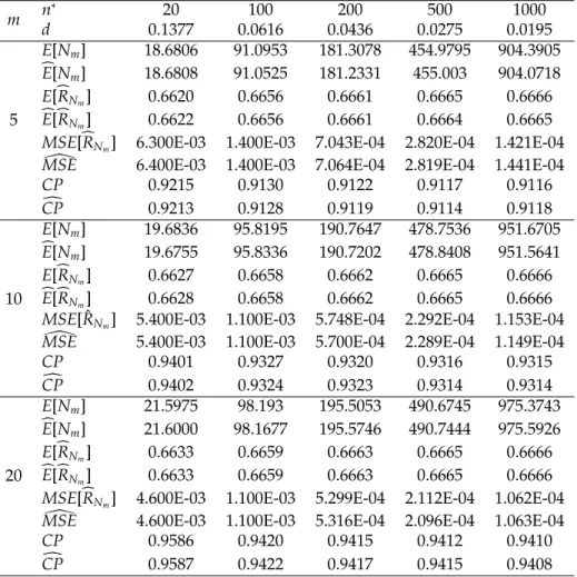
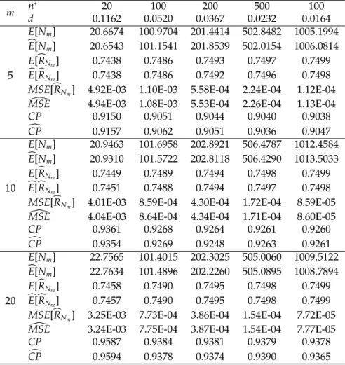
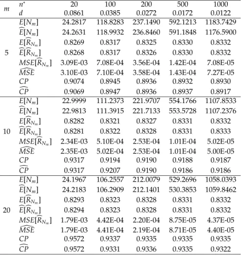
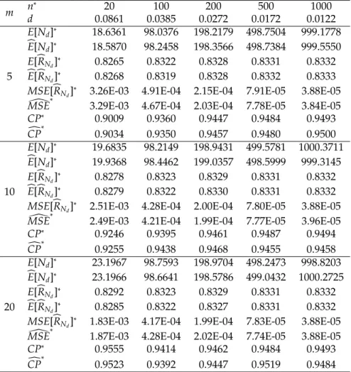
As Tables 3-10 show, the accuracy, precision, and coverage probability increase with

m. The coverage probability is below the target for some cases, so we need to find the initial sample sizem in such a way that the coverage probability gets at least 1−α_. We considered it only for the two-stage sequential procedure because we have found an exact distribution only for this case. Table 11, indicates the characteristic of the two-stage procedure and the smallestmsuch that the coverage probability be at least 1−α_{. In Table 11, oversampling by the two-stage procedure is obvious. Some of the} main results of the simulations are listed as follows:

1. The results derived from both of the proposed sequential procedures are almost

the same.

2. For both proposed sequential procedures, the results of simulations and exact computations (approximations) are extremely coincide with each other, confirming the theorem’s accuracy mentioned in the previous sections.

3. Given a fixed value ofm, asddecreases,E[Nm] andE[ ˆRNm] increase withE[ ˆRNm] gets closer toR. Similarly,E[Nd]∗andE[ ˆRNd]

∗

increase, withE[ ˆRNd] ∗

nearing toR.

4. Given either a fixed or decreasing value ofd, as the initial sample size,mincreases,

CP(CP∗

) increases, and nears its nominal value to 1−α_.

5. Comparing the results in Tables 3-6 (two-stage procedure) and Tables 7-10 ( purely sequential procedure) we realize that, in the cases examined, the expected sample size in the two-stage procedure is generally larger thann∗, whereas in the sequential procedure it is generally smaller thann∗

. The bias of the estimators ofRis negative in both procedures and is almost the same magnitude. Similar results is found about the MSE of the estimators. The coverage probabilities in both procedures are generally below the prescribed 1−α_{value. These values} approach the prescribed values, asmgetting larger. The coverage probability in the sequential procedure is more than the coverage probability in the two-stage procedure. In all cases, the purely sequential procedure is more efficient.

Although we approximate the exact distribution ofN_d, one may notice that purely sequential strategy outperforms the two-stage sequential estimation strategy. Indeed, both procedures are fully expected to perform very well, but the two-stage sequential procedure is logistically more straightforward to be implemented than a purely sequential estimation one. Based on the simulation results, we can conclude that the proposed sequential procedures are working quite well, and they can be used quite effectively for data analysis purposes.

Table 3: Characteristics and simulated values of two-stage procedure withα = 0.05,

θ1=1,θ2=2,m=5, 10, 20 andR=0.6666.

m n

∗

20 100 200 500 1000

d 0.1377 0.0616 0.0436 0.0275 0.0195

5

E[Nm] 18.6806 91.0953 181.3078 454.9795 904.3905

b

E[Nm] 18.6808 91.0525 181.2331 455.003 904.0718 E[bR_Nm] 0.6620 0.6656 0.6661 0.6665 0.6666 b

E[bRNm] 0.6622 0.6656 0.6661 0.6664 0.6665

MSE[bRNm] 6.300E-03 1.400E-03 7.043E-04 2.820E-04 1.421E-04

[

MSE 6.400E-03 1.400E-03 7.064E-04 2.819E-04 1.441E-04

CP 0.9215 0.9130 0.9122 0.9117 0.9116

c

CP 0.9213 0.9128 0.9119 0.9114 0.9118

10

E[Nm] 19.6836 95.8195 190.7647 478.7536 951.6705

b

E[Nm] 19.6755 95.8336 190.7202 478.8408 951.5641 E[bRNm] 0.6627 0.6658 0.6662 0.6665 0.6666 b

E[bRNm] 0.6628 0.6658 0.6662 0.6665 0.6666

MSE[ ˆRNm] 5.400E-03 1.100E-03 5.748E-04 2.292E-04 1.153E-04

[

MSE 5.400E-03 1.100E-03 5.700E-04 2.289E-04 1.149E-04

CP 0.9401 0.9327 0.9320 0.9316 0.9315

c

CP 0.9402 0.9324 0.9323 0.9314 0.9314

20

E[Nm] 21.5975 98.193 195.5053 490.6745 975.3743

b

E[Nm] 21.6000 98.1677 195.5746 490.7444 975.5926 E[bR_Nm] 0.6633 0.6659 0.6663 0.6665 0.6666 b

E[bRNm] 0.6633 0.6659 0.6663 0.6665 0.6666

MSE[bRNm] 4.600E-03 1.100E-03 5.299E-04 2.112E-04 1.062E-04

[

MSE 4.600E-03 1.100E-03 5.316E-04 2.096E-04 1.063E-04

CP 0.9586 0.9420 0.9415 0.9412 0.9410

c

CP 0.9587 0.9422 0.9417 0.9415 0.9408

Table 4: Characteristics and simulated values of two-stage procedure withα = 0.05,

θ1=1,θ2 =3,m=5, 10, 20 andR=0.7500.

m n

∗

20 100 200 500 100

d 0.1162 0.0520 0.0367 0.0232 0.0164

5

E[Nm] 20.6674 100.9704 201.4414 502.8482 1005.1994

b

E[Nm] 20.6543 101.1541 201.8539 502.0154 1006.0814 E[bR_Nm] 0.7438 0.7486 0.7493 0.7497 0.7499 b

E[bRNm] 0.7438 0.7486 0.7492 0.7496 0.7498

MSE[bRNm] 4.92E-03 1.10E-03 5.58E-04 2.24E-04 1.12E-04

[

MSE 4.94E-03 1.08E-03 5.53E-04 2.26E-04 1.13E-04

CP 0.9150 0.9051 0.9044 0.9040 0.9038

c

CP 0.9157 0.9062 0.9051 0.9036 0.9047

10

E[Nm] 20.9463 101.6958 202.8921 506.4787 1012.4584

b

E[Nm] 20.9310 101.5722 202.8118 506.4290 1013.5033 E[bRNm] 0.7449 0.7489 0.7494 0.7498 0.7499 b

E[bRNm] 0.7451 0.7488 0.7494 0.7497 0.7498

MSE[bRNm] 4.01E-03 8.59E-04 4.30E-04 1.72E-04 8.59E-05

[

MSE 4.04E-03 8.64E-04 4.34E-04 1.71E-04 8.60E-05

CP 0.9361 0.9268 0.9264 0.9261 0.9260

c

CP 0.9354 0.9269 0.9248 0.9263 0.9261

20

E[Nm] 22.7565 101.4015 202.3025 505.0060 1009.5122

b

E[Nm] 22.7634 101.4896 202.2260 505.0895 1008.7894 E[bRNm] 0.7458 0.7490 0.7495 0.7498 0.7499 b

E[bRNm] 0.7457 0.7490 0.7495 0.7498 0.7499

MSE[bRNm] 3.25E-03 7.73E-04 3.86E-04 1.54E-04 7.72E-05

[

MSE 3.24E-03 7.75E-04 3.87E-04 1.54E-04 7.77E-05

CP 0.9587 0.9384 0.9381 0.9379 0.9378

c

CP 0.9594 0.9378 0.9374 0.9390 0.9365

Table 5: Characteristics and simulated values of two-stage procedure withα = 0.05,

θ1=1,θ2=5,m=5, 10, 20 andR=0.8333.

m n

∗

20 100 200 500 1000

d 0.0861 0.0385 0.0272 0.0172 0.0122

5

E[Nm] 24.2817 118.8283 237.1490 592.1213 1183.7429

b

E[Nm] 24.2631 118.9932 236.8460 591.1848 1176.5900 E[bR_Nm] 0.8269 0.8317 0.8325 0.8330 0.8332 b

E[bRNm] 0.8268 0.8317 0.8326 0.8330 0.8332 MSE[bRNm] 3.09E-03 7.08E-04 3.56E-04 1.42E-04 7.08E-05

[

MSE 3.10E-03 7.10E-04 3.58E-04 1.43E-04 7.27E-05

CP 0.9074 0.8945 0.8936 0.8932 0.8930

c

CP 0.9069 0.8947 0.8936 0.8937 0.8917

10

E[Nm] 22.9999 111.2373 221.9707 554.1766 1107.8533

b

E[Nm] 22.9813 111.3915 221.7133 553.5728 1107.2376 E[bRNm] 0.8282 0.8321 0.8327 0.8331 0.8332

b

E[bRNm] 0.8281 0.8322 0.8328 0.8331 0.8333 MSE[bRNm] 2.34E-03 5.10E-04 2.53E-04 1.01E-04 5.02E-05

[

MSE 2.35E-03 5.02E-04 2.53E-04 1.01E-04 5.00E-05

CP 0.9317 0.9194 0.9190 0.9188 0.9187

c

CP 0.9317 0.9207 0.9190 0.9186 0.9186

20

E[Nm] 24.1967 106.2557 212.0079 529.2696 1058.0393

b

E[Nm] 24.2183 106.2909 212.1401 530.3853 1059.8462 E[bRNm] 0.8293 0.8323 0.8328 0.8331 0.8332

b

E[bRNm] 0.8294 0.8323 0.8328 0.8331 0.8332 MSE[bRNm] 1.79E-03 4.42E-04 2.20E-04 8.75E-05 4.37E-05

[

MSE 1.79E-03 4.41E-04 2.19E-04 8.71E-05 4.40E-05

CP 0.9572 0.9337 0.9335 0.9335 0.9335

c

CP 0.9572 0.9331 0.9336 0.9335 0.9322

Table 6: Characteristics and simulated values of two-stage procedure withα = 0.05,

θ1=1,θ2 =7,m=5, 10, 20 andR=0.875.

m n

∗

20 100 200 500 1000

d 0.0678 0.0303 0.0214 0.0136 0.0096

5

E[Nm] 27.1543 133.0503 265.5876 663.2155 1325.9306

b

E[Nm] 27.1849 132.9368 266.0099 663.1108 1329.4560 E[bR_Nm] 0.8690 0.8735 0.874217 0.8747 0.8748 b

E[bRNm] 0.8689 0.8734 0.874237 0.8747 0.8748

MSE[bRNm] 2.10E-03 4.84E-04 2.42E-04 9.60E-05 4.76E-05

[

MSE 2.09E-03 4.84E-04 2.40E-04 9.56E-05 4.84E-05

CP 0.9038 0.8887 0.887705 0.8872 0.8871

c

CP 0.9042 0.8882 0.88737 0.8869 0.8865

10

E[Nm] 24.4308 117.9825 235.4582 587.8949 1175.2899

b

E[Nm] 24.3310 118.0597 235.364 588.6521 1177.0300 E[bRNm] 0.8704 0.8739 0.874449 0.8748 0.8749 b

E[bRNm] 0.8705 0.8738 0.874447 0.8748 0.8749

MSE[bRNm] 1.51E-03 3.32E-04 1.64E-04 6.50E-05 3.24E-05

[

MSE 1.49E-03 3.34E-04 1.65E-04 6.57E-05 3.27E-05

CP 0.9296 0.9153 0.914875 0.9147 0.9146

c

CP 0.9300 0.9146 0.91502 0.9131 0.9148

20

E[Nm] 25.0496 109.4479 218.3886 545.2214 1089.9429

b

E[Nm] 25.0325 109.3863 218.7623 546.4983 1093.5911 E[bRNm] 0.8714 0.8741 0.874528 0.8748 0.8749 b

E[bRNm] 0.8715 0.8740 0.874464 0.8748 0.8749

MSE[bRNm] 1.12E-03 2.81E-04 1.39E-04 5.54E-05 2.76E-05

[

MSE 1.12E-03 2.83E-04 1.39E-04 5.49E-05 2.73E-05

CP 0.9561 0.9310 0.930961 0.9310 0.9310

c

CP 0.9574 0.9308 0.93061 0.9324 0.9319

Table 7: Characteristics and simulated values of purely sequential procedure with

α=0.05,θ1=1,θ2 =2,m=5, 10, 20 andR=0.6666.

m n

∗

20 100 200 500 1000

d 0.1377 0.0616 0.0436 0.0275 0.0195

5

E[Nd]∗ 18.9280 99.2708 199.0051 501.1108 997.0738

b

E[Nd]∗ 18.9148 99.2436 199.1469 501.6570 997.9636 E[bR_Nd]∗ 0.6623 0.6659 0.6663 0.6665 0.6666 b

E[bRNd]∗ 0.6622 0.6659 0.6663 0.6665 0.6666 MSE[bRNd]

∗

6.000E-03 1.000E-03 5.033E-04 1.975E-04 9.912E-05 [

MSE∗ 6.100E-03 1.000E-03 5.035E-04 1.949E-04 9.733E-05

CP∗ 0.9281 0.9470 0.9493 0.9496 0.9499

d

CP∗ _{0.9286 0.9474 0.9491 0.9498 0.9498}

10

E[NNd] ∗

19.4449 99.3574 199.2510 500.8986 997.0674 b

E[NNd]∗ 19.4396 99.2483 199.1443 501.1976 997.2442 E[bRNd]∗ 0.6627 0.6659 0.6663 0.6665 0.6666

b

E[bRNd]∗ 0.6627 0.6659 0.6663 0.6665 0.6666 MSE[bRNd]

∗

5.400E-03 1.000E-03 4.987E-04 1.975E-04 9.907E-05 [

MSE∗ 5.400E-03 1.000E-03 5.006E-04 1.957E-04 9.982E-05

CP∗

0.9408 0.9480 0.9493 0.9497 0.9499

d

CP∗

0.9400 0.9477 0.9492 0.9496 0.9498

20

E[NNd]∗ 21.5103 99.3548 199.2791 501.4209 997.3726

b

E[NNd]∗ 21.5255 99.2791 199.1347 501.3926 997.3315 E[bRNd]∗ 0.6633 0.6659 0.6663 0.6665 0.6666

b

E[bRNd] ∗

0.6633 0.6659 0.6663 0.6665 0.6666

MSE[bR_Nd]∗ 4.600E-03 1.000E-03 4.986E-04 1.974E-04 9.912E-05 [

MSE∗ 4.700E-03 1.000E-03 4.872E-04 1.934E-04 9.568E-05

CP∗

0.9588 0.9481 0.9493 0.9499 0.9499

d

CP∗ _{0.9583 0.9481 0.9493 0.9498 0.9499}

Table 8: Characteristics and simulated values of purely sequential procedure with

α=0.05,θ1=1,θ2=3,m=5, 10, 20 andR=0.7500.

m n

∗

20 100 200 500 1000

d 0.1162 0.0520 0.0367 0.0232 0.0164

5

E[Nd]∗ 18.6937 98.9637 198.9288 498.8600 998.2622

b

E[Nd]∗ 18.8218 98.9522 199.0617 499.5763 999.2656 E[bR_Nd]∗ 0.7437 0.7490 0.7495 0.7498 0.749906 b

E[bRNd]∗ 0.7446 0.7492 0.7495 0.7495 0.749953 MSE[bRNd]

∗

5.00E-03 7.66E-04 3.63E-04 1.42E-04 7.06E-05 [

MSE∗ 4.81E-03 7.53E-04 3.62E-04 1.42E-04 6.82E-05

CP∗ 0.9135 0.9439 0.9475 0.9491 0.949495

c

CP∗ 0.9183 0.9434 0.9457 0.9496 0.9534

10

E[Nd]∗ 19.6192 99.1603 199.3606 499.1454 999.3403

b

E[Nd]∗ 19.5277 99.0741 199.5256 499.0761 999.4349 E[bRNd]∗ 0.7447 0.7490 0.7495 0.7498 0.749906

b

E[bR_Nd]∗ 0.7447 0.7491 0.7494 0.7498 0.74976

MSE[bRNd] ∗

4.13E-03 7.37E-04 3.58E-04 1.42E-04 7.05E-05 [

MSE∗ 4.14E-03 7.51E-04 3.58E-04 1.40E-04 7.08E-05

CP∗

0.9331 0.9450 0.9480 0.9492 0.949624 c

CP

∗

0.9358 0.9430 0.9489 0.9513 0.9487

20

E[Nd]∗ 22.3833 99.1211 199.1688 499.3151 999.6274

b

E[Nd]∗ 22.3847 99.3918 199.3486 499.2030 999.8737 E[bRNd]∗ 0.7458 0.7490 0.7495 0.7498 0.749906

b

E[bRNd]∗ 0.7465 0.7491 0.7495 0.7497 0.749952 MSE[bRNd]

∗

3.28E-03 7.34E-04 3.58E-04 1.42E-04 7.05E-05 [

MSE∗ 3.24E-03 7.53E-04 3.56E-04 1.41E-04 7.14E-05

CP∗

0.9577 0.9452 0.9479 0.9492 0.9496 c

CP∗ 0.9607 0.9421 0.9501 0.9509 0.9477

Table 9: Characteristics and simulated values of purely sequential procedure with

α=0.05,θ1=1,θ2 =5,m=5, 10, 20 andR=0.8333.

m n

∗

20 100 200 500 1000

d 0.0861 0.0385 0.0272 0.0172 0.0122

5

E[Nd]∗ 18.6361 98.0376 198.2179 498.7504 999.1778

bE[Nd]∗ 18.5870 98.2458 198.3566 498.7384 999.5550 E[bR_Nd]∗ 0.8265 0.8322 0.8328 0.8331 0.8332 bE[bRNd]∗ 0.8268 0.8319 0.8328 0.8332 0.8333 MSE[bRNd]∗ 3.26E-03 4.91E-04 2.15E-04 7.91E-05 3.88E-05

[

MSE∗ 3.29E-03 4.67E-04 2.03E-04 7.78E-05 3.84E-05

CP∗ 0.9009 0.9360 0.9447 0.9484 0.9493

c

CP∗ 0.9034 0.9350 0.9457 0.9480 0.9500

10

E[Nd]∗ 19.6835 98.2149 198.9431 499.5781 1000.3711

bE[Nd]∗ 19.9368 98.4462 199.0357 498.5999 999.3145 E[bRNd]∗ 0.8278 0.8323 0.8329 0.8331 0.8332

bE[bR_Nd]∗ 0.8279 0.8322 0.8330 0.8331 0.8332

MSE[bRNd]∗ 2.51E-03 4.28E-04 2.00E-04 7.80E-05 3.88E-05

[

MSE∗ 2.49E-03 4.21E-04 1.99E-04 7.77E-05 3.96E-05

CP∗

0.9246 0.9395 0.9461 0.9487 0.9494 c

CP

∗

0.9255 0.9438 0.9468 0.9455 0.9458

20

E[Nd]∗ 23.1967 98.7593 198.9704 498.2473 998.8203

bE[N_d]∗ 23.1966 98.6641 198.5786 499.0432 1000.2725

E[bRNd]∗ 0.8292 0.8323 0.8329 0.8331 0.8332

bE[bRNd]∗ 0.8285 0.8322 0.8327 0.8331 0.8332 MSE[bRNd]

∗

1.83E-03 4.17E-04 1.99E-04 7.83E-05 3.88E-05 [

MSE∗ 1.87E-03 4.28E-04 2.02E-04 7.74E-05 3.88E-05

CP∗

0.9555 0.9414 0.9462 0.9484 0.9493 c

CP∗ 0.9523 0.9392 0.9447 0.9519 0.9484

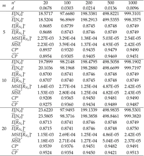
Table 10: Characteristics and simulated values of purely sequential procedure with

α=0.05,θ1=1,θ2=7,m=5, 10, 20 andR=0.875.

m n

∗

20 100 200 500 1000

d 0.0678 0.0303 0.0214 0.0136 0.0096

5

E[Nd]∗ 18.5717 97.6680 198.3381 498.8221 999.3101

b

E[Nd]∗ 18.5204 96.8969 198.2913 499.5355 998.3575 E[bR_Nd]∗ 0.8685 0.8739 0.8745 0.8748 0.8749 b

E[bRNd]∗ 0.8688 0.8743 0.8746 0.8749 0.8749 MSE[bRNd]

∗

2.27E-03 3.29E-04 1.38E-04 5.03E-05 2.54E-05 [

MSE∗ 2.23E-03 3.59E-04 1.37E-04 4.93E-05 2.42E-05

CP∗ 0.8937 0.9320 0.9435 0.9479 0.9490

c

CP∗ 0.8954 0.9305 0.9405 0.9469 0.9451

10

E[Nd]∗ 19.7899 98.2148 198.4795 498.5058 998.1902

b

E[Nd]∗ 20.1036 98.1968 198.2880 498.6699 999.7197 E[bRNd]∗ 0.8700 0.8741 0.8746 0.8748 0.8749

b

E[bR_Nd]∗ 0.8707 0.8740 0.8745 0.8748 0.8749

MSE[bRNd] ∗

1.64E-03 2.77E-04 1.25E-04 4.87E-05 2.42E-05 [

MSE∗ 1.53E-03 2.80E-04 1.25E-04 4.82E-05 2.43E-05

CP∗

0.9208 0.9365 0.9450 0.9481 0.9490 c

CP

∗

0.9275 0.9360 0.9434 0.9489 0.9487

20

E[Nd]∗ 23.6220 97.9493 199.1339 498.9835 998.5301

b

E[Nd]∗ 23.5805 98.3716 198.3858 498.8461 999.3820 E[bRNd]∗ 0.8713 0.8741 0.8746 0.8748 0.8749

b

E[bRNd]∗ 0.8715 0.8741 0.8746 0.8748 0.8750 MSE[bRNd]

∗

1.15E-03 2.69E-04 1.25E-04 4.86E-05 2.42E-05 [

MSE∗ 1.18E-03 2.71E-04 1.27E-04 5.04E-05 2.37E-05

CP∗

0.9539 0.9376 0.9451 0.9482 0.9491 c

CP∗ 0.9524 0.9354 0.9450 0.9421 0.9513

Table 11: Characteristic of the two-stage procedure and the smallest m such that coverage probability be at least 95%.

n∗

20 100 200 500 1000

θ1=1, θ2=2 _md 0.1377₁₆ 0.0616₈₈ 0.0616₁₈₁ 0.0275₄₆₄ 0.0195₉₃₉

E[Nm] 20.4368 100.6199 200.6407 500.5397 1000.3440

b

E[Nm] 20.4368 100.6246 200.6659 500.6219 1000.4066 E[bRNm] 0.6630 0.6659 0.6663 0.6665 0.6666 b

E[bR_Nm] 0.6631 0.6660 0.6663 0.6665 0.6666

MSE[bRNm] 5.00E-03 9.89E-04 5.00E-04 2.00E-04 9.88E-05

[

MSE 4.90E-03 9.91E-04 5.00E-04 2.00E-04 9.90E-05

CP 0.9505 0.9500 0.9500 0.9500 0.9500

c

CP 0.9507 0.9503 0.9493 0.9496 0.9495

θ1=1, θ2=3 d 0.1162 0.0520 0.0367 0.0232 0.0164

m 17 87 178 458 931

E[Nm] 21.7933 102.1451 202.1986 502.2104 1002.0449

b

E[Nm] 21.8044 102.1311 202.2000 502.1621 1001.9552 E[bRNm] 0.7455 0.7491 0.7495 0.7498 0.7499 b

E[bRNm] 0.7455 0.7490 0.7495 0.7498 0.7499

MSE[bRNm] 3.48E-03 7.03E-04 3.52E-04 1.41E-04 7.03E-05

[

MSE 3.48E-03 7.03E-04 3.53E-04 1.40E-04 7.06E-05

CP 0.9518 0.9501 0.9500 0.9500 0.9500

c

CP 0.9516 0.9491 0.9495 0.9501 0.9498

θ1=1, θ2=5 _md 0.0861₁₇ 0.0385₈₆ 0.0272₁₇₆ 0.0172₄₅₂ 0.0122₉₂₂

E[Nm] 23.3406 104.1099 204.3535 504.4301 1004.4449

b

E[Nm] 23.2954 104.1361 204.3072 504.3212 1004.7583 E[bR_Nm] 0.8290 0.8324 0.8329 0.8331 0.8332 b

E[bR_Nm] 0.8290 0.8325 0.8329 0.8331 0.8332

MSE[bRNm] 1.93E-03 3.86E-04 1.93E-04 7.72E-05 3.86E-05

[

MSE 1.93E-03 3.89E-04 1.93E-04 7.66E-05 3.86E-05

CP 0.9501 0.9500 0.9500 0.9500 0.9500

c

CP 0.9503 0.9496 0.9503 0.9508 0.9497

θ1=1, θ2=7 d 0.0678 0.0303 0.0214 0.0136 0.0096

m 17 86 175 450 917

E[Nm] 24.4921 104.1099 205.5915 505.8347 1005.8066

b

E[Nm] 24.5044 104.1459 205.5118 506.0394 1005.5856 E[bRNm] 0.8713 0.8324 0.8746 0.8748 0.8749 b

E[bRNm] 0.8713 0.8324 0.8746 0.8748 0.8749

MSE[bR_Nm] 1.18E-03 3.86E-04 1.20E-04 4.79E-05 2.40E-05 [

MSE 1.17E-03 3.84E-04 1.21E-04 4.78E-05 2.39E-05

CP 0.9513 0.9500 0.9500 0.9500 0.9500

c

CP 0.9517 0.9498 0.9490 0.9501 0.9501

6

Real Data

In this section, the analysis of a pair of real datasets is presented for illustrative purposes. Breaking strengths of jute fiber into two different gauge lengths are shown in Table 12-13. These two datasets were used by Xiaet al. (2009) and presented earlier in Mirjaliliet al. (2016). According to the latter, the data in Tables 12-13 have exponential distribution. Let random variables,XandYbe breaking strengths of jute fiber of gauge length 10mm and 20mm, respectively. Define reliability parameter under the stress-strength model, as the probability that jute fiber of gauge length 20 mm endures more than that of gauge length 10 mm.

Table 12: Dataset 1 (Breaking strength of jute fiber of gauge length 10 mm).

693.73 704.66 323.83 778.17 123.06 637.66 383.43 151.48 108.94 50.16 671.49 183.16 257.44 727.23 291.27 101.15 376.42 163.40 141.38 700.74 262.90 353.24 422.11 43.93 590.48 212.13 303.90 506.60 530.55 177.25

Table 13: Dataset 2 (Breaking strength of jute fiber of gauge length 20 mm).

71.46 419.02 284.64 585.57 456.60 113.85 187.85 688.16 662.66 45.58 578.62 756.70 594.29 166.49 99.72 707.36 765.14 187.13 145.96 350.70 547.44 116.99 375.81 581.60 119.86 48.01 200.16 36.75 244.53 83.55

Treating these two datasets as universal, we implemented both two-stage and purely sequential procedures, drawing observations (X,Y) from the full set of data as needed. To obtain the fixed-width 2dasymptotic confidence interval for parameterR, we carried out a single run under both procedures. Tables 14-15 provide the results derived from implementing the stopping rules from (3.1) and (4.1) respectively, when the initial sample size m =5, 10, α = 0.05 and d = 0.3, 0.2, 0.15 are chosen arbitrarily. Under both methodologies, the final estimators ˆRNmand ˆRNdtended to get closer to their exact value ˆR=0.482 obtained from the full data as the initial sample sizemincreases. Both estimators ˆRNm and ˆRNd are less than 0.5. It means that jute fibers of gauge length of 20 mm do not endure more than jute fibers of gauge length of 10 mm.

Table 14: An illustration with breaking strength of jute fiber of gauge length 10 mm, 20 mm, withd=0.3, 0.2, 0.15,m=5, 10 andα=0.05 using the two-stage procedure.

d m=5 m=10

0.3

Pilot Data:

X: 50.16, 108.94, 163.40, 376.42, 637.66 Y: 594.29, 113.85, 756.70, 36.75, 48.01,

¯

X5=418.976, ¯Y5=490.518

−→_Nm=₆

Second Stage Data Size: X:530.55

Y:662.66 ¯

XNm=418.976, ¯YNm=490.518

−→bR_Nm=0.5390

(bR_Nm−d,bR_Nm+d)=(0.239,0.839).

Pilot Data:

X: 727.23, 163.4, 637.66, 123.06, 50.16, 671.49, 353.24, 700.74, 212.13, 257.44 Y: 200.16, 145.96, 350.70, 578.62, 187.13, 756.70, 36.75, 375.81, 113.85, 166.49

¯

X10=389.655, ¯Y10=291.217

−→_Nm=10

Second Stage Data Size: Pilot Data is enough.

¯

XNm=389.655, ¯YNm=291.217

−→bR_Nm=0.4277

(bR_Nm−d,bR_Nm+d)=(0.1277,0.7277).

0.2

Pilot Data:

X: 303.90, 212.13, 291.27, 693.73, 383.43 Y: 116.99, 45.58, 581.60, 707.36, 119.86

¯

X5=376.892, ¯Y5=314.278

−→_Nm=₁₂

Second Stage Data Size:

X: 151.48, 727.23, 637.66, 353.24, 530.55, 177.25, 101.15

Y: 662.66, 375.81, 688.16, 145.96, 48.01, 284.64, 113.85

¯

XNm=380.2517, ¯YNm=324.2067

−→bR_Nm=0.4602

(bR_Nm−d,bR_Nm+d)=(0.2602,0.6602).

Pilot Data:

X: 212.13, 704.66, 727.23, 303.9, 530.55, 323.83, 123.06, 693.73, 141.38, 506.6 Y: 48.01, 581.60, 765.14, 244.53, 284.64, 116.99, 350.70, 662.66, 756.70, 113.85

¯

X10=426.707, ¯Y10=392.482

−→_Nm=₁₂

Second Stage Data Size: X: 506.60, 212.13 Y: 350.70, 116.99

¯

XNm=415.4833, ¯YNm=366.0425

−→bR_Nm=0.4684

(bR_Nm−d,bR_Nm+d)=(0.2684,0.6684).

0.15

Pilot Data:

X: 257.44, 323.83, 303.9, 506.6, 123.06 Y578.62, 166.49, 244.53, 36.75, 113.85,

¯

X5=302.966 , ¯Y5=228.048

−→_Nm=₂₁

Second Stage Data Size:

X: 530.55, 422.11, 323.83, 700.74, 123.06, 108.94, 183.16, 163.40, 590.48, 177.25, 778.17, 727.23, 101.15, 212.13, 50.16, 262.9

Y: 594.29, 113.85, 36.75, 145.96, 375.81, 187.85, 765.14, 547.44, 116.99, 419.02, 71.46, 662.66, 99.72, 581.60, 244.53, 48.01

¯

XNm=331.909, ¯YNm=292.92

−→bR_Nm=0.4688

(bR_Nm−d,bR_Nm+d)=(0.3188,0.6188).

Pilot Data:

X: 141.38, 530.55, 376.42, 353.24, 693.73, 637.66, 43.93, 291.27, 212.13, 383.43 Y119.86, 765.14, 350.70, 200.16, 375.81, 116.99, 662.66, 244.53, 707.36, 166.49

¯

X10=366.374, ¯Y10=370.97

−→_Nm=₂₂

Second Stage Data Size:

X: 506.60, 177.25, 43.93, 108.94, 183.16, 671.49, 353.24, 141.38, 727.23, 50.16, 778.17, 123.06

Y: 200.16, 45.58, 113.85, 594.29, 585.57, 71.46, 662.66, 419.02, 116.99, 166.49, 284.64, 48.01

¯

XNm=342.1977, ¯YNm=319.0191

−→bR_Nm=0.4825

(bR_Nm−d,bR_Nm+d)=(0.3325,0.6325).