A Preemptive multimode resource constrained project scheduling model with cash flows

(1)

A Preemptive multimode resource constrained project scheduling

model with cash flows

1

Soltani

Hassan

,

2

Hamta

Nima

,

* 1

Ehsanifar

Mohammad

1

Industrial Engineering Department, Arak Branch, Islamic Azad University, Arak, Iran Iran Arak, Technology, of

University Arak

Engineering, Mechanical

of Department 2

[email protected], [email protected], [email protected]

Abstract

Resource constrained project scheduling problem is one of the most important issues in project planning and management. The objective function of this problem is to minimize the completion time of a project. When there is budget constraint or high risk for investment, using the criteria such as cash flows is so important. The development of computer systems and processors makes it possible to take more assumptions into modeling to obtain robust optimal solution. Recent research has been conducted on multimode resource constrained project scheduling problem with preemptive activities (P-MRCPSP). Assuming preemption of activities causes the model to approach the real-world problems in project scheduling. This assumption may occur due to factors such as equipment failure and shortage of resources. In most of the previous studies, the change in mode of activities was not possible after the discontinuation. In this paper, it is assumed that each activity can continue in various modes of operation after a stop. The developed model aims to minimize project completion time and maximize cash flow of the project, simultaneously. Two algorithms, i.e. Simulated Annealing (SA) and Multiple Objective Particle Swarm Optimization (MOPSO) have been developed to solve the proposed model. The obtained results of these two algorithms show that SA algorithm has the better performance.

Keywords:

P-MRCPSP, cash flows, simulated annealing, non-dominated sorting genetic algorithm

1- Introduction

Resource constrained project scheduling problem (RCPSP) is one of the most important model in project scheduling (Hill et al. 2018). The assumption of the implementing activities in different modes of execution has been created (MRCPSP). In this case, the execution of activities in each executive mode requires a certain amount of resources, and also takes a certain amount of time. Kolisch and Sprecher (1997), Van Peteghem and Vanhoucke(2010), Hartmann and Briskorn (2010) and Mori and Tseng

(1997) have compared these two models. Previous studies have proven the advantage of the model MRCPSP to RCPSP (De Reyck and Herroelen, 1999).

RCPSP has been of two respects to researchers; the First one is the applicability of these models in project management and the variety of constraints and goals of decision makers. The second one is that these problems are NP-hard that have led researchers to solve such problems by using various methods, such as Meta-heuristic algorithms (Blazewicz et al. 1983).

P-MRCPSP is a branch of MRCPSP in that each activity can be disconnected at specific times until completion of the activity. In the literature review about (P-MRCPSP), any activity after the termination should be followed in the same previous execution mode.

*Corresponding author

Journal of Industrial and Systems Engineering

Vol. 12, Special issue on Project Management and Control, pp. 28-44 Winter (January) 2019

(2)

This limitation is set to prevent an increase in the calculation of the change in execution mode.

Many studies have shown the superiority of the model (P-MRCPSP) to (MRCPSP) (Van Peteghem and

Vanhoucke, 2010), (Hartmann and Briskorn ,2010) and (Damak et al. 2009).

Russell was the first one who considered the scheduling of the project with the goal of maximizing net present value (NPV) (Russell , 1980). His model considered only the preconditions. Russell transforms the nonlinear model into a linear model using the Taylor series approximation. Grinold (1972) added the time-limit for the project to Russell's model and solved it using two different algorithms.

Buddhakulsomsiri and Kim (2006) presented a mathematical model for the P-MRCPSP problem and then solved the proposed model by branching and boundary method. The results of this study showed that the completion time of the project in the P-MRCPSP problem is less than that of the

MRCPSP. Van Peteghem and Vanhoucke (2010) solved the problem of resource constraints project

scheduling within two modes of preemptive and non-preemptive activities with a genetic algorithm

based on two populations.The results of this study showed that the solutions from the P-MRCPSP

model are closer to the optimal solution than the MRCPSP, but the solving time in the preemptive model increases dramatically.

The changing ability of executive mode after the preempted of activities was first considered by Afshar Najafi (2014). He called this proposed model (P-MRCPSP-MC) whereas MC means Mode Changeability. Although the model provided by him greatly increased the resolution time, the model's performance minimized the completion time of the project and increased freedom to select the appropriate executive mode that led to the leveling of resources;the assumption of the change in the mode of operation really justifies the activities well.

In this paper, by adding the objective function of maximizing net cash flow to the model provided by Afshar Najafi (2014) and making profitable changes in the model, it attempts to change the mode of operation of activities to bring the model closer to real problems.Paying a certain percentage to the contractor after the completion of a certain phase of the project will give him enough incentive to maximize the cash flow of the project by changing the mode of execution of the activities.

2- Problem definition

The given assumption is N activity, which is represented by an AON grid graph as a graph of G= (N, A). In this graph, the nodes represent activities and arcs indicating the pre-existing relationships of activities. Activities are numbered from 1 to n and should be assigned to any activity, renewable resources, and non-renewable resources. For each sub activity, a fixed task is presented, as in the DTRTP models, which basically shows how much work should be done. Each sub activity can be done in each of the different modes of operation. For example, with different speeds and resource requirements as long as the content of the work is met.

Performing an activity can temporarily stop at discrete times and restart in another state or same state again. We show the progress of activity i in the mode of m_iwith

i

im

W . In order to advance each

activity in any execution mode, we need the renewable (Rρ) and non-renewable (

R

γ) resources listed for that (a ) of each renewable resource and (ρ_k a ) of any non-renewable resource. _lγ

2-1- Model assumptions

The purpose of this model is to provide a practical program for predicting the exact planning of a project. The objectives are to minimize the completion time of the project and maximize net cash flow.To achieve this, it is necessary to identify the modes of operation for activities. The assumptions of the problem are as follows:

1. Activities have a predetermined relationship.

2. Each activity is required from the end of its pre-activity.

3. Stop at any activity after the start and after a certain amount of work is allowed. 4. Every activity takes place at the earliest start time to the latest end time.

5. The prerequisite relationships are only the end to the start.

6. The first and final activity is hypothetical and has come to facilitate formulation. 7. Activities are not delayed or prepared.

(3)

8. Resources with limited capacity and a certain amount.

9. Each activity, depending on the chosen mode of operation, needs a certain amount of renewable and non-renewable resources.

10. The budget is not limited.

11. Time of payments to the contractor and costs by the contractor from the beginning of the project. 12. Every activity uses one or more sources.

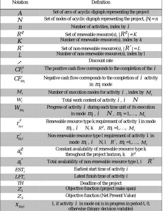
2-2- Parameters and decision variables

The notations and definitions related to the parameters and decision variables for the formulation of the mathematical model are as follows.

Table 1. Notations, parameters and decision variables

Notation Definition

A

Set of arcs of acyclic digraph representing the project

N

Set of nodes of acyclic digraph representing the project, |N| = n

n

Number of activities, index by

i

R

ρ Set of renewable resource(s), |

R

ρ| = K

K

Number of renewable resource(s), index by k

R

γ Set of non-renewable resource(s), |

R

γ| = L

L

Number of non-renewable resource(s), index by l

α Discount rate

i

CF

+ The positive cash flow corresponds to the completion of the

i

-i

im

CF

Negative cash flow corresponds to the completion of

i

activity in

m

_i mode

i

M Number of execution modes for activity

i

, index by i

M

i

W Total work content of activity

i

,

i

∈

N

i

im

W

Progress of activity

i

during each time unit of its execution in mode

m

_i ,

i

∈

N

,

m

_i = 1,. . ., M_i im ki

r

ρ Renewable resource type k requirement of activity

i

in mode

i

m

,

i

∈ N, k ∈Rρ,

m

_i =1,. . ., M_i i

im l

r

γ Non-renewable resource type l requirement of activity

i

in mode

m

_i,

i

∈ N, l ∈Rγ,

m

_i =1,. . ., M_i

k

a

ρ Constant availability of renewable resource type k

throughout the project horizon, k ∈ Rρ l

a

γ Total availability of non-renewable resource type l, l ∈

R

γ

i

EST Earliest start time of activity i i

LFT Latest finish time of activity i

TH Deadline of the project

1

Z Objective function (project make span) 2

Z Objective function (Net Present Value)

i

im t

x

1, if activity

i

in mode mi is in progress in period t, 0, otherwise (binary decision variable)

In the formulation provided, t is defined only in the interval. By using the defined notations, the mathematical model is presented as follows.

(4)

2-3-Mathematical model

This problem can be formulated with two objectives, i.e. minimizing project completion time and maximizing the cash flows of the project:

1 1 . n n n LFT nm t EST

Min Z t x

+

=

∑

(1)

-2

1 1 1 1

(1

)

.

(1

)

n i i i i n i LFT M n n im T

i t im t

i i EST m

CF

Max Z

CF

α

x

α

+

= = + =

=

+

−

+

∑

∑ ∑ ∑

(2)

1 1 . n i i i n i LFT M

im im t i EST m

w x w i N

+ =

≥ ∀ ∈

∑ ∑

(3)

[

]

1

1 , 1,

i i i

M

im t i i

m

x i N t EST LFT

=

≤ ∀ ∈ ∀ ∈ +

∑

(4)

( )1

1 ,

[

1,

1 ,

]

i i

im t im t i i i i

x

+

x

_{′ +}

≤ ∀ ∈

i

N

∀ ∈

t

EST

+

LFT

−

∀

m

≠

m

′

(5)

(

)

[

]

( 1)

1 1

. , , 1, 1

j

n i

i i j

i j

M

LFT M

im im t i jm t i i

TH m m

w x w x ₊ i j A t EST LFT

= =

≥ ∀ ∈ ∀ ∈ + −

∑ ∑

∑

(6)

1 1

. , 1,...,

i

im ki i i

M n

im t k i m

rρ x aρ k Rρ t TH

= =

≤ ∀ ∈ =

∑ ∑

(7)

1 1 1

. i i i i i i M LFT n

im l im t l i m t EST

rγ x aγ l Rγ

= = = +

≤ ∀ ∈

∑ ∑ ∑

(8)

[

]

0,1

,

1,

,

1,...,

i

im t i i i i

x

=

∀ ∈

i

N

∀ ∈

t

EST

+

LFT

m

=

M

(9)

The first objective function (1) monitors the completion time of the project. The second objective function (2) has two parts, which shows the first part of the positive cash flows of the project and the second part of the negative cash flows of the project, while this function follows the purpose of maximizing cash flows.Limit (3) ensures that the content of the work of each activity is fulfilled. Limitation (4) states that each activity can only be in one state at any time. Limitation (5) prohibits the switching of an executable without interrupting activity. In the constraint (6), preconditions have been considered.Limits (7) and (8) ensure that the limitations of renewable and non-renewable resources are met, and finally, the constraint (9) shows the decision variable.

There are plenty of ways to pay for scheduling a project with regard to the planners' objectives and type of project: payment at equal intervals, payment after completion of predetermined stages, payment at the end of the project, and so on.In the introduced model, payments are considered at the end of each phase of the project. This method of payment is very common because of the high flexibility in the audit, monitoring, and portfolio selection of contractors.

3- Solution method

3-1- Simulated annealing algorithm

Simulated Annealing (SA) is a Monte Carlo model approach. This method acts on the basis of atomic structure, entropy, and temperature during the refrigeration of a material, and is one of the most effective meta-heuristic algorithms for solving optimization problems.The simulated annealing algorithm was first introduced by Kirkpatrick and Vecchi (1983). The algorithm assumes that the

material is present in the molten state, and its temperature slowly decreases every moment. The

material reaches the thermal equilibrium at any temperature and its energy is minimized. In this algorithm, the temperature considered as a control parameter and play important role in preventing that falling into the optimal local response.

(5)

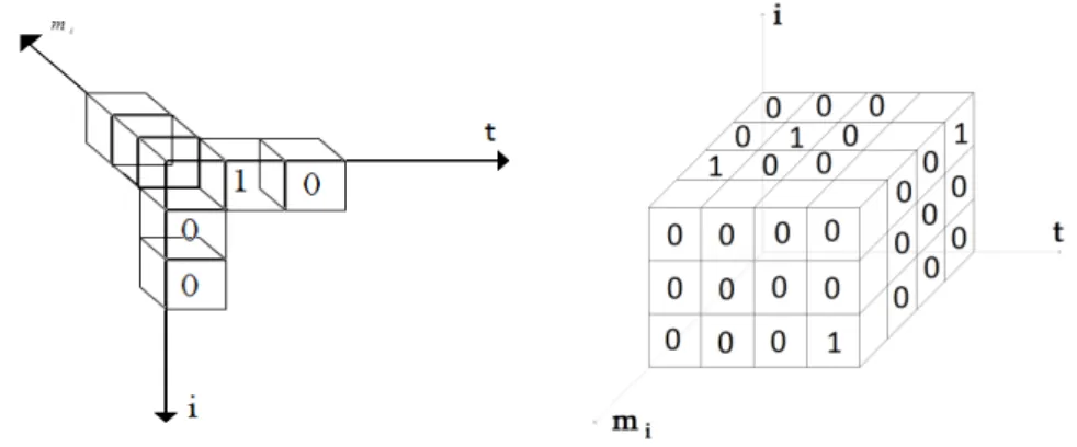
3-1-1- Structure of Solutions

The structure of the solution actually represents the space of the problem and its introduction in all of the meta- heuristic algorithms is important and necessary. In the two-objective model, each of the responses presented indicates that each sub-activity in which execution mode is executed. So for each activity, you can consider a three-dimensional matrix so that if sub activity

i

is executed at time t in the mode m_iis 1, otherwise it is 0.

Each activity has its own three dimensional matrix that shows the structure of the failures and the completion time of the activity.

Fig 1. Demonstration of a solution

3-1-2- Generating the initial solution

The proposed algorithm first takes the executive mode of all activities into account so that the project resource constraints are not violated.For this, the algorithm for any activity, regardless of its execution time, considers the state of execution to be the least use of resources, and then completes the three dimensional matrices of activities according to the existing pre-existing relationship. If there is not a prioritized relationship between several activities, one of the activities will be randomly selected.

3-1-3- Neighborhood mechanism

To create a neighborhood for a solution, the operating mode algorithm changes each of the following activities. This is done so that in every 3D matrix everywhere under the activity

i

was set to 1, instead of 0, it activates without changing the vector of the row and column in the other executable mode.

3-1-4- Selection of Initial Temperature

Determining the initial temperature is one of the important parameters in the convergence to the optimal solution. For the first time, Abramson used the average cost of the system to equal the standard deviation of the cost of the system (Abramson et al. 1999). Due to the efficiency of the initial temperature determination method provided by Abramson and the use of this method in various studies of standard deviation, the random model of the objective functions of the problem is obtained as follows.

Sample average = 1

( )

1

NSA MP

j

Obj j

M

NSA MP

=

−

∑

₍₁₀₎

Sample standard deviation

2 1

( ( ) )

1

NSA MP

j

Obj j M

NSA MP

=

− =

−

∑

₍₁₁₎

0

(

/

1)

T

=

Sqrt Sum NSA MP

−

(12)

(6)

Due to the convergence rate of the algorithm and the obtained results, the initial temperature of the algorithm can be entered manually.

3-1-5- Temperature reduction mechanism

The function of decreasing the temperature and moving the algorithm toward an optimal solution requires a relation that is considered as follows:

1

(

)

1, 2,...,

i i

T

=

α

T

₋

∀ =

i

n

(13)

[

In the above relation, the temperature reduction coefficient is considered to be between 0.5 and 0.99 in most studies. The proposed algorithm can be set up. Also, this mechanism is provided for the frequency of decreasing temperature (n).

3-1-6- Markov chain length

In this paper, due to the importance of finding the optimal and accurate solution in the problem space, the number of points examined by the algorithm is obtained through the Markov chain. Selection of Markov chain length is possible in a variety of ways.In this study, the length of the chain (

L

_n) is considered according to the size of each activity. Of course, in the algorithm provided for each activity, there is the ability to enter the value of

L

_n manually and according to the length of the activity.

3-1-7- The mechanism for accepting the solution

How to accept the solution is one of the important factors in convergence to the optimal solution. At this stage, suppose that the solution A leads to the value of the Z-objective function, and considers the neighborhood mechanism of solving A 'with the value of the objective function Z' of the candidate of comparison with A.In this case, if ΔZ = Z - Z' (maximization problem).

1. If ΔZ is smaller than zero, it will be improved in the value of the function, and as a result, the neighbor solution A' will be replaced by the solution A, and the optimal objective function will be equal to Z'.

2. If ΔZ is greater than zero, then the value of the objective function is not recovered. In this case, the value of EXP (-ΔZ / t) is compared with a random number between 0 and 1. If the random number is bigger, the neighborhood solution replaces the current solution. Otherwise the neighborhood solution is not accepted and creates another neighborhood solution.

3-1-8- Pseudo-code of simulated annealing algorithm

The pseudo-code of the algorithm for the proposed model is developed as follows:

Parameter setting: Popsize, iteration, num.struct, Archsize, T, B Initialization: generate initial solutions

Evaluation: evaluate initial solution

Perform non-dominated sorting and calculate ranks Calculate crowding distance (CD)

Sort population according to ranks and CDs t

P

= P:population For it=1:iteration

For i=1:popsize For j=1:num.struct

t

S

(i)= perform neighborhood structure on the solution i of the population

P

_t (i) End

End

Perform non-dominated sorting and calculate ranks (

S

_t) Calculate crowding distance (CD) (

S

_t)

(7)

Sort population according to ranks and CDs (

S

_t ) For i= 1:popsize

If dominates (

S

_t (i).

P

_t (i))

1

t

P

₊ (i)=

S

_t (i) Else

P = exp i i

f

T

−∆

If rand < P t

Q

(i)=

S

_t (i) End End

End End

0

t t t

A

=

P

∪

A T

R

_t) Calculate crowding distance (CD) (

R

_t)

Sort population according to ranks and CDs (

R

_t) P,= choose popsize number of the solution of the

R

_t

t t t

A

=

P

∪

A

_t ) Calculate crowding distance (CD) (

A

_t)

If size of

A

_t > Archsize t

A

= select frontmax number of the solution Else

Update T (T = α ×

T

0)

end

3-2- MOPSO algorithm

The MOPSO algorithm uses PSO operators. Coello et al. Introduced this algorithm in 2002 and developed it in 2004 and 2006 (Coello et al. 2007). In this algorithm, the best non-dominated solutions are stored in an external memory. The general structure of the algorithm is as follows: For each particle in the population, the position of the current particle is randomly initialized. Initialize the current particle velocity or equate it with zero. Consider the best position (the best local position) of the current particle with the current position.By using the fitness function, evaluate the fitness of each of the particles in the population and consider the best position among them to be the best in the world. Until the convergence conditions are met, update the current particle size for each particle in the population. Update the current particle status.Assess the fitness of the current particle using the fitness function. Update your best position (best local position) of the current particle. Update your best overall position.

The pseudo-code of the multiple objective particle swarm optimization algorithm for the suggested model is as follows. The process of updating the values of the velocity and position of particles in both of the main loops of the algorithm is performed.In addition, the Repository collection is updated by using the concept of overcoming in repetitive repetitions, and the best front of the Repository is the output of the algorithm.

(8)

Begin

Input n-Particle, C1, C2, W and Max-iteration Generate initial particles

Evaluate fitness values of the initial particles Create the best personal memory

Create the best global memory

Create grid index for solution dimension Find repository member

For it=1: Max-iteration do For j=1: n-Particle do Select the leader particle Update particle position

Evaluate particle's fitness value

Apply mutation and update particle position Update the best personal memory

Update the best global memory End For

Find repository members

Combine new repository member with repository member 𝑟𝑟𝑒𝑒𝑝𝑝=𝑅𝑅𝑒𝑒𝑝𝑝⋃𝑅𝑅𝑒𝑒𝑝𝑝𝑛𝑛𝑒𝑒𝑤𝑤 Update repository member using the dominance Sorting algorithm

Delete extra repository members End For

Output: extract repository front End

Due to need for a feasible solution, it is necessary to store the soluble structure according to a specific structure that responds to this structure as a demonstration. The production of the initial solution to the problem of project scheduling is called the scheduling method. This method plays a very important role in most meta-heuristic algorithm and problem solving methods.The method of representation of the solution in this solution, in random numbers in the range of zero and one, is in two rows. The length of these rows is equal to the total time of the operations, the first line is related to the assignment of the state of execution, and the second line is related to the activities.

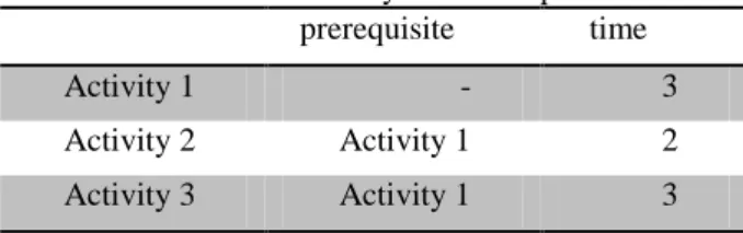
The following example is presented to illustrate the best methodology, displaying the solution and decoding it.Suppose we have a problem with three activities and three executive modes, respectively, given in table 1. According to the example data, total activity time is equal to 8.So the method of displaying the solution to this problem is in two rows of length 8 and is presented in figure 1. To determine the optimal modes of doing any activity, first, the number of activities from the first line of the solution method is selected. These numbers are multiplied by the number of executable modes of each activity and they are rounded upwards.The resulting numbers represent the operating modes of the activity. This process is schematically shown in figure 2.

0.740 0.220

0.390 0.130

0.520 0.030

0.630 0.870

V1

0.430 0.090

0.970 0.640

0.160 0.800

0.310 0.510

V2

Fig 2. The method of displaying numbers numerically between zero and one

Table 2. Primary data example time prerequisite

3

-Activity 1

2 Activity 1

Activity 2

3 Activity 1

Activity 3

(9)

Fig 3. Select execution modes example

Since activity interruptions are allowed, the method of displaying the solution must be discrete so that, in order to determine the sequence of the tasks, each activity is divided according to the time that those activities are performed, and for each activity a separate section is considered. At this stage, for each part, a set is defined as activity.In this set, there are defined activities that have an empty set of prefixes. Then at each step the numbers in the second layer of figure 1 are multiplied by the number of elements of the activity set, and the resulting numbers are directed to the top, and the nth member of the activity set is assigned.If all the parts of an activity are assigned, it should be considered as part of the assigned activities. This process continues until the last part of an activity is allocated. Figure 3 shows that activities should be performed in modes 3, 3 and 1, respectively. This response structure has been implemented for both MOPSO and SA algorithms.

Fig 4. Select execution modes

4-Computational results

4-1- Generating sample problem

Since the model presented in this paper for the first time considers activities in a preemptive mode and changes the mode of operation after discontinuation of activity, using sample problems in the PSP Lab library or problems that is generated by Pro Gen software does not evaluate and compare proposed algorithms due to the difference in the structure of the problems. Therefore, the problem with 9 activities that the content of all activities is randomly generated is designed to examine proposed algorithms.

Fig. 5. Precedence network of a problem

1

2 5

3

4 8

9 6

7

0.870 0.630 0.030 3 3 1

0.030 0.520 0.130 0.390 0.220 0.740 0.870 0.630

1 2 1 1 1 3

3 2

(10)

Table 3. Generated random problem i γ im l

r

ρ

im k_i

r

i im

W

i M Mode i W

Number of activity

0 0 1 1 1 1 5 23 3 1 17 2 13 11 2 2 7 15 5 1 13 3 11 8 3 2 13 9 4 1 11 4 11 13 6 2 10 12 7 1 5 5 9 12 5 2 13 17 3 1 14 6 9 11 2 2 8 10 5 1 22 7 12 15 3 2 10 9 6 1 9 8 8 3 3 2 0 0 1 1 1 9

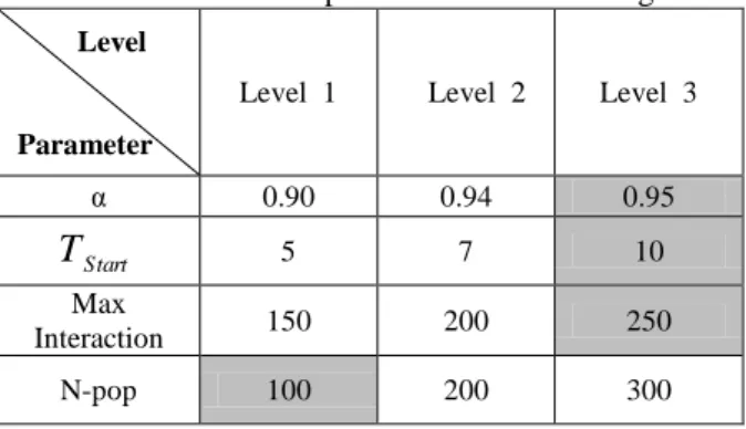
4-2- Set parameters

The effectiveness of meta-heuristic algorithms is highly dependent on the values of its parameters. Many methods have been used to set the parameter in previous studies, including factorial, orthogonal array and Taguchi experimental design.In Taguchi method, after determining the effective factors on the solution, different levels are considered for these factors. After examining the algorithm's solutions for these values, a surface is selected that has the lowest number of signal to noise.Table 3 shows the levels of effective factors in the SA algorithm and in table 4, the levels related to the effective factors in the MOPSO algorithm. Given the pseudo-codes of the two proposed algorithms and the number of effective parameters in the convergence of algorithms for the MPS algorithm from the L16 (5 factor and in 4 levels) array, and for the algorithm three of the L9 (4 factor and in 3 levels) array to adjust the parameters are used.

Table 4. Levels of the parameters of the SA algorithm

Level 3 Level 2

Level 1

Level Parameter 0.95 0.94 0.90 α 10 7 5 Start

T

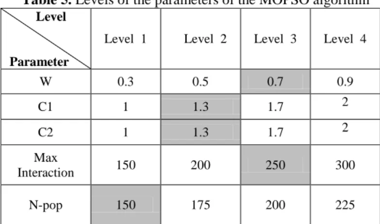
250 200 150 Max Interaction 300 200 100 N-pop 37

(11)

Table 5. Levels of the parameters of the MOPSO algorithm

Level 4 Level 3

Level 2 Level 1

Level

Parameter

0.9 0.7

0.5 0.3

W

2 1.7

1.3 1

C1

2 1.7

1.3 1

C2

300 250

200 150

Max Interaction

225 200

175 150

N-pop

Figures 6 and 7 show the noise signal diagram of the parameters used in the two proposed algorithms, which shows the optimal levels for each of the parameters.

Fig 6. Main Effects Plot for SN ratios (SA)

Fig 7. Main effects plot for SN ratios (MOPSO)

3 2 1 31

30

29

28

27

26

25

24

3 2

1 1 2 3 1 2 3

α

M

e

a

n

o

f

S

N

r

a

ti

o

s

T-start Max-interaction N-pop

Signal-to-noise: Smaller is better

4 3 2 1 30

29

28

27

26

25

4 3 2

1 1 2 3 4 1 2 3 4 1 2 3 4

C1

M

e

a

n

o

f

S

N

r

a

ti

o

s

C2 W N-pop Max-interaction

Signal-to-noise: Smaller is better

(12)

After solving designed experiments for both algorithms, the best level of these parameters in the SA algorithm for the Max-interaction parameter, 3 is obtained for the parameter

T

_Start level 3 for the parameter α level 3 and for the parameter N-pop level 1. In the MOPSO algorithm has the best level for W level 3, for the parameter C1 level 2, for the C2 parameter of level 2, for the N-pop parameter of level 1 and obtained for the Max-interaction parameter of level 3.

Table 6. Parameters of the MOPSO algorithm

Response Max-interaction N-pop W C2 C1 Run order 0.035 1 1 1 1 1 1 0.032 2 2 2 2 1 2 0.042 3 3 3 3 1 3 0.019 4 4 4 4 1 4 0.057 4 3 2 1 2 5 0.067 3 4 1 2 2 6 0.056 2 1 4 3 2 7 0.034 1 2 3 4 2 8 0.073 2 4 3 1 3 9 0.048 1 3 4 2 3 10 0.023 4 2 1 3 3 11 0.072 3 1 2 4 3 12 0.038 3 2 4 1 4 13 0.065 4 1 3 2 4 14 0.024 1 4 2 3 4 15 0.048 2 3 1 4 4 16

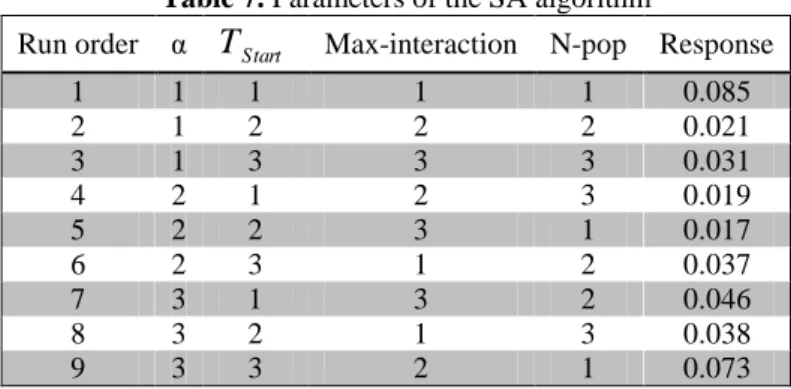
Table 7. Parameters of the SA algorithm

Response N-pop Max-interaction Start

T

α Run order 0.085 1 1 1 1 1 0.021 2 2 2 1 2 0.031 3 3 3 1 3 0.019 3 2 1 2 4 0.017 1 3 2 2 5 0.037 2 1 3 2 6 0.046 2 3 1 3 7 0.038 3 1 2 3 8 0.073 1 2 3 3 9

4-3- Computational results

In this section, the performance of proposed algorithms is investigated based on various indicators. By plotting the values of the indexes obtained from tables 5 and 6 as a graph and comparing algorithm index charts, it is shown that the SA algorithm performs better than MOPSO algorithm in terms of NPS, MS, SNS and RAS criteria. While the MOPSO algorithm performs better than the SA algorithm in terms of MID and Spacing metrics.

4-3-1- The mean ideal distance graph

The Mean Ideal Distance (MID) is the important criteria in the literature for evaluating Pareto solutions in multi-objective optimization. It is a simple metric that measures the mean distance from the ideal point. This criterion is usually used in optimization problems at which the ideal point for all of the objective functions is the (0, 0).

(13)

Fig 8. Comparison diagram of the MID index

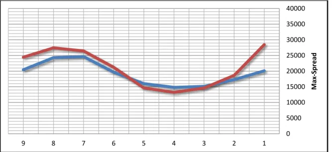
4-3-2- The Max-Spread graph

One of the most reputed criteria in the literature for evaluating Pareto solutions in multi-objectives optimization is the Max-Spread of optimal solutions (MS). This metric compares the dispersion of algorithmic responses and usually used to compare the results obtained from two-objective algorithms.

Fig 9. Comparison of the Max-Spread Index

4-3-3- Span of non-dominant solution graph

The proximity of algorithmic recursive responses is another criterion for evaluating Pareto solutions for multi-objective optimization. The Span of Non-dominant Solution (SNS) is a simple metric that measures the distance of optimal solutions from recursive responses.

1 2

3 4

5 6

7 8

9

SA 1.2 1.4 1 1.6 1.2 2 1.1 1.2 2

MOPSO 1.3 1.4 1.3 1.2 2.3 3.2 2 1.4 1.8

1 10

M

ID

0 5000 10000 15000 20000 25000 30000 35000 40000

1 2

3 4

5 6

7 8

9

M

ax

-S

pre

ad

(14)

Fig 10. Comparison diagram of the SNS index

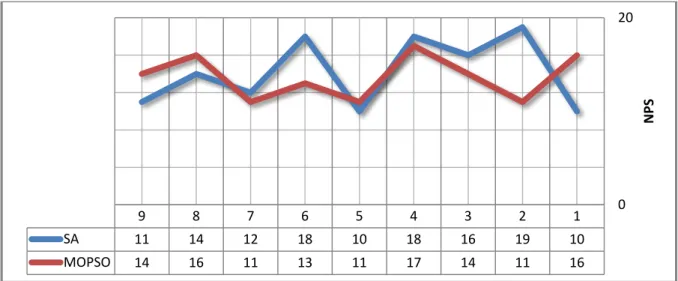
4-3-4- The number of Pareto solutions graph

The number of solutions received from each algorithm can be another suitable benchmark for

comparing algorithms. The number of Pareto solutions (NPS) is also given below to examine the

efficiency of the two algorithms used in this study.

Fig 11. Comparison diagram of the NPS index

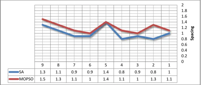
4-3-5-Spacing metric graph

The calculation of the uniformity of the spreading of non-dominant solution is another indicator that identifies the density of the responses obtained from the algorithms. The importance of this graph is to show the utility of the algorithm's solutions in pre-optimal replays.

0 20000 40000 60000 80000 100000

1 2

3 4

5 6

7 8

9

SN

S

1 2

3 4

5 6

7 8

9

SA 11 14 12 18 10 18 16 19 10

MOPSO 14 16 11 13 11 17 14 11 16

0 20

N

PS

(15)

Fig 12. Comparison of the spacing index

4-3-6- The Rate of Achievement to Objectives Simultaneously graph

One of the most commonly used indicators for comparing two-objective models is the Rate of Achievement to Objectives Simultaneously in achieving each goal (RAS).This indicator is important to show how much each of the algorithms has succeeded in meeting the desired goals.

Fig 13. Comparison diagram of the RAS index

Based on presented graphs and statistical analysis, the obtained results are as follows:

1. The proposed model maximizes the cash flow of the project and minimizes the completion time of the project simultaneously for the implementation of all phases of project.

2. The results obtained from the solution of the model by the proposed algorithms show that both algorithms yield similar results. Of course, the performance of the SA algorithm in the key indexes shows relative superiority to the MOPSO algorithm.

3. The proposed model can be considered as the appropriate basis for allocating funds to real projects.

5- Conclusions and suggestions for future studies

Scheduling is one of the most important components of project management. Despite the

development of specialized scheduling software, the unique constraints in the resources of each project have made planners to pay attention to RCPSP as their only option to achieve a

1 2

3 4

5 6

7 8

9

SA 1.3 1.1 0.9 0.9 1.4 0.8 0.9 0.8 1

MOPSO 1.5 1.3 1.1 1 1.4 1.1 1 1.3 1.1

0 0.2 0.4 0.6 0.8 1 1.2 1.4 1.6 1.8 2

Sp

ac

in

g

1 2

3 4

5 6

7 8

9

SA 0.7 0.55 0.5 0.6 0.5 0.55 0.6 0.6 0.7

MOPSO 0.6 0.55 0.5 0.5 0.4 0.5 0.5 0.6 0.5

0 0.1 0.2 0.3 0.4 0.5 0.6 0.7 0.8

RA

S

(16)

comprehensive plan. In this paper, a new mathematical model for the resource constraints project scheduling problem has been expanded and two algorithms, i.e. SA and MOPSO have been developed to solve this model.

The model presented in this paper aims to perform activities under different executive modes. The proposed model can be considered as scenario-based and under different time windows (with different execution times in each time window for each activity).Some parameters of the proposed model can also be considered in the uncertainty mode. The development of other meta-heuristic algorithms such as PSO and DEA algorithms to solve the presented model in this paper can also be useful suggestion for researchers in future studies.

References

Abramson, D., Krishnamoorthy, M., & Dang, H. (1999). Simulated annealing cooling schedules for

the school timetabling problem. Asia Pacific Journal of Operational Research, 16, 1-22.

Afshar-Nadjafi, B. (2018). A solution procedure for preemptive multi-mode project scheduling

problem with mode changeability to resumption. Applied Computing and Informatics, 14(2), 192-201.

Blazewicz, J., Lenstra, J. K., & Kan, A. R. (1983). Scheduling subject to resource constraints:

classification and complexity. Discrete applied mathematics, 5(1), 11-24.

Buddhakulsomsiri, J., & Kim, D. S. (2006). Properties of multi-mode resource-constrained project

scheduling problems with resource vacations and activity splitting. European Journal of Operational

Research, 175(1), 279-295.

Coello, C. A. C., Lamont, G. B., & Van Veldhuizen, D. A. (2007). Evolutionary algorithms for

solving multi-objective problems (Vol. 5). New York: Springer.

Damak, N., Jarboui, B., Siarry, P., & Loukil, T. (2009). Differential evolution for solving multi-mode

resource-constrained project scheduling problems. Computers & Operations Research, 36(9),

2653-2659.

De Reyck, B., & Herroelen, W. (1999). The multi-mode resource-constrained project scheduling

problem with generalized precedence relations. European Journal of Operational Research, 119(2),

538-556.

Grinold, R. C. (1972). The payment scheduling problem. Naval Research Logistics Quarterly, 19(1),

123-136.

Hartmann, S., & Briskorn, D. (2010). A survey of variants and extensions of the resource-constrained

project scheduling problem. European Journal of operational research, 207(1), 1-14.

Hill, A., Lalla-Ruiz, E., Voß, S., & Goycoolea, M. (2018). A multi-mode resource-constrained project

scheduling reformulation for the waterway ship scheduling problem. Journal of scheduling, 1-10.

Kirkpatrick Jr, S. CDG, and Vecchi, MP (1983). Optimizing by simulated annealing. Science,

671-680.

Kolisch, R., & Sprecher, A. (1997). PSPLIB-a project scheduling problem library: OR

software-ORSEP operations research software exchange program. European journal of operational

research, 96(1), 205-216.

Mori, M., & Tseng, C. C. (1997). A genetic algorithm for multi-mode resource constrained project

scheduling problem. European Journal of Operational Research, 100(1), 134-141.

Russell, A. H. (1970). Cash flows in networks. Management Science, 16(5), 357-373.

(17)

Van Peteghem, V., & Vanhoucke, M. (2010). A genetic algorithm for the preemptive and

non-preemptive multi-mode resource-constrained project scheduling problem. European Journal of

Operational Research, 201(2), 409-418.