Applying an Imperialist competitive algorithm for scheduling parts in a green cellular manufacturing system with consideration of production planning

(1)

226

Applying an Imperialist competitive algorithm for scheduling

parts in a green cellular manufacturing system with consideration

of production planning

2

Moghaddam

-, and Reza Tavakkoli

* 1

, Vahidreza Ghezavati

1

Hossein Raoofpanah

School of Industrial Engineering, South Tehran Branch, Islamic Azad University, Tehran, Iran

1

of Industrial Engineering, College of Engineering, University of Tehran, Tehran, Iran School

2

[email protected], [email protected], [email protected]

Abstract

A Cellular Manufacturing System (CMS) is the practical use of Group Technology (GP) in a production environment, which has received attention from researchers in recent years. In this paper, a mathematical model for the design of a cell production system is presented with consideration of Production Planning (PP). Consideration of environmental factors such as energy consumption and waste generated by machines in the proposed model is considered. Also, the problem of scheduling component processing in the presented model has been considered. Due to the complexity of the model presented in this paper, a hierarchical approach is proposed for solving the model. At first, the proposed model is analyzed without considering the scheduling topic using the GAMS software and the results are analyzed. Then an Imperialist Competitive Algorithm (ICA) was used to solve the scheduling problem. To evaluate the performance of the proposed model, numerical examples are used in small, medium, and large dimensions. In addition, the ICA presented in this paper is compared with the methods available in the literature as well as the genetic algorithm and its quality is confirmed.

Keywords: Cellular Manufacturing System, environmental effects, Imperialist Competitive Algorithm, machine-part processing scheduling.

1- Introduction

A Cellular Manufacturing System (CMS) usually used in different industrial plants to provide an efficient production system. Considering part scheduling in presence of environmental effects in this problem is a new challenge for researchers. These issues are not investigated deeply in the literature based on reviewed papers. Moreover, because of the complexity in problem-solving in a CMS, an optimal solution approach should be taken into account to find efficient solutions in reasonable computational time. In this section after reviewing some recent papers in this regard, a research gap will be identified and highlighted.

Wu et al. (2010) present an integrated model of facility transfer and production planning in dynamic cellular manufacturing based supply chain. On one hand, transferring facilities to the factory with large orders are investigated in their research. Chang et al. (2013) presented a bi-level mathematical model for solving Cell Formation Problem (CFP) and layout design. Mahdavi et al. (2013) developed a mathematical model so as to solve CFP and Cell Layout Problem (CLP), simultaneously. In their model, both intercellular and intracellular layout was determined. Rafiei and

*Corresponding author

Journal of Industrial and Systems Engineering

Vol. 12, No. 3, pp. 226- 248 Summer (July) 2019

(2)

227

Ghodsi (2013) presented a bi-objective model to solve CFP and operator assignment simultaneously. Satuglu and Suresh (2009) developed a goal programming model for cellular manufacturing problem. Wu et al. (2016) proposed a mathematical model in order to solve a dynamic cellular manufacturing problem considering operator assignment to machines. Tavakkoli-Mogaddam et al. (2010) considered a group fclea problem for CMS. Krishnahn et al. (2012) proposed a solution approach for CMS, where their model solved CFP and CLP simultaneously. Also, Bagheri and Bashiri (2014) presented a mathematical model for simultaneous solving CFP and CLP. Their objective was to minimize production and operators’ assignment costs to the machine in CMS. Jolai et al. (2012) proposed a mathematical model for handling CFP and its layout which was an extension of Wu et al. (2007) model in 2007. This problem dealt with CFP and its layout concurrently.

Geary et al. (2018) considered a scheduling and communication process to maximize processing availability by generating real-time data about lab space, technologist, and equipment utilization. Darussalam et al. (2015) presented an analytical effort for saving energy in a machine shop environment by optimizing the assignment of manufacturing processes to various machines and grouping machines in various cells for minimizing parts transportation distance. A nonlinear mathematical model is developed in their research that seeks minimization of total energy consumed in machining various quantities of multiple parts and their transportation within the machine shop. Investigating the carried out researches in CMS, one can conclude that most of them are correspondent to CFP and the optimum design and formation of cells. To be precise, the more important issues in CMS are extracted and shown in table 1.

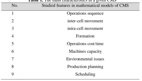
Table 1. The main characteristics in a given CMS No. Studied features in mathematical models of CMS

1 Operations sequence

2 inter-cell movement

3 intra-cell movement

4 Formation

5 Operations cost/time

6 Machines capacity

7 Environmental issues

8 Production planning

9 Scheduling

In this regard, 20 papers are investigated in detail which could be representatives of many papers in CMS. This investigation is reported in Table 2 based on the following categories.

(3)

228

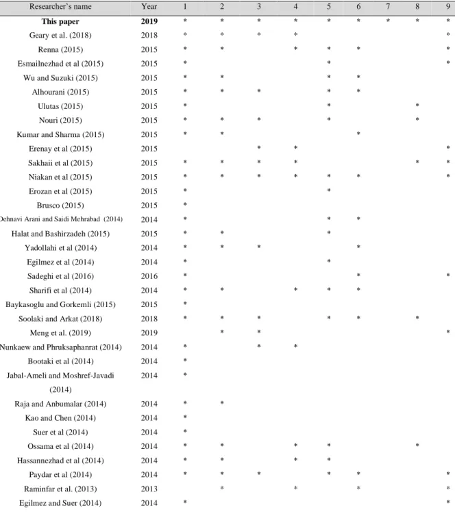
Table 2. The details of carried out researches in CMS

Researcher’s name Year 1 2 3 4 5 6 7 8 9

This paper 2019 * * * * * * * * *

Geary et al. (2018) 2018 * * * * *

Renna (2015) 2015 * * * * * *

Esmailnezhad et al (2015) 2015 * * *

Wu and Suzuki (2015) 2015 * * * *

Alhourani (2015) 2015 * * * * *

Ulutas (2015) 2015 * * *

Nouri (2015) 2015 * * * * *

Kumar and Sharma (2015) 2015 * * *

Erenay et al (2015) 2015 * * *

Sakhaii et al (2015) 2015 * * * * * *

Niakan et al (2015) 2015 * * * * * * *

Erozan et al (2015) 2015 * *

Brusco (2015) 2015 *

Dehnavi Arani and Saidi Mehrabad (2014) 2014 * * * Halat and Bashirzadeh (2015) 2015 * * *

Yadollahi et al (2014) 2014 * * * *

Egilmez et al (2014) 2014 * *

Sadeghi et al (2016) 2016 * * *

Sharifi et al (2014) 2014 * * * * * Baykasoglu and Gorkemli (2015) 2015 *

Soolaki and Arkat (2018) 2018 * * * * * *

Meng et al. (2019) 2019 * * *

Nunkaew and Phruksaphanrat (2014) 2014 * * * Bootaki et al (2014) 2014 *

Jabal-Ameli and Moshref-Javadi (2014)

2014 *

Raja and Anbumalar (2014) 2014 * * Kao and Chen (2014) 2014 *

Suer et al (2014) 2014 *

Ossama et al (2014) 2014 * * * * *

Hassannezhad et al (2014) 2014 * * * *

Paydar et al (2014) 2014 * * * * * *

Raminfar et al. (2013) 2013 * * * *

Egilmez and Suer (2014) 2014 * *

As it could be seen from table 2, few studies have investigated CMS quantitatively, while environmental issues in presence of machine- part scheduling have not been explored so far. In this paper, a mathematical model for designing the CMS is proposed in which mentioned features are taken into accounts such as environmental issues, part processing scheduling, dynamic modeling, wastes reduction, and production planning.

In section 2 the mathematical model including assumptions is stated. Subsequently, model linearization, as well as the robust model, is presented followed by the main model. Then, several sample instances are used to assess the proposed model. Finally, conclusions and future studies are presented.

2- Mathematical modeling

This model is designed for a multidirectional production system. The proposed model is a non-linear mixed integer model, which considers the configuration of cells and timing of operations along

(4)

229

production planning. At first, a nonlinear mathematical model is presented for the desired problem. The proposed model includes minimizing the cost of moving parts, fixed and variable costs of using machines, the cost of waste amount of machines (Wu et al. 2016), energy consumption costs of machinery, operator costs, and minimization of processing time. In fact, the model presented in this paper follows the three main objectives of creating proper cell layout, scheduling operations on different machines and being green issues.

Since the proposed model is complex in terms of solution, firstly the functions and constraints related to the creation of the layout are considered. After linearizing model using the relevant techniques, it will be solved by GAMS optimization software.

The output of this part of the model is considered as the input for the second part of the problem, i.e., the operation scheduling. To solve the scheduling problem, a meta-heuristic algorithm of ICA has been used and it is coded using MATLAB. Finally, in order to evaluate the quality of the solutions, 30 different problems were solved in small, medium and large scales. In this section, we present the main assumptions of the proposed model.

Assumptions:

 The number of parts in a production period is certain and predefined.  Processing of all parts should be performed in a period.

 Each part has a series of burst operations that must be done. But there is no priority between component processing.

 Each part of operation is machineries out at a workstation. All machines can process parts.  All operators can process parts.

 Processing time can vary with each machine and operator.  Each operation requires a machine and an operator.

 Operation cannot be stopped. So if the activity starts, it will continue until the end.  All parameters of the definitive model are assumed.

c1,2, .,C



t Index for manufacturing technology t1, 2, ,T

r

Index for time



r0,1,2, ,R



Input parameters:

-pkmwt

S

The processing time of the (k) operation of on the (m) machine and the operator (w) in the

(5)

230 mt



Overhead and maintenance of the (m) machine during the production period (t) mt



Machine (m) operating cost per unit time in production period (t) wt

F S

The fixed cost of using the operator (w) in the production period (t) wt

VS

The variable cost of using the operator (w) per unit time in the production period (t) pt



Intercellular cost of part (p) during production period (t) ut

B

The upper limit of cell capacity during the production period (t) dt

B

The lower limit of cell density during the production period (t)

pklt

R The parameter 0 and 1, if the (k) operation of the p-part can be made during the production

period (t) on the workstation (l), is 1 and otherwise 0.

mlt

O

The energy consumption of the machine (m) during the production period (t), which is installed

at the workstation (l).

pkmt

E The fractional cost of (p) in k operations during the production period (t) when processed by the

(m) machine.

pt

D Existing demand for (p) part in production period (t).

pt

r

 The cost of maintaining the (p) part in the production period (t).

pt

r

 _{The cost of shortage and removal of the (}_p_{) part in the production period (}_t_).

mt

r



Machine power consumption (m) at extra time during production (t). mt

Tr



Maximum time of machine (m) at normal time during production (t).

mt

Fr



Maximum time of the machine (m) in the extra time during the production period (t). Decision variables:

mlt

X

If the machine (m) is in the production period (t) at the workstation (l) is 1, otherwise it will be 0.

wlt

Y

If the operator (w) is in the production period (t) at the workstation (l), is 1, otherwise it will be 0.

clt

(6)

231

pklt

Q If the (k) operation of the part (p) is processed during the production period (t) at the work station

(l), then the value is 1, otherwise it will be 0.

pkrt

A If the (k) operation of the part (p) is processed during the production period (t) at time (r), it is 1,

otherwise it will be 0. (Time is considered discrete)

pt

QB _{If (}_p_{) is generated during production (}_t_{), it is 1, otherwise it will be 0.}

pkt

J The processing time of the (k) operation on (p) during the production period (t). h

wj

RQ Amount of part j should be produced in period h by supplier w.

pt

Ir _{The amount of excess product produced by part (}_p_{) during the production period (}_t).

pt

Br The demand for recovered part (p) during the production period (t)

pt

Qr The production rate of (p) during production (t).

mt

(7)

232

2-1- Non-linear mathematical formulation

In this section, a mixed-integer nonlinear mathematical programming model is presented based on the information presented below.

min Model1

(k 1) lt (k 1) lt

1 1 1 1 1 1

1

2

p

K

T P C L L

pklt pklt clt p p clt pt pt

t p k c l l

R

Q

Z

R

_

Q

_

Z



Qr

     























   



(1)

1,...P

1 1 1 1 1 0

( ) ( ) FS max ( J )

p p

T M L W L R

mlt mt wlt wt _p pK rt pK t

t m l w l r

X



Y tA



     

 

 _  _ 

 

  

 



(2)

1 1 1 1 1 1

(

VS )

T L P L M W

pklt pklt pt mlt wlt pkmwt mt wt

t l p l m w

R

Q

Qr X

Y

S



     







₍₃₎

1 1 1 1 1

p K

T M P L

pkmt mlt pklt t m p k l

E X Q

    





(4)

1 1 1 1 1

p K

T M P L

pkmt mlt pklt t m p k l

E X Q

    





(5)

1 1 T P pt pt t p

r Ir



 





₍₆₎

1 1 T P pt pt t p

r Br



 





₍₇₎

1 1

T M

mt mt

t m

time



r

 





₍₈₎

s.t. 1 1 , L mlt l

X m t



 



(9)

1

1 ,

L wlt l

Y w t



 



(10)

1

1 ,

M mlt m

X

l t









(11)

1

1 ,

W wlt w

Y l t



 



(12)

1

1 ,

C clt c

Z l t



 



(13)

1

1 , ,

L pklt l

Q

p k t



(18)

( 1) r

0 0

, ;

1, 2,...,

1

R R

p k t pkrt pkt p

r r

rA

_

rA

J

p t

k

K

 













(19) 0 1 max(0,t J )

1 , r, t

P

pk

K

P t

pkrt pklt pklt p k bn

A

R

Q

l

   





 

(20)

1 1 1

, ,

M L W

pkt pklt mlt wlt pkmwt

m l w

J

Q

X

Y

S

p k t

  







₍₂₁₎

1 1 1

,

p K _W _P

pt pklt mlt pkmwt mt mt k w p

Qr Q X S Tr time m t

  



  



(22)

( 1) ( 1) ,

pt pt p t pt pt p t

Qr D Ir _ Ir Br Br _ p t (23) ,

pt pt

Qr M QB_ p t (24)

,

mt mt

time



FR





m t

(25)

,

{0,1}

, , , , , ,

int .

, ,

,

0 , , ,

ml wl cl pkl pkrt pt

pkt

pt pt pt mt mt

X

Y

Z

Q

A

QB

m t l p k r c

J

t p k

Qr

Ir

Br Tr

time

m t p k















(26)

Objective function:

The objective function presented in the above model includes the minimization of 5 sentences, in which we will outline the concepts of each one. The term 1 is to minimize intercellular movement costs of parts. The term 2 is to minimize the fixed cost of using machines and operators, as well as minimizing the total processing time of parts. The phrase 3 is to minimize the variable cost of using machines and operators in the production system. The phrase 4 and phrase 5 are the criteria for the greenness of the model.

These two objective functions will minimize the amount of energy consumed in the system and the amount of waste generated by the machinery. The phrase 6 and clause 7 will minimize the costs of keeping and disposing parts during production periods. Finally, the phrase 8 relates to the amount of energy consumed by the machine during overtime, which is not desirable and should be minimized.

Constraints:

The concepts of constraints related to the above model are also discussed below. Constraint (9) states that each machine is to be located only in one workstation. Constraint (10) imposes the same restriction on the operator. Constraint (11) specifies the number of machines that can be located at a workstation, which can have a maximum of 1 machine per problem. The same limitation is applied to the operator using Constraint (12). Constraint (13) states that each workstation can be created in just one cell. Each operation must be done at a workstation for each part. This is

(9)

234

expressed by Constraint (14). This assignment can also be done if the desired work station is capable of processing the operation, which is satisfied by inequality. Constraints (16) and (17) determine the upper and lower limit of cell capacity to create work stations. The start time of each operation in this environment begins with constraint (18). As mentioned earlier, in this time model, discrete intervals are considered. Constraint (19) states that the time to start the next operation of a part should be as long as the duration of the previous operation, which is a limitation of a reasonable time limit. Constraint (20) is to adhere this, so that a maximum of one operation per workstation can be in progress at a given time. Constraint (21) shows the total processing time of an operation for each part, which is naturally calculated by considering the variables shown. Constraint (22) Indicates the machine's working capacity in typical times and over-runs. Constraint (23) determines the balance of inventory in a production system, which in fact is the amount of goods produced in a period equal to the amount of demand for that commodity at that time and the inventory and the amount of its disposal. Constraint (24) indicates the condition of performing or not processing a part in a production period. Constraint (25) indicates the maximum overtime capacity for the machine. Finally, constraint (26) indicates types of variables considered.

Linearizing the relevant model:

Since the model presented in this paper is a nonlinear model, it first converts to a linear model

. using linearization techniques

We first consider the model regardless of scheduling sentences and then perform the linearization operation as follows. In this regard, we use the techniques expressed in Bagheri and Bashiri's research (Bagheri and Bashiri, 2014).

Equation (1) The objective function and the relevant constraints will be linearized in this way :

1

1 1 1 1

1

( )

2

p K

T P C

pt

t p k c

E



   

 

  

(27)

klt (k 1) lt (k 1) lt 1

1 1

, , ,

L L

pklt cp p cp

l l

R QrQZ R _ QrQZ _ E p k t c

 

  



(28)

(k 1) lt (k 1) lt klt 1

1 1

, , ,

L L

p cp pklt cp

l l

R _ QrQZ _ R QrQZ E p k t c

 

  



(29)

(k 1) lt , ,

cp pt

QrQZ _ Qr p l c(30)

(k 1) lt , , , ,

cp pklt

QrQZ _ M Q_ p k t c l (31)

(k 1) lt , , , ,

cp clt

QrQZ _ M Z_ p k t c l (32)

(k 1) lt (2 ) , , , ,

cp pt clt pklt

QrQZ _ Qr  Z Q M_ p k t c l (33)

Equation (3) The objective function and the related constraints will be linearized in this way :

1 1 1 1 1 1

(

VS )

T L P L M W

pklt pkltmw pkmwt mt wt

t l p l m w

R

QQRXY

S



     





(34)

, , , , ,

pkltmw pt

QQRX Y Qr p k t m l w (35) , , , , ,

pkltmw pklt

QQRX Y M Q_ p k t m l w ₍₃₆₎

, , , , ,

pkltmw mlt

QQRX Y M X_ p k t m l w ₍₃₇₎

, , , , ,

pkltmw wlt

(10)

235

(3 ) , , , , ,

pkltmw pt pklt mlt wlt

QQRX Y Qr  Q X Y M_ p k t m l w (39)

3- Solution method

3-1- Imperialist Competitive Algorithm

After determining the location of machines and cells, in the second stage, using an Imperialist Competitive Algorithm (ICA) implemented on MATLAB software, the timing of the parts was machineries out. The ICA is an evolutionary new algorithm that can be categorized as a class of modern meta-innovations. The overall goal of the optimization algorithm is to simulate the competition of the world's top powers to obtain more pollutants.

This algorithm, like other evolutionary optimization methods, begins with a number of random primitive populations in the Genetic Algorithm (GA). Some of the best elements of the population are chosen as the imperialist or colonial equivalent of the elites in GA. And the rest of the population is considered as colonies.

Every member of the population is called a nation. Countries are divided into colonies and colonizers. The criterion for distinguishing between these two categories is the power of each country. In other words, powerful countries have ownership of poor countries. The power criterion can be the same objective function in the desired issues. So, you can use the term cost instead of the word power in most of the minimization issues.

(

)

n

c



f country

The normalized cost of each country in each state is obtained using the following equation:

max ( )

n n i

C



c



c

In order to better compare the colonial countries, the costs associated with these countries can be normalized using the following equation :

_

1

i i n imp

i i

C p

C





In the above relation n_imp shows the number of imperialists.

The total cost of a state can be obtained using the following equation:

_ _ cos _i _ cos _i max( _ cos )

normal Total t Total t  Total t

In the next step, the probability of capturing a country-usually the weakest colony of a weak state-will be calculated by an imperialist :

_

1

_ _ cos

_

_ _ cos

i i n imp

i i

normal Total t p total

normal Total t





In fact, we can say that this algorithm consists of two basic parts. The first section is absorption policy, which is an in-state phenomenon and the second part of the imperial competition, an interstate phenomenon.

Colonial countries, depending on their power and the policy of absorbing (aligning) along with various optimization axes, push the colonial countries to their own side.

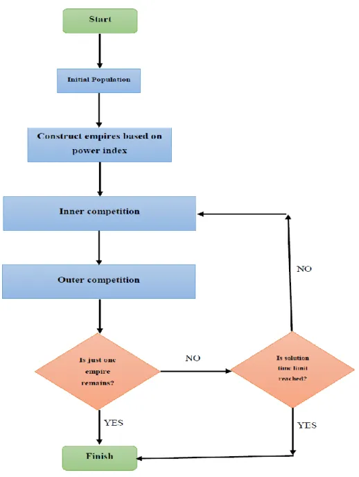
In other words, within each state, the colonies always try to progress from different aspects of political, economic, military, and so on. But to do this, they need a pattern to move in, and the best pattern can be the strongest power in the region. And this is what happens in this algorithm. The overview of the algorithm is shown in the figure below.

(11)

236

Fig 1. The Appearance of Imperialist Competitive Algorithms

If during a move a colony finds a better position than the colonizer, the two will change together. The mode of movement is such that each answer (the country) approaches x and the theta angle to the top imperial answer, x is a random number with a uniform distribution or any other uniform distribution.

In general, 𝑥 ≈ 𝑈(0, 𝛽 × 𝑑) is a number larger than one, and because of this, the imperialist movement is used in all directions. It is shown that





2

value is a suitable fit for finding acceptable solutions.

The existence of a theta will increase the space of the answer. So that all countries do not approach the imperialist just in a single direction. Theta can be considered as 𝜃 ≈ 𝑈(−𝛾, 𝛾). With the formation of primitive empires, imperialist competition begins between them. The survival of an empire to its power is to capture the colonies of competing empires and to dominate them.

During the colonial rivalry, weak empires gradually lose their power and disappear over time, and with the continuation of this process, we find that there is only one emperor in the world (reaching the optimal point).

Therefore, the survival of an empire will depend on its power to capture the colonies of rival empires, and to dominate them. Over time, the colonies will be closer to the empire in power, and we will see a kind of convergence. The ultimate colonial rivalry is when we have a single empire in the world, very close to the imperialist countries with the status quo.

After intra-state moves and the stabilization of countries, competition between imperialists begins. First, the weakest state (higher cost) is selected, and the weakest country in the state will emerge from the capture of that imperialist. It will be captured by these countries, given the possibility of further capture by the imperialists. This can be done with the following algorithm:

A: Create the vector p of the probabilities of seizing each imperialist:



_

1

, _

2

,..., _

n imp_



P



p total p total

p total

B: Create an R vector as follows:

𝑅 = {𝑟1, 𝑟2, … , 𝑟𝑛_𝑖𝑚𝑝} 𝑟 ≈ 𝑈(0,1)

C: Make D vector:



1

,

2

,...

n imp_



D

  

P

R

d d

d

D: The imperialist who receives the highest value of D in its index would capture the new country. This process will go on until only one state remains with an imperialist whose answer is optimal (or near optimal).

The effective parameters of the initial population algorithm are the number of imperialists,

, and .

 



:



As mentioned, this value should be greater than 1 in order to move from one side to the imperial.

(12)

237 :



Determines the degree of deviation from the course of the colonial movement towards the imperialist.

:



Indicates the importance of each colony in determining the overall state of the state.

Each of the above values should be machine fully determined. The reason for this is that the speed of convergence and the resolution of the problem (in NP-Hard) strongly depends on these parameters. Therefore, any inaccuracy in determining the correctness of these factors will slow down the algorithm or maybe incorrect answers.

3-2-Implementation of imperialist competitive algorithm

In this paper, this algorithm is developed for a discrete problem. How to display the answer in a discrete way and move the answers towards the colonizer using combinatory and mutation operators (defined in the GA).

The flowchart used in this article is based on this method:

Fig 2. Semi- Imperialist Competitive Algorithm

(13)

238

be solved using the ICA in MATLAB software. The purpose of this is to determine the order of the processing of parts and their assignment to machinery that can process the parts. In fact, the main variables expressed in the proposed model, which are related to the timing of the activity, are the time to start processing the components and allocate them to the machines, which are considered in terms of how the answer is presented, as described below.

3-3- Solution representation

In the colonial competition algorithm used in this paper, each answer is shown as follows:

In this coding, each answer is represented by a two-part response string. The first part indicates the order of the different parts, and the second part represents the machine in which each of the parts will be processed on that machine. For example, in the following thread, the parts 2, 3, 1, and 4 will be processed on machines 1, 3, 2, and 1, respectively. The last number in this thread indicates the goal function, which is the earliest completion time of the activity with this answer.

Fig 3. Representation of the solution

In the interstate competition stage, solutions should be combined to improve. The strategy used in this section includes 2 items:

A: Changes in the order of processing the part:

In this section, changes to the first part of the thread will be performed. For example, in the following figure, the order of operations, which is 2, 3, 1, and 4, is reversed. The result is worse and has reached 12.

Parent: 2 3 1 4 1 3 2 1 10

child: 4 1 3 2 1 2 3 1 12

Fig 4. The answer B: Change in the allocation of the part to the machine:

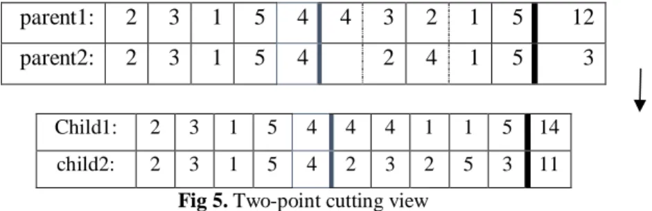
In this section, changes are made to the second part of the thread. For example, in the following figure, the combination of two-point cutting is used to generate a new answer, and two new solutions are derived from the combination of two solutions. As we can see, a better quality answer is created in this combination.

2 3 1 4 1 3 2 1 10

parent1: 2 3 1 5 4 4 3 2 1 5 12 parent2: 2 3 1 5 4 2 4 1 5 3

Child1: 2 3 1 5 4 4 4 1 1 5 14 child2: 2 3 1 5 4 2 3 2 5 3 11

Fig 5. Two-point cutting view The pseudo code used for this algorithm is as follows:

1- Input the initial parameters such the number of iterations as

n

_iand

populationsize

. 2-

1,

t



1

apply the second crossover on machine assignment.

9- For the last member of group apply the first crossover on operation sequence on the second one on machine assignment.

10-Correct the infeasible solutions and calculate the objective function. 11-If

n



n

_i finish, else go to 5.

4- Numerical computations

4-1-The CPLEX algorithm (phase1)

The model presented in this article is a complex model for solving capabilities. Therefore, an appropriate solution approach should be considered for medium and large dimensions. This paper uses a hierarchical approach to solving the proposed model.

First, the proposed model is solved without considering the scheduling sentences using the CPLEX algorithm and with the GAMS software. In order to evaluate the performance of the model presented in this section, several numerical examples have been developed and examined. The results are as follows (table 3 and table 4):

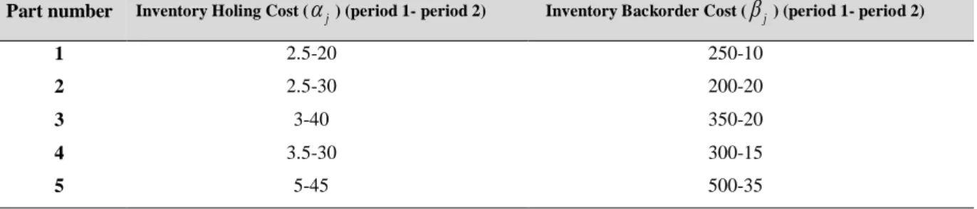
Table 3. Parts inventory information.

Inventory Backorder Cost (_j) (period 1- period 2) Inventory Holing Cost (_j) (period 1- period 2)

Part number

250-10 2.5-20

1

200-20 2.5-30

2

350-20 3-40

3

300-15 3.5-30

4

500-35 5-45

5

Table 4. Machinery information

) period 2 -period 1 ) (



h i

( Machine Extra Time Cost Machine number

1-0.5

1

1.5-1

2

0.9-2

3

0.8-0.5

4

0.9-0.5

5

According to table 5, for example, in the first production period, cell No.1 is located at candidate number 2 where machines 1 and 5 are located in that cell, and the second production period of the second place of cell 1 remains unchanged and only the machine The vehicles in which they were stationed changed into machines 2, 3 and 5.

(15)

240

Table 5. Intercellular layout and cell configuration response

Period 1 Period 2

Cells Locations Machines Locations Machines

1 2 5,1 2 5,3,2

2 3 2,3,4 3 1,4

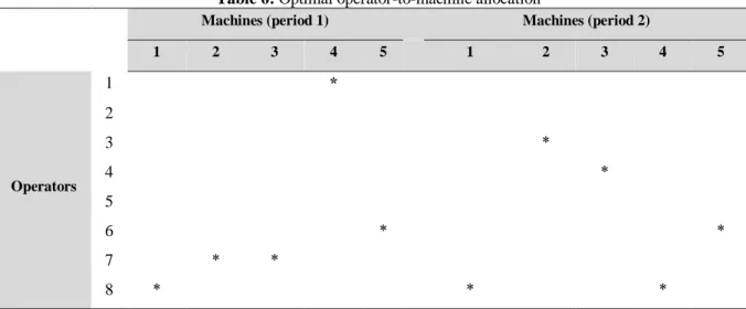
According to table 6, which deals with the optimal allocation of operators to any machine in each period, it can be noted that only operators 6 and 8 are assigned to similar machines in each production period and Other allocations have changed from the first period to the second period.

Table 6: Optimal operator-to-machine allocation

Machines (period 1) Machines (period 2)

1 2 3 4 5 1 2 3 4 5

Operators

1 *

2

3 *

4 *

5

6 * *

7 * *

8 * * *

In this article, four numerical examples are used to evaluate the quality of the proposed model. It is worth noting that since the model presented in this article is nonlinear, after modeling the model, the GAM software is used to solve the model. The data of these four examples in Table 7 and their results are presented in table 8.

Table 7: Information on generated examples

Operators Cells

Periods Parts

Machines Instances

5 2

2 4

4 1

5 2

2 5

4 2

8 2

2 5

5 3

10 3

2 8

7 4

Table 8: Comparison of Linear and Nonlinear Models.

Solution time (Linear Model) Optimal solution

(Linear Model) Solution time

(Non Linear Model) Optimal solution

(Non Linear Model) Instances

46 182390

94 248300

1

10 181804

300 NA*

2

220 28011

420 28011

3

550 17366

600 NA

4

(16)

241

For example according to table 8, the optimal cost amount for NO.3 is 28011, which includes optimal cell location, how to configure the cells and how to assign the operator to the machine.

4-2- Imperialist competitive Algorithm (phase2)

Table 9 shows the data of the studied issues and the numerical results obtained. The preliminary information of these issues is derived from an article provided by Kacem, and Saad (Kacem et al. 2002) and (Saad et al. 2002). As outlined in this table, the algorithm presented in this paper has the ability to improve the quality of the solution obtained from previous studies (Wu et al. 2016).

Table 8. Solution of scheduling problems using the method presented in this article

Improvement % Objective Function

(Kacem & Hammadi.) Objective Function (ICA) Proposed by machines parts Instance

number Saad et

al. Kacem & Hammadi. 31 16 11 * 5 4 1 25 16 12 * 8 8 2 27 15 11 * * 7 10 3 - 7 7 * * 10 10 4

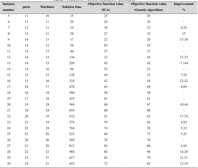
In table 8, examples 5 to 30 are generated randomly and display the good performance of the algorithm in a high dimension. In order to better evaluate the performance of the proposed algorithm, a genetic algorithm is used to compare the obtained results. As is clear from this table, most of the solutions obtained by the colonial competition algorithm were better than the genetic method.

Table 9. Random Number Indicators Generated

Improvement % Objective function value

(Genetic algorithm) Objective function value

(ICA) Solution time Machines parts Instance number - 25 25 15 10 11 5 - 29 29 20 11 11 6 6.25 32 30 34 11 12 7 15 32 27 28 11 13 8 15.38 26 22 17 11 14 9 - 63 63 58 12 14 10 - 27 27 46 13 14 11 33.33 45 32 136 14 14 12 -7.144 42 45 256 15 14 13 - 52 52 98 16 14 14 7.54 53 49 128 15 15 15 22.22 54 42 324 16 15 16 8.69 69 63 478 17 16 17 - 58 58 586 18 16 18 - 61 61 425 18 17 19 10.44 67 60 364 18 19 20 - 68 68 654 18 20 21 17.74 62 51 532 19 20 22 4.83 62 59 578 19 21 23 5.12 78 74 784 19 22 24 5.47 73 69 523 20 23 25 - 78 78 569 20 20 26 4.65 86 82 812 20 21 27 14.28 98 84 985 21 22 28 21.51 79 62 617 21 23 29 12.19 82 72 652 21 24 30

(17)

242

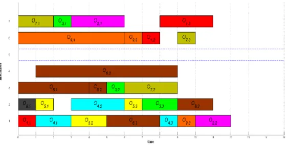
In the following, we will discuss schematically issue number two. The following figure shows an overview of the solution to problem 1. In this case, there are 8 parts and 8 machines, each operation of which will be processed on one of the existing machines. For example in this figure, yellow bars are related to operators of part 5. As it is clear from this figure, the operation will be completed at the time of the 12 scheduled times. In this figure, for example, part 5, which is marked with yellow, has three different operations, which will be processed on machines 2, 1 and 2, respectively.

Fig 6. Graphical view of instance 1

4-3- Sensitivity analysis

In this section, we analyze the sensitivity of the important parameters of the model, and evaluate the performance of the proposed method.

4-3-1- Sensitivity analysis of green parameters

In order to investigate the effect of environmental impacts and energy consumption, the two parameters considered for these two subjects have been modified in example 2 and the sensitivity of the objective functions toward them has been investigated. The graph below shows the results. As it is known, the increase in the cost of consuming energy in over-the-counter time will have a greater impact on the target functions and therefore this cost should be considered as an essential element. We only considered the environmental related costs in this figure in order to study the importance of different kinds of energy related effects.

Fig 7. Effects of environmental effects on the target function

0 50000 100000 150000 200000 250000 300000

2 0 4 0 6 0 8 0 1 0 0

O

B

JE

C

TI

V

E

FU

N

C

TI

O

N

V

ALU

E

INCRESING RATE (PERCENTAGE)

wast cost Energy cost in usual time

(18)

243 4-3-2- Sensitivity analysis of proposed model

The figure below shows the effect of doubling the processing time of different parts on the amount of target function. As you can see from this figure, the processing time of sections 2 and 6 has the greatest effect on the target function and its value is set to 15. Therefore, it is necessary to consider these components as critical components and to adopt appropriate management behavior regarding them.

In order to evaluate the performance of the proposed method more precisely, the processing time of the operation has been changed and its impact on the objective function has been investigated. In this case, Case Study No. 2 has been analyzed.

The figure below shows the effect of doubling the processing time of different parts on the amount of target function. As you can see from this figure, the processing time of Sections 2 and 6 has the greatest effect on the target function and its value is set to 15. Therefore, it is necessary to consider these components as critical components and to adopt appropriate management behavior regarding them.

In order to evaluate the performance of the proposed method more precisely, the processing time of the operation has been changed and its impact on the objective function has been investigated. In this case, Case Study No. 2 has been analyzed.

The figure below shows the effect of doubling the processing time of different parts on the amount of the objective function. As it can be seen, the processing time of parts 2 and 6 has the greatest effect on the objective function and its value is set to 15. Therefore, it is necessary to consider these components as critical components and to adopt appropriate management behavior regarding them.

Fig 8. The effect of doubling the processing time of components on the amount of target function

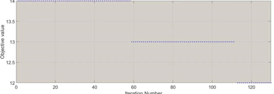
Figure 9 shows the objective value increasing trend versus the iteration numbers. As it is clear from this figure, the algorithm is converged to the optimal solution in 112th_iteration.

Fig 9. The objective value increasing trend versus the iteration numbers

12 12.5 13 13.5 14 14.5 15 15.5

1 2 3 4 5 6 7 8 9

T

im

e

(

Obje

ct

ive

fu

n

ct

ion

)

(19)

244

5- Conclusion and managerial insights

In this paper, a mathematical model for the design of a cell production system is presented with consideration of production planning. Consideration of environmental factors such as energy consumption and waste generated by machines in the proposed model are considered. Also, the problem of scheduling component processing in the presented model has been considered. Due to the complexity of the model presented in this paper, a hierarchical approach is proposed for solving the model. At first, the proposed model is analyzed without considering the scheduling topic using the GAMS software and the results are analyzed. Then a colonial competition algorithm was used to solve the scheduling problem.

To evaluate the performance of the proposed model, numerical examples are used in small, medium and large dimensions. Also, the colonial competition algorithm presented in this paper is compared with the methods available in the literature as well as the genetic algorithm and its quality is confirmed. Also, the parametric analysis machineries out in this paper provide several managerial approaches to the manager of production collections. The effect of increasing the amount of energy consumed during overtime is greater than the other environmental factors considered in this article, and therefore this cost should be controlled.

According to the model and the results, we introduce some managerial implications for more considerations as follows:

 According to the results, manufacturing systems with fewer cells were more efficient than larger formations. For systems that contain sequential production process, there was a loss in efficiency because of a differential in cell balance. The smaller sequential cells were more efficient than the larger serial cells, in part because the larger cells involve a longer serial chain, which constrains productivity to a degree.

 In order to increase efficiency of the scheduling aspects of the system, it is required to decrease the total inter-cell movements. By this way, the transportation time of parts between cells is dedicated from the total flow time and this can minimize completion time. To achieve such goal, the system tries to form minimum number of manufacturing cells.

 For improving the performance of greenness of the model, the managers should try to minimize the total consumed machine power in each period. For this purpose, the extra time of using machines should be replaced with production time of suppliers. Therefore, developing a network of suppliers will help the managers to improve the level of greenness of the manufacturing cells.

 Between-Cell Heterogeneity (BH) indicated a significant effect on system performance, consistently with the highest level of between-cell heterogeneity resulting in the highest system efficiency. This was consistent in almost all configurations. These results highlight the impact of the consideration of between-cell heterogeneity as part of workforce planning models. We note that not considering the heterogeneity between cells as part of the worker-cell assignment, could affect the accuracy of production estimates, and subsequently system performance.

Providing solutions for solving models with less time can be proposed as a future proposition. Also, considering the theory of queue as a factor affecting the quality of the scheduling provided, it will also be valuable in the presented framework

Disclosure statement

(20)

245

References

Alhourani, F. (2016). Cellular manufacturing system design considering machines reliability and parts

alternative process routings. International Journal of Production Research, 54(3), 846-863.

Bagheri, M., & Bashiri, M. (2014). A new mathematical model towards the integration of cell

formation with operator assignment and inter-cell layout problems in a dynamic environment. Applied

Mathematical Modelling, 38(4), 1237-1254.

Baykasoglu, A., & Gorkemli, L. (2015). Agent-based dynamic part family formation for cellular

manufacturing applications. International Journal of Production Research, 53(3), 774-792.

Bootaki, B., Mahdavi, I., & Paydar, M. M. (2014). A hybrid GA-AUGMECON method to solve a

cubic cell formation problem considering different worker skills. Computers & Industrial

Engineering, 75, 31-40.

Brusco, M. J. (2015). An iterated local search heuristic for cell formation. Computers & Industrial

Engineering, 90, 292-304.

Chang, C. C., Wu, T. H., & Wu, C. W. (2013). An efficient approach to determine cell formation, cell

layout and intracellular machine sequence in cellular manufacturing systems. Computers & Industrial

Engineering, 66(2), 438-450.

Deep, K., & Singh, P. K. (2015). Design of robust cellular manufacturing system for dynamic part

population considering multiple processing routes using genetic algorithm. Journal of Manufacturing

Systems, 35, 155-163.

Dehnavi-Arani, S., & Mehrabad, M. S. (2014). A two-stage model for cell formation problem

considering the inter-cellular movements by automated guided vehicles. Journal of Industrial and

Systems Engineering, 7(1), 43-55.

Egilmez, G., & Süer, G. (2014). The impact of risk on the integrated cellular design and

control. International Journal of Production Research, 52(5), 1455-1478.

Egilmez, G., Erenay, B., & Süer, G. A. (2014). Stochastic skill-based manpower allocation in a

cellular manufacturing system. Journal of Manufacturing Systems, 33(4), 578-588.

Erenay, B., Suer, G. A., Huang, J., & Maddisetty, S. (2015). Comparison of layered cellular

manufacturing system design approaches. Computers & Industrial Engineering, 85, 346-358.

Erozan, I., Torkul, O., & Ustun, O. (2015). Proposal of a nonlinear multi-objective genetic algorithm

using conic scalarization to the design of cellular manufacturing systems. Flexible Services and

Manufacturing Journal, 27(1), 30-57.

Esmailnezhad, B., Fattahi, P., & Kheirkhah, A. S. (2015). A stochastic model for the cell formation

problem considering machine reliability. Journal of Industrial Engineering International, 11(3),

375-389.

Geary, J., Hubbard, E., King, B., Hahn, D., Clark, K., & Sturtevant, O. J. (2018). Automated resource

based scheduling system for cellular product manufacturing. Cytotherapy, 20(5), S74-S75.

Halat, K., & Bashirzadeh, R. (2015). Concurrent scheduling of manufacturing cells considering

sequence-dependent family setup times and intercellular transportation times. The International

(21)

246

Hassannezhad, M., Cantamessa, M., Montagna, F., & Mehmood, F. (2014). Sensitivity analysis of

dynamic cell formation problem through meta-heuristic. Procedia Technology, 12, 186-195.

Jabal-Ameli, M. S., & Moshref-Javadi, M. (2014). Concurrent cell formation and layout design using

scatter search. The International Journal of Advanced Manufacturing Technology, 71(1-4), 1-22.

Jolai, F., Tavakkoli-Moghaddam, R., Golmohammadi, A., & Javadi, B. (2012). An

Electromagnetism-like algorithm for cell formation and layout problem. Expert Systems with Applications, 39(2),

2172-2182.

Kacem, I., Hammadi, S., & Borne, P. (2002). Approach by localization and multiobjective

evolutionary optimization for flexible job-shop scheduling problems. IEEE Transactions on Systems,

Man, and Cybernetics, Part C (Applications and Reviews), 32(1), 1-13.

Kao, Y., & Chen, C. C. (2014). Automatic clustering for generalised cell formation using a hybrid

particle swarm optimisation. International Journal of Production Research, 52(12), 3466-3484.

Krishnan, K. K., Mirzaei, S., Venkatasamy, V., & Pillai, V. M. (2012). A comprehensive approach to

facility layout design and cell formation. The International Journal of Advanced Manufacturing

Technology, 59(5-8), 737-753.

Kumar, S., & Sharma, R. K. (2015). Development of a cell formation heuristic by considering

realistic data using principal component analysis and Taguchi’s method. Journal of Industrial

Engineering International, 11(1), 87-100.

Mahdavi, I., Teymourian, E., Baher, N. T., & Kayvanfar, V. (2013). An integrated model for solving

cell formation and cell layout problem simultaneously considering new situations. Journal of

Manufacturing Systems, 32(4), 655-663.

Meng, L., Zhang, C., Shao, X., & Ren, Y. (2019). MILP models for energy-aware flexible job shop

scheduling problem. Journal of cleaner production, 210, 710-723.

Niakan, F., Baboli, A., Moyaux, T., & Botta-Genoulaz, V. (2016). A new multi-objective mathematical model for dynamic cell formation under demand and cost uncertainty considering social

criteria. Applied Mathematical Modelling, 40(4), 2674-2691.

Nouri, H. (2016). Development of a comprehensive model and BFO algorithm for a dynamic cellular

manufacturing system. Applied Mathematical Modelling, 40(2), 1514-1531.

Nunkaew, W., & Phruksaphanrat, B. (2014). Lexicographic fuzzy multi-objective model for

minimisation of exceptional and void elements in manufacturing cell formation. International Journal

of Production Research, 52(5), 1419-1442.

Ossama, M., Youssef, A. M., & Shalaby, M. A. (2014). A multi-period cell formation model for

reconfigurable manufacturing systems. Procedia CIRP, 17, 130-135.

Paydar, M. M., Saidi-Mehrabad, M., & Teimoury, E. (2014). A robust optimisation model for

generalised cell formation problem considering machine layout and supplier selection. International

Journal of Computer Integrated Manufacturing, 27(8), 772-786.

Rafiei, H., & Ghodsi, R. (2013). A bi-objective mathematical model toward dynamic cell formation

(22)

247

Raja, S., & Anbumalar, V. (2016). An effective methodology for cell formation and intra-cell machine layout design in cellular manufacturing system using parts visit data and operation sequence

data. Journal of the Brazilian Society of Mechanical Sciences and Engineering, 38(3), 869-882.

Raminfar, R., Zulkifli, N., Vasili, M., & Sai Hong, T. (2013). An integrated model for production

planning and cell formation in cellular manufacturing systems. Journal of Applied Mathematics, 2013.

Renna, P., & Ambrico, M. (2015). Design and reconfiguration models for dynamic cellular

manufacturing to handle market changes. International Journal of Computer Integrated

Manufacturing, 28(2), 170-186.

Saad, S. M., Baykasoglu, A., & Gindy, N. N. (2002). A new integrated system for loading and

International Journal of Computer Integrated

scheduling in cellular manufacturing. .

49 -37 ), 1 (

15

,

Manufacturing

Sadeghi, S., Seidi, M., & Shahbazi, E. (2016). Impact of queuing theory and alternative process

routings on machine busy time in a dynamic cellular manufacturing system. Journal of Industrial and

Systems Engineering, 9(2), 54-66.

Sakhaii, M., Tavakkoli-Moghaddam, R., Bagheri, M., & Vatani, B. (2016). A robust optimization approach for an integrated dynamic cellular manufacturing system and production planning with

unreliable machines. Applied Mathematical Modelling, 40(1), 169-191.

Satoglu, S. I., & Suresh, N. C. (2009). A goal-programming approach for design of hybrid cellular

manufacturing systems in dual resource constrained environments. Computers & industrial

engineering, 56(2), 560-575.

Sharifi, S., Chauhan, S. S., & Bhuiyan, N. (2014). A dynamic programming approach to GA-based

heuristic for multi-period CF problems. Journal of Manufacturing Systems, 33(3), 366-375.

Soolaki, M., & Arkat, J. (2018). Supply chain design considering cellular structure and alternative

processing routings. Journal of Industrial and Systems Engineering, 11(1), 97-112.

Süer, G. A., Ates, O. K., & Mese, E. M. (2014). Cell loading and family scheduling for jobs with

individual due dates to minimise maximum tardiness. International Journal of Production

Research, 52(19), 5656-5674.

Tavakkoli-Moghaddam, R., Javadian, N., Khorrami, A., & Gholipour-Kanani, Y. (2010). Design of a scatter search method for a novel multi-criteria group scheduling problem in a cellular manufacturing

system. Expert Systems with Applications, 37(3), 2661-2669.

Ulutas, B. (2015). Assessing the number of cells for a cell formation problem.

IFAC-PapersOnLine, 48(3), 1122-1127.

Wu, B., Fan, S., Yu, A. J., & Xi, L. (2016). Configuration and operation architecture for dynamic

cellular manufacturing product–service system. Journal of cleaner production, 131, 716-727.

Wu, L., & Suzuki, S. (2015). Cell formation design with improved similarity coefficient method and

decomposed mathematical model. The International Journal of Advanced Manufacturing

Technology, 79(5-8), 1335-1352.

Wu, T. H., Chung, S. H., & Chang, C. C. (2010). A water flow-like algorithm for manufacturing cell

(23)

248

Wu, X., Chu, C. H., Wang, Y., & Yan, W. (2007). A genetic algorithm for cellular manufacturing

design and layout. European journal of operational research, 181(1), 156-167.

objective

-Yadollahi, M. S., Mahdavi, I., Paydar, M. M., & Jouzdani, J. (2014). Design a bi

cellular manufacturing systems considering variable failure rate of mathematical model for

. 7415 -7401 ), 24 (

52

,

International Journal of Production Research