Profile and wavefront optimization by metaheuristic algorithms for efficient finite element analysis

(1)

Sharif University of Technology

Scientia Iranica

Transactions A: Civil Engineering http://scientiairanica.sharif.edu

Invited Paper

Prole and wavefront optimization by metaheuristic

algorithms for ecient nite element analysis

A. Kaveh

a;

_{and Sh. Bijari}

b

a. Centre of Excellence for Fundamental Studies in Structural Engineering, Iran University of Science and Technology, Narmak, Tehran, P.O. Box 16846-13114, Iran.

b. School of Civil Engineering, Iran University of Science and Technology, Narmak, Tehran, P.O. Box 16846-13114, Iran. Received 25 December 2016; received in revised form 2 October 2017; accepted 28 January 2018

KEYWORDS Prole and wavefront reduction;

Ordering; Colliding Bodies Optimization (CBO); Enhanced Colliding Bodies Optimization (ECBO);

Tug of War

Optimization (TWO); Vibrating Particles System (VPS).

Abstract. To eciently solve the equations that arise from nite element analysis, the stiness matrix of a model should be structured. This can be achieved by reducing the prole or wavefront of the corresponding graph matrix of a structure depending on whether the skyline or frontal method is used. One of the ecient methods for achieving this goal is the method of King, extended by Sloan. In this paper, the coecients of the priority function utilized in the generalized Sloan's method are optimized using the recently developed metaheuristic algorithm, called vibrating particles system. The results are compared with those of other metaheuristic algorithms consisting of the particle swarm optimization, colliding bodies optimization, enhanced colliding bodies optimization, and tug of war optimization. These metaheuristics are used for optimum nodal numbering of the graph models of the nite element meshes to reduce the prole and wavefront of the corresponding sparse matrices. The comparison of the results of the metaheuristic algorithms and those of the King and Sloan demonstrates the eciency of the new metaheuristic algorithm utilized for prole and wavefront optimization.

1. Introduction

The solution to the sparse systems of simultaneous equations comprises every main element of many prob-lems in structural engineering. Such linear algebraic equations appear in the form of Ax = b arising from matrix structural analysis and nite element methods. These types of equations often involve a positive de-nite, symmetric, and sparse matrix coecient A. For large structures, a great deal of computational time and memory is usually dedicated to nding a solution *. Corresponding author. Tel.: +98 21 44202710;

Fax: +98 21 77240398

E-mail address: [email protected] (A. Kaveh) doi: 10.24200/sci.2018.20163

to these equations. Therefore, some suitable specic patterns for the coecients of the corresponding equa-tions have been provided such as banded form, prole form, and blocked form. These patterns can often be obtained by the nodal ordering of the corresponding models.

In the Finite-Element Model (FEM) analysis, when the nodes have one degree of freedom, performing nodal ordering is equivalent to reordering the equa-tions. In a more general problem, for each node with m degree of freedom, there are m coupled equations produced for each node. In such cases, re-sequencing is usually performed on the nodal numbering of the graph models to reduce the bandwidth, prole or wavefront, because the size of these problems is m-fold smaller than that with m degree of freedom numbering. In this article, the mathematical model

(2)

of the FEM is considered as an element clique graph, and nodal ordering is carried out to reduce the prole and wavefront of the corresponding matrices [1-3].

For nodal numbering in the solution of sparse sys-tems, the following rule can be used: permuting rows and columns of a matrix by the proper renumbering of the nodes of the corresponding graph. Two important parameters in nodal ordering are prole and wavefront optimization. In fact, for sparse matrices, the size of the problem can be measured by the prole or wavefront of such matrices. These problems produced considerable interest in the past because of its practical relevance for a signicant range of global optimization applications. Since the problem of nodal numbering is NP-Complete [4], many approximate approaches and heuristics have been proposed, examples of which can be found in Gibbs et al. [5], Cuthill and McKee [6], Kaveh [1], Bernardes and Oliveira [7], King [8], Kaveh and Behzadi [9], Kaveh and Roosta [10], and Koohes-tani and Poli [11].

Recently generated optimization methods consist of metaheuristic algorithms that solve complex prob-lems. These techniques explore a feasible region based on both randomization and some specic rules through a group of search agents. The rules are usually inspired by the laws of natural phenomena [12].

As a recently developed type of metaheuristic approach, Colliding Bodies Optimization (CBO) was introduced and employed in structural problems by Kaveh and Mahdavi [13]. CBO is a multi-agent method and is inspired by a one-dimensional collision between two agents. Each object is considered as a body with a specic mass and a velocity. A collision occurs between a pair of bodies, and the new positions of the colliding bodies are updated based on the laws of collision. The enhanced colliding bodies optimization introduced by Kaveh and Ilchi Ghazaan [14] employs memory in order to save the best-so-far position to improve the performance of CBO without increasing the computer execution time. This algorithm also utilizes a mechanism to escape local optima. A multi-agent metaheuristic algorithm, called tug of war opti-mization, was introduced by Kaveh and Zolghadr [15]. This technique models each candidate solution as a team engaged in a series of tug of war competitions. The weight of the teams is determined based on the quality of the corresponding solutions, and the value of pulling force that a team can exert on the rope is assumed to be proportional to its weight. VPS is a population-based optimization algorithm, which is inspired by a free vibration of a single degree of freedom systems with viscous damping, as was introduced by Kaveh and Ilchi Ghazaan [16]. In this method, the solution candidates are considered as agents that grad-ually approach their equilibrium positions. In order to ensure a proper balance between exploration and

exploitation, equilibrium positions are attained from the current population and the best historical position. The rest of this paper is organized as follows: in Section 2, some denitions of graph theory, prole, and wavefront are presented. CBO, ECBO, TWO, and VPS algorithms are briey stated in Section 3. In order to show the performance of these methods in reducing the prole and wavefront of the stiness matrix, eight examples are presented in Section 4. The last section concludes the present study.

2. Problem denition

2.1. Denitions from the theory of graphs Let G(N; M) be a graph with a set of members M(jMj = m) and a set of nodes N(jNj = n) together with a relation of incidence. The degree of a node is the number of members, which are incidental to that node; 1-weighted degree of a node is dened as the sum of the degrees of its adjacent nodes. A spanning tree is a tree containing all the nodes of S. The Shortest Route Tree (SRTn0) rooted in a considered node (starting node),

n0, is a spanning tree where the distance between every

node njof S and n0is minimum and where the distance

between the two nodes is taken to be the number of members in the shortest path between these nodes. A contour Cn0

k contains all the nodes with equal distance

k from node n0. The number of contours of an SRTn0

is known as its depth, denoted by d(SRTn0), and the

highest number of nodes in a contour shows the width of SRTn0. A label As of G assigns a set of integers

f1; 2; 3; ; ng to the nodes of graph G. As(i) is the label or the integer assigned to node i, and each node has a dierent label [2].

The prole of an N N matrix related to graph G, for the assignment process by As(i), is dened as follows:

PAs= N

X

i=1

bi; (1)

where the row bandwidth, bi, for row i is dened as

the number of inclusive entries from the rst nonzero element in the row to the (i + 1)th entry for this assignment. The eciency of the given ordering for the prole solution scheme corresponds to the number of active equations during each step of the factorization process. Formally, row j is dened to be active during elimination of column i if j i, and there exists aik= 0

with k i. Hence, in the ith stage of the factorization, the number of active equations is the number of rows of prole that intersect in column i, where the already eliminated rows are ignored. Let fi denote the number

of equations that are active during the elimination of variable xi. It follows from the symmetric structures

(3)

of the matrix that: PAs=

N

X

i=1

fi= N

X

i=1

bi; (2)

where fiis the frontwidth or wavefront. Assuming that

N and the average value of fi are considerably large,

it can be shown that a complete prole or front fac-torization needs approximately O(NF2

rms) operations,

where Frms is the root-mean square frontwidth, which

is dened as follows: Frms=

" 1 N N X i=1 f2 i #0:5 : (3)

For the purpose of obtaining an optimal nodal ordering in the prole and frontwidth reduction problems, the set of integers f1; 2; 3; ; ng should be assigned to the nodes of G using a priority function, and the coecients of the priority functions are obtained using PSO, CBO, ECBO, TWO, and VPS algorithms.

2.2. An algorithm based on priority queue for prole and wavefront reduction

The nodal numbering in a priority queue is carried out through the assignment of status based on the numbering approach of King [8]. King's method was generalized by Sloan [17] by introducing a priority queue that controls the order to be followed in the numbering of the nodes. This algorithm comprises two phases:

Phase 1: Selecting a pair of pseudo-peripheral (pseudo-diameter) nodes;

Phase 2: Nodal numbering.

In Phase 1, a pair of nodes is selected as starting and ending nodes according to the following steps:

Step 1: Choose an arbitrary node s of minimum degree;

Step 2: Generate the shortest route tree SRTs =

fCs

1; C2s; ; Cdsg rooted in s. Let S be the list of the

nodes of Cs

d, which is stored in the order of increasing

degree;

Step 3: Decompose S into subsets Sj of cardinality

jSjj, j = 1; 2; ; , where is the maximum

degree of any node of S such that all nodes of Sj are

characterized by degree j. Generate an SRT from each node y of S for the rst 1 mj . If

d(SRTy) > d(SRTs), then set s = y and go to Step 2;

Step 4: Let e be the root of the longest SRT that has the smallest width. When the algorithm terminates, s and e are the end points of a pseudo-diameter.

Figure 1. Dierent statuses of nodes.

In Phase 2 the nodes of an element clique graph are reordered, and it is ensured that the position of a node in this reordering phase follows a priority rule according to the following steps:

Step 1: Find the status of all nodes. A node can be found in one status of the following cases, as shown in Figure 1. A node that has been assigned a new label is considered as post-active. Nodes that are adjacent to a post-active node, yet do not have a post-active status, are called active. Each node which is adjacent to an active node, but is not post-active or active, is said to be pre-active. The nodes which are not post-active, post-active, or pre-active are considered as inactive; Step 2: Prepare a list of the candidate nodes, consisting of active and pre-active nodes, for labeling in the next step;

Step 3: Calculate the priority number of all the candidate nodes. For node i, the number is obtained from the following relationship:

Pi= W1 i W2 Di; (4)

where W1 and W2 are integer weights (suggested

as W1 = 1 and W2 = 2 in the original Sloan's

algorithm), i is the distance between each node i

and the end node, and Di is the incremental degree

of node i, which is dened as follows:

Di= di ci+ ki; (5)

where di is the degree of node i, ci is the number of

active and post-active nodes adjacent to node i, and ki is zero if node i is active or post-active, and unity

otherwise;

Step 4: Select the node with the highest priority among the candidate nodes and label it;

Step 5: Repeat Steps 1-4 until all the nodes of the graph are labeled.

In Eq. (4) if W1 = 0 and W2 = 1, the node labeling

algorithm becomes identical to the one proposed by King [8].

(4)

2.3. The priority function with new integer weights

According to Eq. (4), a linear priority function of two graph parameters is employed in Sloan's algorithm, and the weights determine the rank of each parameter. Sloan has recommended the pair W1= 1 and W2 = 2

for the weights. However, some research results show that, for some problems, using other values leads to better results.

The priority was generalized by Kaveh and Rahimi Bondarabdy [18] to a linear function of vectors of graph parameters as follows:

Fi= L

X

i=1

Wi Gi; (6)

where Gi (i = 1; 2; ; L) are the normalized Ritz

vectors representing the graph parameters, Wi (i =

1; 2; ; L) are the weights of the Ritz vectors (Ritz coordinates), which are unknown. That is, one can utilize L characteristics of a graph to dene the priority function and nd the weights that can guide the algorithm to choose an optimal prole or wavefront.

L = 2 characteristics of the graph model are employed in Sloan's algorithm. Here, we nd the best sets of weights for the priority function with L = 2 and 5. These sets of integer weights are found by utilizing PSO, CBO, ECBO, TWO, and VPS algorithms.

The method of L = 2 is presented as the rst case. The vectors of graph properties are taken similar to those of Sloan's strategy. In the second case, the method of L = 5, which uses ve vectors Gi (i =

1; 2; ; 5), is presented as follows:

- G1: Degrees of the nodes;

- G2: The node distance from the end node;

- G3: The node distance from the starting node;

- G4: The 1-weighted degree;

- G5: The width of an SRT rooted in the starting

node.

Once the vectors of graph parameters are formed, their weights can be obtained using PSO, CBO, ECBO, TWO, and VPS algorithms.

3. The utilized metaheuristic algorithms Metaheuristic algorithms have been previously utilized to optimize the coecients of the generalized Sloan function. Genetic algorithm [19], ant colony [20], charged system search [21], CBO, ECBO, and tug of war [22] are some of these applications. In this paper, VPS is added to the 3 algorithms used in the latter reference, and a more extensive comparison is made.

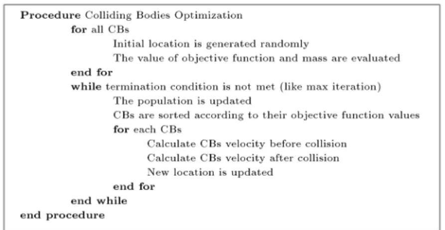
In this section, a brief description and pseudo codes of the colliding bodies optimization algorithm, its enhanced version, and then two new algorithms, called tug of War Optimization algorithm and vibrating particles system algorithm, are presented and employed to calculate the optimum values of the coecients. 3.1. Colliding bodies optimization

The collision between two objects is a natural phe-nomenon. The colliding bodies optimization technique was developed based on this occurrence by Kaveh and Mahdavi [13]. In this technique, one object collides with another and, thus, they move towards a minimum energy level. CBO utilizes a simple formulation, does not employ memory for saving the best-so-far solutions, and requires no internal parameter. For further details, reader mays refer to [13]. The pseudo code of CBO is provided in Figure 2.

3.2. Enhanced colliding bodies optimization Enhanced colliding bodies optimization is a modied version of CBO, which improves CBO to achieve highly reliable solutions, as was introduced by Kaveh and Ilchi Ghazaan [14]. The introduction of memory increases the convergence speed of ECBO more than that of CBO. Furthermore, changing some components of CBO helps ECBO escape local optima. For further

(5)

Figure 3. Pseudo code of the enhanced colliding bodies optimization algorithm.

Figure 4. Pseudo code of the tug of war optimization algorithm.

details, readers may refer to [14]. The pseudo code of ECBO is provided in Figure 3.

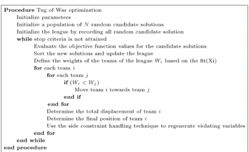
3.3. Tug of War Optimization (TWO) algorithm

TWO is a population-based metaheuristic algorithm, which was introduced by Kaveh and Zolghadr [15]. This approach models each candidate solution Xi =

fxi;jg as a team engaged in a series of tug of war

competitions. The weight of the teams is determined based on the quality of the corresponding solutions, and the value of pulling force which a team can exert on the rope is assumed to be proportional to its weight. Naturally, the opposite team will have to maintain at least the same value of force in order to sustain its grip of the rope. The lighter team accelerates toward the heavier team, and this forms the convergence

operator of TWO method. The method improves the quality of the solutions iteratively by keeping a proper exploration/exploitation balance and employing the described convergence operator. The pseudo code of TWO is provided in Figure 4.

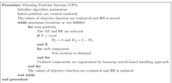
3.4. Vibrating particles system algorithm The vibrating particles system is a metaheuristic method and is inspired by the damped free vibration of single degree of freedom systems, as was introduced by Kaveh and Ilchi Ghazaan [16]. This approach involves a number of candidate solutions, representing the particles system. The particles are initialized randomly in an n-dimensional search space and grad-ually approach their equilibrium positions. To keep the balance between the exploration and exploitation, these equilibrium positions are achieved through the

(6)

Figure 5. Pseudo code of the vibrating particles system algorithm.

current population and the historically best position. The pseudo code of VPS is provided in Figure 5. 4. Numerical examples

In this section, eight Finite Element Meshes (FEMs) are considered. Element clique graph is a type of graph model that is employed for transferring topological properties of nite element models into connectivity properties of graphs [3]. The nodes of this graph model are the same as those of the corresponding nite element model with the nodes of each element being cliqued, and the multiple members in the entire graph are replaced by single members. Ten problems are presented to show the performance and eciency of some new optimization algorithms. Four test problems are presented by Everstine [23]. The well-known standard PSO algorithm, two new algorithms, namely the colliding bodies optimization and enhanced collid-ing bodies optimization, and two recently developed methods called tug of war optimization and vibrating particles system are applied to reduce the prole and wavefront. The results of the reduction of prole and wavefront with L = 2 and 5 methods are compared with those of the Sloan and King's algorithms in Tables 1 to 16, respectively.

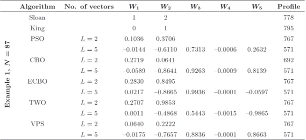
Example 1. A tower with 87 nodes and 227 elements is considered. The nite element mesh of this model is shown in Figure 6. The eciency of the above-mentioned algorithms is tested by this model for prole and wavefront reduction problems. The obtained results are given in Tables 1 and 2, respectively. The quality of the results is provided in these tables. Example 2. The schematic of a nite element model of power supply housing is presented in Figure 7. This

Figure 6. Schematic of the FEM of a tower.

Figure 7. Schematic of the FEM of power supply housing.

model has 307 nodes and 1108 elements. The results of prole and wavefront reduction problems by employing optimization algorithms are given in Tables 3 and 4, respectively.

(7)

Table 1. Comparison of the results of prole reduction for the tower problem.

Algorithm No. of vectors W1 W2 W3 W4 W5 Prole

Example

1,

N

=

87

Sloan 1 2 778

King 0 1 795

PSO L = 2 0.1036 0.3706 767

L = 5 {0.0144 {0.6110 0.7313 {0.0006 0.2632 571

CBO L = 2 0.2719 0.0641 692

L = 5 {0.0589 {0.8641 0.9263 {0.0009 0.8139 571

ECBO L = 2 0.2830 0.8495 767

L = 5 0.0217 {0.8665 0.9936 {0.0001 {0.0597 571

TWO L = 2 0.2707 0.9853 767

L = 5 0.0011 {0.4868 0.5443 {0.0015 {0.9865 571

VPS L = 2 0.0640 0.2222 767

L = 5 {0.0175 {0.7657 0.8836 {0.0001 0.8663 571 Table 2. Comparison of the results of wavefront reduction for the tower problem.

Algorithm No. of vectors W1 W2 W3 W4 W5 Frms

Example

1,

N

=

87

Sloan 1 2 8.7382

King 0 1 9.2189

PSO L = 2 0.2007 0.6255 9.6900

L = 5 0.0009 {0.5316 0.5742 {0.0009 0.5547 6.9124

CBO L = 2 0.2875 0.8730 9.6900

L = 5 0.0004 0.9800 {0.9047 {0.0008 0.3827 6.9124

ECBO L = 2 0.2428 0.8169 9.6900

L = 5 0.0005 {0.8408 0.9966 {0.0027 0.1399 6.9124

TWO L = 2 0.2727 0.9664 9.6900

L = 5 {0.1069 {0.6872 0.6581 {0.0040 0.8902 7.3085

VPS L = 2 0.0694 0.2674 9.6900

L = 5 0.0000 {0.7642 0.9004 {0.0022 0.0390 6.9124

Figure 8. Schematic of the hull w/renement model.

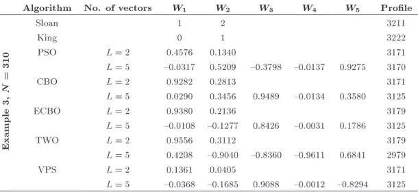
Example 3. A hull w/renement model containing 310 nodes and 1069 elements is considered in Figure 8. Tables 5 and 6 provide the values of the prole and wavefront reduction, respectively, and the results can be compared with those of these tables.

Figure 9. FEM of a barge.

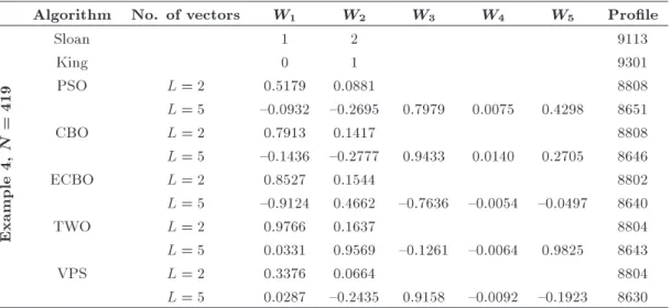
Example 4. The FEM of a barge with 419 nodes and 1579 elements is considered, as shown in Figure 9. Tables 7 and 8 provide the comparison results of prole and wavefront reduction problems by utilizing PSO, CBO, ECBO, TWO, and VPS algorithms for this example.

(8)

Table 3. Comparison of the results of prole reduction for the power supply housing problem.

Example

2,

N

=

307

Sloan 1 2 8730

King 0 1 9095

PSO L = 2 0.0042 0.2228 8205

L = 5 {0.0742 0.6049 {0.0674 0.0103 {0.5000 8421

CBO L = 2 0.0850 0.8204 8148

L = 5 0.0174 {0.2591 0.9308 {0.0035 0.1450 8262

ECBO L = 2 0.0546 0.9436 8205

L = 5 {0.0035 {0.0601 0.3642 {0.0010 {0.9357 8262

TWO L = 2 0.0248 0.3105 8189

L = 5 {0.5751 {0.8167 {0.1357 {0.5099 0.6424 8004

VPS L = 2 0.0168 0.2476 8205

L = 5 0.0009 {0.1628 0.9542 {0.0002 0.7594 8213 Table 4. Comparison of the results of wavefront reduction for the power supply housing problem.

Example

2,

N

=

307

Sloan 1 2 31.2292

King 0 1 32.0931

PSO L = 2 0.1578 0.9402 27.5724

L = 5 0.0105 0.1509 {0.9033 {0.0056 {0.6496 30.5202

CBO L = 2 0.1641 0.7762 30.6501

L = 5 {0.0375 {0.1102 0.9901 0.0056 {0.0212 28.426

ECBO L = 2 0.0777 0.9292 27.6011

L = 5 {0.0416 {0.0428 0.9934 0.0080 {0.0424 28.4111

TWO L = 2 0.0069 0.0459 27.2907

L = 5 {0.3605 {0.9187 {0.0700 {0.7603 {0.7260 27.2771

VPS L = 2 0.0368 0.7499 27.2907

L = 5 0.0042 {0.0490 0.8914 {0.0011 {0.3126 27.7194 Table 5. Comparison of the results of prole reduction for the hull w/renement model.

Example

3,

N

=

310

Sloan 1 2 3211

King 0 1 3222

PSO L = 2 0.4576 0.1340 3171

L = 5 {0.0317 0.5209 {0.3798 {0.0137 0.9275 3170

CBO L = 2 0.9282 0.2813 3171

L = 5 0.0290 0.3456 0.9489 {0.0134 0.3580 3125

ECBO L = 2 0.9380 0.2136 3179

L = 5 {0.0108 {0.1277 0.8426 {0.0031 0.1786 3125

TWO L = 2 0.9556 0.3112 3179

L = 5 0.4208 {0.9040 {0.8360 {0.9611 0.6841 2979

VPS L = 2 0.1361 0.0405 3171

(9)

Table 6. Comparison of the results of wavefront reduction for the rened nite element model.

Example

3,

N

=

310

Sloan 1 2 10.5232

King 0 1 10.5841

PSO L = 2 0.4899 0.1379 10.4361

L = 5 0.0326 {0.1466 0.7705 {0.0080 0.2158 10.2531

CBO L = 2 0.8400 0.2420 10.4108

L = 5 0.0115 {0.0681 0.4104 {0.0024 0.0422 10.2716

ECBO L = 2 0.8420 0.8420 10.4108

L = 5 {0.0502 {0.1924 0.8743 {0.0003 0.4107 10.2716

TWO L = 2 0.9624 0.2722 10.4108

L = 5 {0.7532 {0.6871 {0.6053 {0.9134 {0.0993 9.7714

VPS L = 2 0.5418 0.1575 10.4361

L = 5 {0.0307 {0.1404 0.8417 {0.0008 0.2558 10.2716 Table 7. Comparison of the results of prole reduction for the barge problem.

Example

4,

N

=

419

Sloan 1 2 9113

King 0 1 9301

PSO L = 2 0.5179 0.0881 8808

L = 5 {0.0932 {0.2695 0.7979 0.0075 0.4298 8651

CBO L = 2 0.7913 0.1417 8808

L = 5 {0.1436 {0.2777 0.9433 0.0140 0.2705 8646

ECBO L = 2 0.8527 0.1544 8802

L = 5 {0.9124 0.4662 {0.7636 {0.0054 {0.0497 8640

TWO L = 2 0.9766 0.1637 8804

L = 5 0.0331 0.9569 {0.1261 {0.0064 0.9825 8643

VPS L = 2 0.3376 0.0664 8804

L = 5 0.0287 {0.2435 0.9158 {0.0092 {0.1923 8630 Table 8. Comparison of the results of wavefront reduction for the barge problem.

Example

4,

N

=

419

Sloan 1 2 22.5524

King 0 1 23.0926

PSO L = 2 0.7145 0.1413 21.6733

L = 5 0.1294 0.7287 {0.2671 {0.0203 {0.2336 21.3466

CBO L = 2 0.9711 0.1722 21.6906

L = 5 {0.0756 0.8504 {0.2259 0.0063 {0.6770 21.2456

ECBO L = 2 0.2526 0.0449 21.6583

L = 5 {0.0531 {0.2415 0.9790 0.0044 {0.0757 21.2783

TWO L = 2 0.4787 0.0870 21.6733

L = 5 {0.0402 0.9657 {0.3727 0.0033 0.8098 21.2683

VPS L = 2 0.3065 0.0611 21.6593

(10)

Figure 10. FEM of a shear wall.

Figure 11. The element clique graph of a rectangular FEM with four openings.

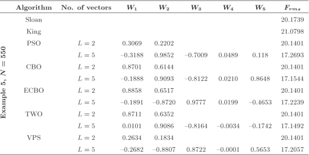
shear wall with 550 nodes is considered. The element clique graph of this model is shown in Figure 10. The performance of the algorithms is tested by this model for prole and wavefront reduction problems. The results are given in Tables 9 and 10, respectively. Example 6. The element clique graph of a rectan-gular FEM with four openings, as shown in Figure 11, contains 760 nodes. The performances of PSO, CBO, ECBO, TWO, and VPS algorithms are tested by this model for prole and wavefront reduction problems. The results for these problems are represented in Tables 11 and 12, respectively.

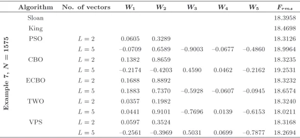
Example 7. The grid model of a fan with 1 D beam elements containing 1575 nodes is considered, as shown in Figure 12. Similar to the previous examples, the obtained values by the algorithms for prole and wavefront reduction problems are given in Tables 13 and 14, respectively, where the results can easily be compared.

Figure 12. The graph model of a fan.

Figure 13. Finite element grid model of a shear wall.

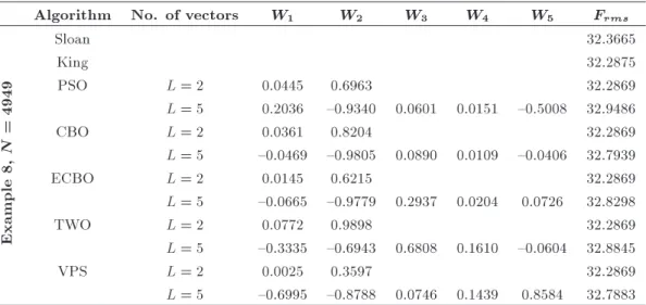
Example 8. The graph model of an H-shaped shear wall with 4949 nodes is considered, as shown in Figure 13. The performance of the above-mentioned algorithms is veried by this model, and the results of these algorithms for prole and wavefront reduction problems are provided in Tables 15 and 16, respectively. 5. Concluding remarks

The main aim of this study is to use VPS algorithm for prole and wavefront reduction of nite element mesh matrices for the rst time and to present the pseudo codes for CBO, ECBO, TWO, and VPS algorithms. The results of these algorithms, when applied to 8 real-life nite element models, were then compared. According to Tables 1 to 16, it can be observed that the achieved results of these algorithms were quite satisfactory, compared to the well-known graph theoretical method of the King and Sloan.

(11)

Table 9. Comparison of the results of prole reduction for the shear wall problem.

Example

5,

N

=

550

Sloan 10530

King 10974

PSO L = 2 0.0007 0.4852 10501

L = 5 {0.0863 0.4638 {0.3677 0.0034 0.9191 9280

CBO L = 2 0.0043 0.4001 10501

L = 5 0.2191 0.9551 {0.6962 {0.0390 {0.3207 9242

ECBO L = 2 0.0001 0.9881 10501

L = 5 {0.0255 0.8883 {0.6256 {0.0110 {0.9183 9237

TWO L = 2 0.0129 0.7645 10501

L = 5 {0.0404 0.8801 {0.5940 {0.0063 0.7426 9237

VPS L = 2 0.0024 0.4913 10501

L = 5 {0.0917 0.9658 {0.6458 {0.0017 0.2137 9237 Table 10. Comparison of the results of wavefront reduction for the shear wall problem.

Example

5,

N

=

550

Sloan 20.1739

King 21.0798

PSO L = 2 0.3069 0.2202 20.1401

L = 5 {0.3188 0.9852 {0.7009 0.0489 0.118 17.2693

CBO L = 2 0.8701 0.6144 20.1401

L = 5 {0.1888 0.9093 {0.8122 0.0210 0.8648 17.1544

ECBO L = 2 0.8858 0.6517 20.1401

L = 5 {0.1891 {0.8720 0.9777 0.0199 {0.4653 17.2239

TWO L = 2 0.8711 0.6352 20.1401

L = 5 0.0101 0.9086 {0.8164 {0.0034 {0.1742 17.1492

VPS L = 2 0.2634 0.1834 20.1401

L = 5 {0.2682 {0.8807 0.8722 {0.0001 0.5653 17.2057 Table 11. Comparison of the results of prole reduction for the rectangular FEM with a four-opening problem.

Example

6,

N

=

760

Sloan 18719

King 18839

PSO L = 2 0.6645 0.9066 18690

L = 5 0.1056 0.8858 {0.4835 {0.0152 0.0524 17136

CBO L = 2 0.1899 0.2566 18689

L = 5 {0.3332 {0.7097 0.9412 0.0507 0.9747 17122

ECBO L = 2 0.6665 0.9228 18581

L = 5 {0.0458 0.7835 {0.6332 0.0060 {0.2254 17039

TWO L = 2 0.7136 0.9633 18581

L = 5 {0.0178 {0.4092 0.9291 0.0024 {0.5575 17039

VPS L = 2 0.1785 0.2491 18581

(12)

Table 12. Comparison of the results of wavefront reduction for the rectangular with a four-opening problem.

Example

6,

N

=

760

Sloan 25.9092

King 26.6508

PSO L = 2 0.2053 0.3469 25.8411

L = 5 {0.0879 {0.3811 0.8933 0.012 {0.1249 23.5891

CBO L = 2 0.3181 0.5433 25.8438

L = 5 {0.0713 {0.6558 0.9556 0.0095 {0.6861 23.4955

ECBO L = 2 0.1855 0.3155 25.8411

L = 5 {0.1056 0.8982 {0.7698 0.0121 {0.7255 23.4743

TWO L = 2 0.5752 0.9624 25.8438

L = 5 {0.0919 0.9571 {0.6803 0.0130 {0.0568 23.5090

VPS L = 2 0.0287 0.05 25.8438

L = 5 {0.0622 {0.4264 0.9926 0.0086 {0.2518 23.4599 Table 13. Comparison of the results of prole reduction for the fan model.

Example

7,

N

=

1575

Sloan 28703

King 28853

PSO L = 2 0.2588 0.6068 28629

L = 5 {0.2965 0.5407 {0.6326 {0.0214 {0.1835 29674

CBO L = 2 0.2129 0.4426 28608

L = 5 {0.5700 0.8618 {0.5831 0.0777 0.3363 27992

ECBO L = 2 0.1765 0.9272 28587

L = 5 {0.4186 0.9776 {0.7792 0.1007 {0.0557 27982

TWO L = 2 0.1613 0.8465 28579

L = 5 {0.3306 0.8144 {0.5654 0.0668 0.6810 27977

VPS L = 2 0.0274 0.1543 28568

L = 5 {0.6613 0.8839 {0.637 0.149 {0.2288 27982 Table 14. Comparison of the results of wavefront reduction for the fan model.

Example

7,

N

=

1575

Sloan 18.3958

King 18.4698

PSO L = 2 0.0605 0.3289 18.3126

L = 5 {0.0709 0.6589 {0.9003 {0.0677 {0.4860 18.9964

CBO L = 2 0.1382 0.8659 18.3235

L = 5 {0.2174 {0.4203 0.4590 0.0462 {0.2162 19.2531

ECBO L = 2 0.1688 0.8892 18.3232

L = 5 0.1883 0.7370 {0.5928 {0.0607 {0.0945 18.6574

TWO L = 2 0.0357 0.1982 18.3240

L = 5 0.0441 0.9101 {0.7696 0.0139 {0.6153 18.0211

VPS L = 2 0.0597 0.3524 18.3168

(13)

Table 15. Comparison of the results of prole reduction for the H-shape problem.

Example

8,

N

=

4949

Sloan 157457

King 157103

PSO L = 2 0.0449 0.6963 157095

L = 5 0.1106 0.9323 {0.0624 {0.0284 {0.3706 160705

CBO L = 2 0.0229 0.9146 157095

L = 5 {0.9709 {0.9856 0.1853 0.2102 {0.3565 159681

ECBO L = 2 0.0620 0.9365 157095

L = 5 {0.5805 {0.7778 0.2437 0.1277 {0.1065 159676

TWO L = 2 0.0721 0.9800 157095

L = 5 {0.8206 -0.8691 0.5953 0.4801 0.2781 159675

VPS L = 2 0.0081 0.8161 157095

L = 5 {0.8685 {0.9894 0.0888 0.1738 {0.1293 159638 Table 16. Comparison of the results of wavefront reduction for the H-shape problem.

Example

8,

N

=

4949

Sloan 32.3665

King 32.2875

PSO L = 2 0.0445 0.6963 32.2869

L = 5 0.2036 {0.9340 0.0601 0.0151 {0.5008 32.9486

CBO L = 2 0.0361 0.8204 32.2869

L = 5 {0.0469 {0.9805 0.0890 0.0109 {0.0406 32.7939

ECBO L = 2 0.0145 0.6215 32.2869

L = 5 {0.0665 {0.9779 0.2937 0.0204 0.0726 32.8298

TWO L = 2 0.0772 0.9898 32.2869

L = 5 {0.3335 {0.6943 0.6808 0.1610 {0.0604 32.8845

VPS L = 2 0.0025 0.3597 32.2869

L = 5 {0.6995 {0.8788 0.0746 0.1439 0.8584 32.7883

In prole and wavefront reduction problems with L = 2 and 5 methods, an attempt was made to display the applicability of using dierent priority functions by utilizing CBO, ECBO, TWO, and VPS algorithms. Optimal weights for these functions were achieved in the optimization processes for reducing the prole and wavefront of the stiness matrices of the nite element models. According to Tables 1 to 16, it can be observed that Sloan and King's approaches can improve in most cases using some new parameters and weights. The weights obtained for dierent examples show that, compared to Sloan and King's algorithms, more suitable prole and wavefront values can be achieved by using the two-parameter method (L = 2). Compared to the two-parameter method and Sloan and King's algorithms, smaller prole and wavefront values can be attained in the ve-parameter scheme (L = 5). However, for Example 8, the values of prole and wavefront of the Sloan and King's methods are smaller than those of the ve-parameter algorithm.

It should be noted that, in L = 5 approach, the active degrees are not updated as in Sloan's technique. Therefore, one should not always expect a better result when ve adjusted parameters are employed instead of two free parameters. Since the graph properties employed in L = 5 method are more than those in L = 2 approach, the amount of reduction in prole and wavefront is higher than that in the Sloan and King's algorithms. The comparison results of the prole and wavefront reduction problem for Example 4 are shown in Figures 14 and 15, respectively.

The new recently developed metaheuristic algo-rithm, namely the vibrating particles system, has been employed in this study for the rst time. Tables 1 to 16 demonstrate that this algorithm nds superior optimal values for prole and wavefront of most of the investigated problems. Moreover, the optimized results obtained by TWO and VPS can compete in performance with those obtained by the other three optimization methods of PSO, CBO, and ECBO and

(14)

Figure 14. Comparison of prole results for Example 4.

Figure 15. Comparison of the wavefront results for Example 4.

Figure 16. Convergence curves obtained for Example 4.

attain better results in some cases. Figures 16-17 and Figures 18-19 show the convergence rate comparisons of these algorithms for prole and wavefront reduction in the case of Examples 4 and 6, respectively.

It should be mentioned that the optimization proposed in this paper was performed to improve the coecients of Sloan's algorithm and was not necessarily limited to the prole reduction of sparse matrices. A direct optimization may or may not result in better values for the prole of the models.

Although the methods of this paper are used for nodal ordering in the stiness method, their application

(15)

can easily be extended to ordering the self-equilibrating systems in the force method.

References

1. Kaveh, A. \Applications of topology and matroid theory to the analysis of structures", Ph.D. Thesis, Imperial College of Science and Technology, London University, UK (1974).

2. Kaveh, A., Structural Mechanics: Graph and Matrix Methods, Research Studies Press, 3rd edition, Somer-set, UK (2004).

3. Kaveh, A., Optimal Structural Analysis, John Wiley, 2nd Edn., Chichester, UK (2006).

4. Papademetrious, C.H. \The NP-completeness of band-width minimization problem", Comput. J., 16, pp. 177-192 (1976).

5. Gibbs, N.E., Poole, W.G., and Stockmeyer, P.K. \An algorithm for reducing the bandwidth and prole of a sparse matrix", SIAM J. Numer. Anal., 12, pp. 236-250 (1976).

6. Cuthill, E. and McKee, J. \Reducing the bandwidth of sparse symmetric matrices", Proceedings of the 24th National Conference ACM, Bradon System Press, NJ, pp. 157-172 (1969).

7. Bernardes, J.A.B. and Oliveira, S.L.G.D. \A sys-tematic review of heuristics for prole reduction of symmetric matrices", Procd. Comput. Sci., 51, pp. 221-230 (2015).

8. King, I.P. \An automatic reordering scheme for simul-taneous equations derived from network systems", Int. J. Numer. Methods Eng., 2, pp. 523-533 (1970).

9. Kaveh, A. and Behzadi, A.M. \An ecient algorithm for nodal ordering of networks", Iran. J. Sci. Tech-nol., Transactions in Civil Engineering, 11, pp. 11-18 (1987).

10. Kaveh, A. and Roosta, G.R. \Comparative study of nite element nodal ordering methods", Eng. J., 20(1&2), pp. 86-96 (1998).

11. Koohestani, B. and Poli, R. \Addressing the envelope reduction of sparse matrices using a genetic program-ming system", Comput. Optimiz. Appl., 60, pp. 789-814 (2014).

12. Kaveh, A., Advances in Metaheuristic Algorithms for Optimal Design of Structures, 2nd Edn., Springer International Publishing, Switzerland (2017).

13. Kaveh, A. and Mahdavi, V.R. \Colliding bodies op-timization: A novel meta-heuristic method", Comput. Struct., 139, pp. 18-27 (2014).

14. Kaveh, A. and Ilchi Ghazaan, M. \Enhanced colliding bodies optimization for design problems with continu-ous and discrete variables", Adv. Eng. Softw., 77, pp. 66-75 (2014).

15. Kaveh, A. and Zolghadr, A. \A novel meta-heuristic algorithm: tug of war optimization", Int. J. Optim. Civil Eng., 6, pp. 469-492 (2016).

16. Kaveh, A. and Ilchi Ghazaan, M. \A new meta-heuristic algorithm: vibrating particles system", Sci. Iran., 24(2), pp. 551-566 (2017).

17. Sloan, S.W. \An algorithm for prole and wavefront reduction of sparse matrices", Int. J. Numer. Methods Eng., 23, pp. 1693-1704 (1986).

18. Kaveh, A. and Rahimi Bondarabdy, H.A. \A hybrid method for nite element ordering", Comput. Struct., 80(3-4), pp. 219-225 (2002).

19. Rahimi Bondarabady, H.A., and Kaveh, A. \Nodal ordering using graph theory and a genetic algorithm", Finite Elem. Anal. Des., 40(9-10), pp. 1271-1280 (2004).

20. Kaveh, A. and Shara, P. \Optimal priority functions for prole reduction using ant colony optimization", Finite Elem. Anal. Des., 44, pp. 131-138 (2008).

21. Kaveh, A. and Shara, P. \Ordering for bandwidth and prole minimization problems via charged system search algorithm", Iran. J. Sci. Technol., Transactions in Civil Engineering, 36(C1), pp. 39-52 (2012).

22. Kaveh, A. and Bijari, Sh. \Bandwidth, prole and wavefront optimization using PSO, CBO, ECBO and TWO algorithms", Iran. J. Sci. Technol., Transactions in Civil Engineering, 41(1), pp. 1-12 (2017).

23. Everstine, G.C. \A comparison of three resequencing algorithms for the reduction of matrix prole and wavefront", Int. J. Numer. Methods Eng., 14(6), pp. 837-853 (1979).

Biographies

Ali Kaveh was born in 1948 in Tabriz, Iran. After graduation from the Department of Civil Engineering at the University of Tabriz in 1969, he continued his studies on Structures at Imperial College of Science and Technology at London University and received his MSc, DIC, and PhD degrees in 1970 and 1974, respectively. He then joined the Iran University of Science and Technology. Professor Kaveh is the author of 625 papers published in international journals and 155 papers presented at national and international conferences. He has authored 23 books in Farsi and 8 books in English published by Wiley, RSP, American Mechanical Society, and Springer.

Shima Bijari is a PhD candidate in Civil Engineering Department of Iran University of Science and Technol-ogy. She took a BSc degree in 2012 and MSc in 2014. Her main expertise and experience reside in the eld of structural engineering and optimal design of structures. She is interested in metaheuristic algorithms and their applications.