2440.pdf

Subgroup Variation in Diagnostic Tests: Sources

and Solutions

By

Daniel Nissman

A Master's Paper submitted to the faculty of the University of North

Carolina at Chapel Hill in partial fulfillment of the requirements for

the degree of Master of Public Health in the Public Health Leadership

Program

Chapel Hill

Subgroup Variation in Diagnostic Tests: Sources

and Solutions

Daniel Nissman

Abstract

Diagnostic tests are an essential component of clinical medicine today.

Like any other clinical study, the results of studies evaluating new diagnostic tests

must be interpreted in the context of underlying methodological problems and

generalizability. Subgroup variation in diagnostic test accuracy, the focus of this

paper, can arise in two ways: the test truly performs differently in the two

subgroups or it is an artifact. Real subgroup variation affects the generalizability

of the results. Artifacts, however, arise from biased measurement (e.g. an

imperfect reference standard) and affect the believability of the results. The

question is whether real subgroup variation can be separated from artifact.

Sources of subgroup variation and examples are presented with the

specific focus on true subgroup variation and spurious variation due to the use of .

imperfect reference standards. Both true variation and the use of imperfect

reference standards are shown to be quite common. Frequently used tests, such as

the urine dipstick for urinary tract infection, exhibit true subgroup variation.

Observed test characteristics derived from comparison to an imperfect reference

are shown to be prevalence-dependent. The effect of measurement reliability is

discussed as a third source of potential subgroup variation.

Two basic approaches for managing imperfect reference standards are

references. The emphasis is on the method ofHui and Walter, which provides a

closed form expression for identifYing the unknown characteristics of the new test

and the reference test in two populations. An alternate derivation is also provided

that may be more accessible to the non-statistician.

Methods for identifying true subgroup variation, simple stratification and

regression analysis, as well as methods for incorporating subgroup variation into

clinical decision making are presented to round out the general discussion of

subgroup variation. IdentifYing subgroup variation and accounting for covariates

in diagnostic test parameters is not significantly different from similar analyses in

studies of interventions. The use of likelihood ratios to measure the impact of

subgroup variation on decision making as well as a means for mitigating poor

generalizability ("spectrum bias") of a test when used in a population with a

different severity of disease completes the discussion.

The paper is concluded with a methodology for distinguishing true

subgroup variation from spurious subgroup variation due to an imperfect

reference standard.

I

Introduction

Diagnostic tests are an essential component of clinical medicine today.

Like any other clinical study, the results of studies evaluating new diagnostic tests

must be interpreted in the context of underlying methodological problems and

generalizability. Subgroup variation in diagnostic test accuracy can arise in two

Real subgroup variation affects the generalizability of the results. Artifacts,

however, arise from biased measurement (e.g. an imperfect reference standard)1

and affect the believability of the results. The question is whether real subgroup

variation can be separated from artifact.

Imperfect reference standards are a common problem2 Pathologists are

not 100% accurate and they may have reporting preferences dictated by where

they trained. Bacterial culture, a frequently used reference, is not 100% sensitive.

Pulmonary angiography for pulmonary embolism is not 100% sensitive. Under

idealized circumstances, the use of an imperfect reference results in

underestimation of one or both of a test's sensitivity, the proportion of diseased

cases that test positive, and specificity, the proportion of non-diseased cases that

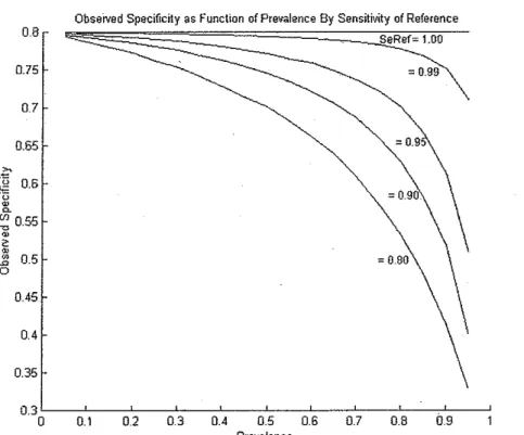
test negative. First noted by Gart and Buck in 1966/ the effect on the observed

test characteristics is dependent on disease prevalence. See Figures 1 and 2. If

the performance characteristics of the imperfect reference are known, then the

new test's characteristics can be corrected algebraically. 4

When a test performs differently in two subgroups leading to different test

characteristics in the two groups, the test is said to exhibit "spectrum effect" or

"spectrum bias. "5 Diagnostic testing studies usually report the results for the

entire study sample leading to a weighted average of the sensitivities and

specificities for each of the subgroups. This is inappropriate as the weighted

average no longer applies to either group. In some cases, clear biological

differences can explain differential test performance. Tests relying on antibody

(decreased sensitivity). Similar tests performed in patients with autoimmune

diseases experience greater risk for antibody cross-reactivity, which leads to

decreased specificity.

An imperfect gold standard can mimic spectrum effect when the

prevalence of the disease or condition of interest is different in the subgroups. 1

Inappropriate assigmnent of true case/noncase can greatly affect the computed

performance characteristics of the test under study. This situation may arise when

studying symptomatic versus asymptomatic people. The prevalence of disease is

likely much greater among symptomatic individuals than in asymptomatic

individuals.

0.8

0.75

0.7

0.65 ~

i

~

~ 055 ~ .

~ 2 ro 1? 0.5

0

0.45

0.4

0.35

Obseived Specificity as Function of Prevalence By Sensitivity of Reference SeRef= 1.00

= 0.99

=0.9

0.3 L_---,.L_-:":--:-':---:-'-:---::-':::---::-':---::'::---c-~---,L---"

0 0.1 0.2 0.3 0.4 0.5 0.6 0.7 0.8 09

Prevalence

Figure 1: Observed specificity as a function of prevalence for several values of reference test sensitivity. The test's true specificity in this example is 0.80. As

Obsemd Sensitivity .as Function of Prevalence By Specificity of Reference

08

SpRef"' 1.00

075 .. Q_gg

0.7

= 0.95 0.65

0.45

0.4

0.35

0.3L--~--'---~-~--'---'---~--'---'--~

0 0.1 0.2 0.3 0.4 0.5 0.6 0.7 0.8 0.9

Prevalence

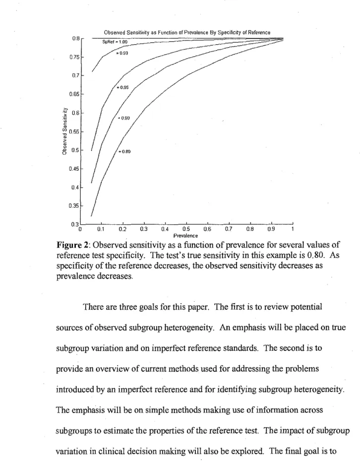
Figure 2: Observed sensitivity as a function of prevalence for several values of reference test specificity. The test's true sensitivity in this example is 0.80. As specificity of the reference decreases, the observed sensitivity decreases as prevalence decreases.

There are three goals for this paper. The first is to review potential

sources of observed subgroup heterogeneity. An emphasis will be placed on true

subgroup variation and on imperfect reference standards. The second is to

provide an overview of current methods used for addressing the problems

introduced by an imperfect reference and for identifYing subgroup heterogeneity.

The emphasis will be on simple methods making use of information across

subgroups to estimate the properties of the reference test. The impact of subgroup

variation in clinical decision making will also be explored. The final goal is to

present a methodology for distinguishing true subgroup variation from spurious

II

Background

ll.l

Subgroup Variation

ll.l.l "Spectrum"

The use of the term "spectrum" in relation to biases and population

subgroups when discussing diagnostic tests is confusing. On the one hand, when

used in the phrase "adequate spectrum," it refers to the range of subjects against

which a test should be evaluated to arrive at a single set of test characteristics. On

the other hand, when used in the phrase "spectrum bias" or "spectrum effect," it

implies different test characteristics across subgroups. Subgroup variation among

tests has been recognized at least since the 1970s, yet the systematic exploration

of subgroup variation is still not a component of typical diagnostic test evaluation

studies. An unintended consequence of using the phrase "adequate spectrum,"

which is still a component of all guidelines for diagnostic test evaluations, may be

that subgroup analysis of diagnostic tests is not pursued to the extent they should

be. The following discussion tracks the evolution of the concept of spectrum

from its initial introduction to its current day usage.

Ransohoff and Feinstein first introduced the concept of"spectrum" in

19786 In their usage of the term, diagnostic tests need to be evaluated on a

sufficiently broad "range of features found in patients" to get a more accurate

depiction of the sensitivity and specificity of a test. This broad range should

include a broad range of pathologies, a broad range of symptomatic severity, and

using an inappropriate spectrum during the development or study of a test are that

the test performs poorly in practice.

Subsequently, in 1988, Miller, et al} subdivided Ransohoff and

Feinstein's "spectrum" into selection bias and "disease-based spectrum." In

selection bias, there is a spurious association between a patient characteristic and

the diagnosis of interest. In "disease-based spectrum" bias, a restricted range of patients is recruited into a study based on an intermediate to high probability of

disease. In other words, selection is based on a restricted range of disease severity. An example of such bias is the selection of patients for angiography.

These patients have already received several tests indicating a significant

likelihood for coronary artery disease (CAD). Generalization of test

characteristics derived from populations exhibiting these biases will be poor.

In 1990, the term "spectrum bias" was first used by Nardone, et al} to

refer to the use of an inappropriate spectrum of patients in past studies of the

diagnosis of anemia by skin pallor. In this case, an inappropriate spectrum appears to have been any study that did not have equal numbers of anemic and

normal patients. Although this is not exactly what Ransohoff and Feinstein meant

by appropriate spectrum, they did go to great lengths to design a study with equal

proportions of patients in 5 different hematocrit ranges. They find that the

sensitivity of skin pallor was greater the lower the hematocrit, which corroborates

many subsequent findings that test sensitivity is greater the more severe the

In 1992, Lachs, et al., 9 first associate the term "spectrum bias" with

different test characteristics in a pair of subgroups. In this study of diagnosis of

urinary tract infection by urine dipstick, the aggregate sensitivity and specificity

was found to be 83% and 71%, respectively. When divided into groups based on

high versus low pretest probability, the sensitivity and specificity was found to be

92% and 42%, respectively, in the high probability group and 56% and 78%,

respectively, in the low probability group. This paper is the firstto note caution

when aggregating test characteristics among subgroups. Unfortunately, they also

state that "spectrum bias will not produce misleading appraisal of test

performance if the groups recruited for the study are representative of the patients

in whom it will ultimately be used in clinical practice." This is incorrect because

there may be subgroup variation within the typical range of clinical practice

patients. An example of subgroup variation that is cited in their article that is

counter to their statement is the use of exercise stress testing for coronary

ischemia in men and women. Sensitivity of exercise stress testing for coronary

ischemia in men is 72.4% and in women it is 57.2%; 10 and, for the presence of

coronary artery disease, the sensitivity is 63.5% in men and only 29% in

women.11

Finally, in 2002, Mulherin and Miller5 refer to the variation of test

characteristics among subgroups as "spectrum effect." They argue that this is not

a systematic bias that needs to be controlled against. Rather, this is an example of

effect modification- the diagnostic test simply performs differently in different

Characteristics for each subgroup in which variation is found should be reported

separately.

The concept of appropriate spectrum in diagnostic tests as described by

Ransohoffand Feinstein's definition of spectrum as "the range of features found

in patients used to challenge a test's sensitivity and specificity"6 (p. 927) to be

reported as a single set of characteristics is now supplanted by the need for the

consideration of variation in test characteristics among subgroups. Although

subgroup differences have been recognized in the diagnostic testing literature for

specific tests (see Table 1), the formal discussion of the spectrum effect provides

a framework to explore subgroup variation in all diagnostic tests. The

consequence of this, however, is that greater effort must be made at adequate

representation of subgroups of interest in evaluation studies.

A further point regarding spectrum needs to be made. There are two

components to the evaluation of a diagnostic test prior to its introduction to

general use6 First, in evaluating the sensitivity of the test it is important to

provide adequate examples of disease across its many manifestations and in the

presence of co morbid conditions. Second, as many mimics of the condition of

interest as possible need to be presented to the test to properly evaluate the test's

specificity. It is inappropriate to only evaluate the specificity in a population of

normal individuals. (A possible exception to this is when the test is used for

screening purposes.) The concept of a broad range of evaluation conditions is the

original concept of spectrum as defined by Ransohoff and Feinstein. However,

range of manifestations or comorbid conditions and that this behavior should be

explicitly reported has only recently been formally recognized.

Ultimately, designing and evaluating studies of diagnostic tests should be

no different from designing intervention studies. In the classic 1987 paper by

Colin Begg, 12 he states that "it may seem anachronistic to caution statisticians to

consider adjustment for covariates ... given that covariate adjustment has been a

major topic of study in statistics for much of this century. However, in the

majority of test efficacy studies the issue is not addressed."(p 413l Consideration of

covariates, i.e. subgroups, is increasing, albeit slowly. Like intervention studies,

consideration of selection bias, subgroup analysis, and generalizability should be

fundamental aspects of study design and critical appraisal.

11.1.2 Examples

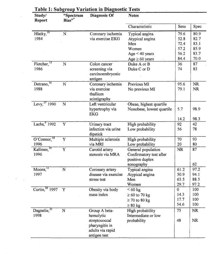
Table !lists all studies of diagnostic tests identified by searches on

"spectrum bias" and "spectrum effect" on PubMed. (There is no MeSH term for

this concept.) Included in this table are examples of other diagnostic testing

modalities reporting subgroup variation. A key point from examination of this

table is the presence of significant subgroup variation in frequently used tests.

Urine dipsticks and the rapid antigen test for "strep throat" are frequently used

tests in emergency departments and primary care offices. Electrocardiograms are

also frequently obtained. With the high prevalence of obesity today,

understanding that body mass index (BMI) does not perform well for people less

one editorial14 that specifically mention "spectrum bias," but got the definition

incorrect, are included in the list.

Table 1: Subgroup Variation in Diagnostic Tests Study/ "Spectrum Diagnosis Of Notes Report Bias""

Characteristic Sens Spec

Hlatky,'" N Coronary ischemia Typical angina 79.6 80.9 1984 via exercise EKG Atypical angina 52.8 82.7

Men 72.4 83.1

Women 57.2 85.9

Age < 40 years 56.2 83.7 Age > 60 years 84.4 70.0 Fletcher," N Colon cancer Duke A orB 36 87

1986 screening via Duke CorD 74 83

carcinoembryonic

antigen

Detrano,16 N Coronary ischemia PreviousMI 95.6 NR

1988 via exercise No previous MI 79.1 NR

thallium scintigraphy

Levy,'' 1990 N Left ventricular Obese, highest quartile

hypertrophy via Nonobese, lowest quartile 5.7 98.9 EKG

14.2 98.3 Lachs,' 1992 y Urinary tract High probability 92 42

infection via urine Low probability 56 78 dipstick

O'Connor," y Multiple sclerosis High probability 70 93

1996 viaMRI Low probability 20 80

Kallmes," y _{Carotid artery General population NR} 87 1996 stenosis via MRA Confirmatory test after

positive duplex

sonography 62

Moons," N Coronary artery Typical angina 61.2 97.2 1997 disease via exercise Atypical angina 50.9 94.1 stress test Men 63.5 88.5

Women 29.7 97.2

Curtin,'" 1997 y Obesity via body <60kg 0 100

mass index <: 60 to 70 kg 14.3 100

<: 70 to 80 kg 17.7 100

<: 80 kg 54.6 100

Dagnelie," N Group A beta- High probability 75 NR

1998 hemolytic Intermediate or low

streptococcal probability 48 NR

Study/

Report

Barnhart, 14 1999

Colin, 22 2000

DiMatteo," 2001 Mulherin/ 2002 Huot," 2002 ,,

Lim, 2003

Hall," 2004

"Spectrum Diagnosis Of Bias"'"

Y Infertility via FSH

Y Hepatitis C via 'b d I

anti o y sera ogtes

(RIBA 3'• generation)

y Group A beta-hemolytic streptococcal pharyngitis in adults via rapid antigen test

y _Chlamydia

· trachomatis

infection via

enzyme immunoassay

y _{Renal artery} stenosis via

captopril renal scan

..

Y Cogmllve

impairment via two questionnaires

Y Group A beta-hemolytic streptococcal pharyngitis in children via rapid antigen test NR - not reported.

'study explicitly mentions "spectrum bias."

Notes

Characteristic

I

I

Qualitative consideration of antibody tests

. d. d' 'd I

m tmmunocompromtse m tvt ua s

Chronic liver disease 100 100 Hemodialysis

79 100 Modified Centor criteria:

0,1

2 61 NR

3 76

4 90

97

Age<24 75.9 99.5 Age;e24 58.3 99.2

With vascular disease

Without vascular disease 70 63

100 55 Different performance between two

screening instruments on same group

erroneously attributed to spectrum bias Modified Centor criteria:

0

I 47 NR

2 65

3,4 82

90

Two further areas of intense clinical interest where subgroup variation is

present are in the early detection of breast cancer via screening mammography

and in the diagnosis of pulmonary embolism (PE) via pulmonary angiography

and, possibly, the D-dimer assay. There has been a significant amount of

mammography is lower among younger women than in older women. In

pulmonary angiography, whether by computed tomography ( CT) or magnetic

resonance (MR), there is a clear difference in the ability of these techniques to

detect large vessel emboli and subsegmental emboli. 32•33.34.35

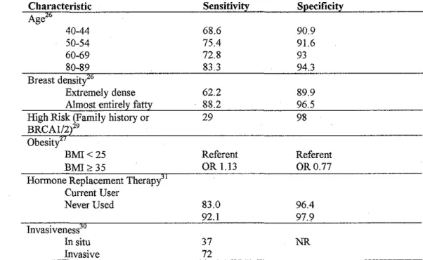
Table 2: Examples of Subgroup Variation in the Performance of Screening Mammography

Characteristic Sensitivity Specificity

Age26

40-44 68.6 90.9

50-54 75.4 91.6

60-69 72.8 93

80-89 83.3 94.3

Breast densi

Extremely dense 62.2 89.9 Almost entirely fatty 88.2 96.5 High Risk (Family history or 29 98 BRCAI/2 29

Obesity

BMI<25 Referent Referent

BMI>35 OR l.l3 OR0.77

Hormone Replacement Therapy" Current User

Never Used 83.0 96.4

92.1 97.9

Invasiveness

In situ 37 NR

Invasive 72

Considerable attention has been given to subgroup variation in the

screening mammography literature. Table 2 provides examples of published

variations in test characteristics among subgroups and is not meant to be an

exhaustive synthesis of the available data on each of the listed subgroups.

Conflicting data do exist, especially regarding the effect of hormone replacement

therapy,26•31 so the data serves for illustration only. As is common in studies of

interventions, some identified subgroups may in fact be proxies for other

b

'

underlying characteristics. For example, age is most likely a proxy for breast

density. What is important is that subgroup variation is being explored, because

clinically important subgroups exist. In particular, mammography does not

perform well at all in women who are at high risk of breast cancer compared to

the woman at average risk.

The diagnosis ofPE is also subject to subgroup variation. In this case, subsegmental emboli seem to represent a different entity. Many may actually

represent incidental findings and, if truly associated with the event, do not carry

the same clinical significance that an embolism found in a larger pulmonary

vessel would have in the near term. 36•37 Regardless of this fact, angiographic

methods have difficulty with detecting emboli in the smaller vessels. The reason

for this difficulty is due to a combination of motion artifact and poor spatial

resolution.· Since fluoroscopic pulmonary angiography is the de facto gold

standard, one can only discuss inter-rater variability when discussing its accuracy.

Stein, et al.,32 using the degree of co-positivity between two observers, found that

co-positivity for presence of an embolus in a subsegmental artery was 66%

compared to a co-positivity of 90% and 98% in the segmental and central or lobar

arteries, respectively. For single-slice CT, Goodman, et al.,32 found a sensitivity

of 86% in the central arteries and only 25% in the subsegmental arteries for the

diagnosis ofPE. Modern multislice CT scanners perform significantly better and

are able to visualize the subsegmental arteries twice as well as single-slice

with the smaller vessels, has reported sensitivities of 40% for subsegmental, 84%

for segmental and 100% for central or lobar PE. 35

According to the study by De Monye, et al.,38 the D-dimer test for PE also

displays subgroup variation by location. The test had a sensitivity of93% for PE

located in the segmental or larger arteries and a sensitivity of only 50% when the

embolism was located in the subsegmental arteries. The D-dimer assay has good

performance for ruling out large vessel PE, but relatively poor performance for

ruling out smaller emboli. Since this assay is usually only obtained in a patient

with a low clinical suspicion ofPE and an individual with a large vessel PE is

unlikely to be asymptomatic, then a negative test would be falsely reassuring.

Subgroup variation in diagnostic test performance clearly exists for the

tests used for many common problems. The reporting of aggregate test

characteristics across all patients distorts the performance· of the tests in clinically

important subgroups. Hopefully, understanding this variation will lead to more

appropriate use of diagnostic tests, which will ultimately lead to better care for

patients.

ll.1.3 Does This Test Exhibit Subgroup Variation?

When considering the possibility that a subgroup may behave differently

from the larger group that a test is normally used in, there are some clues to

consider. These include biological plausibility and wide variations in published

test characteristics. By understanding the scientific basis for a given test,

erroneous test result. By examining the published literature for a given test, wide

variations in published test characteristics are clues to heterogeneity39 The

heterogeneity may be due to poor study design or it may be due to selection of

different sets or proportions of subjects.

Predicting subgroup variation on the basis oftest mechanism is not

difficult. Tests relying on the detection of antibodies do not perform as well in

people who are deficient in antibodies. Imaging fine anatomical structures, such

as small pulmonary arteries, will be difficult if the patient moves or if the spatial

resolution of the technique is not adequate. Visualizing abnormalities in dense

breast tissue is more difficult than in fatty breast tissue. On the other hand,

finding subgroup variation may lead one to rethink the disease and/or testing

process. Why does exercise stress testing not perform well in women compared

to men? Why does the rapid antigen test for Group A beta-hemolytic

streptococcal pharyngitis perform better the more severe the disease is?

Heterogeneity between studies of diagnostic tests can be due to a number

offactors: study design and conduct; population (and circumstances) under study;

and choice of reference test. 39 Many biases can be introduced in the conduct of a

diagnostic testing study. Unfortunately, proper design and conduct of diagnostic

testing trials has not received the attention that intervention trials have received.

Today, however, guidelines for the proper design and reporting of these studies

are available40·41 The choice of reference test can lead to different results. For

example, now that fluoroscopic pulmonary angiography is known not to be 100%

CT angiography plus lower extremity venous Doppler ultrasound to improve the

reference standard's sensitivity for diagnosing PE. In many cases, there is likely

to be selection bias in the evaluation of a test, where a particular subgroup is over

(or under) represented. If all other factors are equal, this is a strong clue that there

may be subgroup variation.

Systematic reviews of diagnostic tests are confronted with a particular

difficulty. Diagnostic test performance is reported as two quantities. The usual

tests for heterogeneity rely on the presence of only one quantity of interest. In a

review of the use of tests for heterogeneity in systematic reviews of diagnostic

tests, Dinnes, et a!., note that "the under use of statistical tests and graphical

approaches to identify heterogeneity perhaps reflect the uncertainty in the most

appropriate methods to use ... " 39 (p. iii)_ There is clearly more work that needs to

be done in this area.

As a final caveat, diagnostic tests based on dichotomizing continuous

outcomes may appear to have different test characteristics simply by using a

different threshold.12•39 The receiver operating characteristic (ROC) curve should

be examined in these cases as it provides a description of the separability of the

two classes, diseased and not diseased. If the curve is identical, the tests are the

ll.2 Imperfect Reference Standard

ll.2.1 Examples

Imperfect reference standards are common in many aspects of diagnostic

testing. Microbiological testing is an area that has struggled with imperfect

references for many years. Culture is never 100% sensitive. In a comparison of

diagnostic methods for chlamydia] urogenital infection by Biro, et aL,42 culture

sensitivity was in the range of 75% to 80%. Even PCR for detection of viral (or

other organism) RNA is not 100% perfect. The gold standard against which PCR

for hepatitis C virus was evaluated was through inoculation of chimpanzees. 22

Microscopy for the detection of malaria on thick blood smears is considered to be

the gold standard for diagnosing malaria in field trials. Unfortunately, when

compared with expert review, microscopy has a sensitivity of91% and a

specificity of 71%.43

Angiography is another area where imperfect reference standards exist.

Fluoroscopic pulmonary angiography, as noted before, is not perfect at imaging

the smaller pulmonary arteries. Angiography of the renal arteries also does not

have perfect sensitivity. In a study evaluating the accuracy of CT angiography

and MR angiography for the diagnosis of renal artery stenosis, three separate

observers evaluated the fluoroscopically obtained images to arrive at a consensus

diagnosis. 44

Finally, pathological examination of specimens is not 100% sensitive.

Sampling error is an obvious source of false negatives. A less obvious source of

definitions. While most pathologists can agree on the extremes of disease,

borderline cases cause a great deal of difficulty. Interobserver variability can be

quite high in some circumstances. For an interesting discussion with examples,

see the 2003 editorial by LiVolsi45 and the response by Ackerman46 Some

examples: from LiVolsi, agreement as to the benign or malignant nature of a

papillary lesion with a follicular pattern in thyroid tissue is around 50%; and, from

Ackerman, discordance among experts on the diagnosis of a melanocytic

neoplasm ranges from 26% to 80% depending on the panel.

The imperfect gold standard is a common problem in the evaluation of

diagnostic tests. The general effect of using an imperfect reference, especially

when the new test and the reference test are conditionally independent, is to cause

underestimation of the new test's performance. As noted previously, this

underestimation is dependent on the prevalence of disease and may, additionally,

produce spurious subgroup variation when subgroups have different prevalences

of disease.

II.2.2 . Is This Reference Test Imperfect?

When evaluating a test as a possible reference or when appraising an

article on a diagnostic test, there are some clues that may be useful in evaluating

the quality of the reference. Since there is no comparison for a "gold standard"

test, two features of a test may indicate less than perfect performance in practice.

First, if there is interobserver variation in the interpretation of the test, especially

to be perfect Second, if adjudication of the test requires differentiation of

borderline cases or requires grading on a continuum divided by a threshold, then

the test is unlikely to be perfect Many radiological and pathological tests suffer

both from interobserver variability and dichotomization of continua. Any test

making use of a human observer should be subject to considerable scrutiny. A

third category is the use of composite reference standards. Composite references

are composed of imperfect reference tests, which rarely make a perfect reference

in the aggregate.

ll.3 Measurement Error

The role of measurement error on subgroup heterogeneity will be

mentioned here. For tests based on dichotomization of a continuous measure,

measurement error causes degradation of test performance47'48 Confusion exists,

however, regarding the dependence of this performance degradation on

prevalence. In 1997, Brenner and Gefeller published a provocative paper that

suggested significant variation of sensitivity, specificity, positive predictive value,

and negative predictive value in the presence of noise with disease prevalence. 48

In a letter to the editor, Bender, et al., 49 took issue with their stance, arguing that

the model system in which Brenner and Gefeller arrived at their results was

outside the paradigm of what is normally considered to be "diagnostic testing"

and would be misleading to the clinicians making use of these tests. For the

traditional diagnostic testing paradigm, where test characteristics are evaluated

should not be related to prevalence. To paraphrase Brenner and Gefeller, they

would rebut by saying that many more diagnostic decisions are made based on

subdividing a single distribution of some characteristic in the population into

"diseased" versus "not diseased" .and that noise can have profound effects on test

performance as a function of prevalence. Furthermore, they argue that diagnostic

decision theory, as a field, needs to come to terms with this effect. As it turns out,

both points-of-view are correct. What follows is an illustration of how

measurement noise affects test characteristics under the two paradigms.

ll.3.1 Measurement Reliability

To provide a framework for discussing measurement noise, the concept of

measurement reliability is discussed here. An inherent amount of variation is

present in any measurement. This variation may be intrinsic to the process being

measured or it may reflect variation in the population and is typically accounted

for in descriptions of how this continuous measure varies in the population.

Unwanted variation, however, whether due to environmental conditions (e.g., heat

exposure during transport), observer variation, or other factors, can degrade the

reliability of one's measurement. Statistically, measurement reliability, p, is

conceptualized as the proportion of the variance due to the intrinsic processes,

cri

over the total variance,

cr?

cr/,

cr/

measurement error: p =

cr?/(cr?

measurements. Low reliability coefficients indicated that unwanted variance

contributes significantly to the overall variance of observed measurements.

Measurement error does not only arise from unwanted environmental

intrusions, inherent limitations of laboratory equipment, or variations among

observers. Application of a measurement system with a particular underlying

assumption about the distributions of interest to a population with a different set

of distributions can also result in a significant degradation of the reliability of

one's measurements. When spectrum bias is viewed in terms of measurement

reliability, application of a test in a population in which the test was not evaluated

can result in a significant reduction in the reliability of the result.

The simulations presented in the next two sections make use of

measurement reliability to illustrate the effects of measurement error on test

performance. As a point of reference, a good reliability for laboratory tests is

ll.3.2 Two-Distribution Paradigm 018 0.16 0.14 -~0-12 • c ~ 0.1 D ~ .~

~ 0.08 -g

0: 0.06 Non-diseased +Noise ~

004

~/

~ ~

002 ~

Distribution ofT est Results for Diseased And Non-Diseased Individuals

Non-diseased

---

~... Diseased + Noise

--- I

---

~~-~~--6 8 10 12 18 . 20

Continuous Test Result

Figure 3: Two-distribution paradigm. Distributions of a continuous test result

for both diseased and non-diseased individuals are shown (solid lines). The addition of noise causes a broadening of the distributions (dotted lines). The ·increased overlap leads to increased false negatives (more area under the curve to

the left of the threshold for the diseased + noise distribution when compared to the diseased without noise distribution) and increased false positives (more area under the curve to the right of the threshold for the non-diseased + noise distribution when compared to the non-diseased without noise distribution).

In classic diagnostic testing, test characteristics are derived by comparing

the results of a test to a gold standard. In this case, the distributions of values for

a particular measure are known and separate for both diseased and healthy

individuals. Since two distributions are involved, I have termed this the

"two-distribution paradigm."

Selection of a decision threshold, and its position relative to the two

distributions, determines the sensitivity and specificity of the test. The addition of

noise affects each distribution separately. Noise typically adds variance to any

diseased individuals and the location of a threshold, sensitivity is only affected by

alterations of the distribution. The relative number of samples of a population

from the diseased distribution does not affect this process. Thus, sensitivity is not

dependent on prevalence. The same is true for specificity.

Figure 3 illustrates distribution functions for diseased and non-diseased

individuals and then, superimposed, the same distributions with noise added in.

By examining the graphs, one can see that the number of false positives and false

negatives are increased in the presence of noise. The probability of this occurring

is only dependent on whether the subject is diseased or non-diseased. The actual

number in a sample does not affect this probability. Therefore, noise degrades

performance in this paradigm, but it is not dependent on the prevalence of disease.

Figure 4 shows the ROC curve for varying levels of measurement reliability.

ROC CuJVe

OL---~--~~

0 0.2 0.4 0.6 0.8

False Posrtive Fraction (1 - specificity)

Test Characteristic Versus Reliability Coefficient

0.9,----~---,

<.> 0.85

~ 1~

t;

~ 0.8 m

.c <.> 1ii

"'

,_ 0.75 .

0.7L_-~---~--'

1 0.9 0.8 0.7 0.6

Reliability Coefficient, rho

Figures 5 and 6 show the results of simulations designed to evaluate the

effect of prevalence on test characteristics at varying levels of measurement

reliability. The distributions are both normal with variance 4. The mean of the

non-diseased distribution is 6 and the mean of the diseased distribution is I 2. The

simulation was run for six values of p, ranging from 0.1 to 1.0, and 19 values of

prevalence, ranging from 0.05 to 0.95 at 0.05 increments. Two hundred thousand

subjects contributed to the estimates at each data point. Variance of the noise in

F . _tgure 5 . _{IS COmpute} d _{as O"noise -}2 - ( _{O'comb -}2 _p

*

+ 0diseasel To investigate the effect of differential noise, which, for example, is

seen with blood pressure measurements, 50 the simulations were run again (Figure

6) using different quantities of noise for measurements drawn from the

non-diseased and non-diseased distributions. Since variance is additive, the noise variance

derived above was divided among the two populations proportional to their

means: Onoise; non-diseasel = )lnon-diseased

*

disease/ = J.ldiseased

*

prevalence has no effect on test characteristics even in the prevalence of noise. In

the simulation involving differential noise, we note that sensitivity is degraded

more by decreasing reliability than specificity as it was affected by a greater

Sensitivity vs. Prevalence By Reliability

0.95 P"" LO 0.95

0.9 _..-·----~~~--- p=0.9 _0.9

·-"' 0.85 >

:lii 0.8

0

ID

r.n 0.75

0.7

---~---~

/'---·--·

p = 0.1 :>.. 0.85

:~

p=0.5 ~ 0.3

~ ~

p=0.3 ({.1 0.75

0.7

Specificity vs. Prevalence By Reliabillly

---~-.

--~---.

p= 1.0

p=0.9 p-<>0.7

p = 0.5

p =0.3

065

- - - · · p=O.t 0.65 - - - _ , - _ . . . . • , p=O.l

06'---~-~-~----0 0.2 0.4 0.6 0.8 .

06L_ _ _ _ _ _ _ _ _ _

0 0.2 0.4 0.6 0.8

Prevalence Prevalence

Figure 5: Sensitivity versus prevalence for varying levels of reliability. Noise

was applied equally to measurements from diseased and non-diseased individuals. Note that both sensitivity and specificity are degraded equally and without

dependence on prevalence.

0.95 0.9

» 0.85

-~

-~

·~ 0.8

c

00

(/) 0.75 0.7 0.65

Sensitivity vs. Prevalence By Reliability

...

---~---

----~---·-·-·-·-

~,-·-·---~-·-,---

-·-·-·---0.6 ~---::-'::---:Cc---::->::--::"::--~

0 0.2 0.4 0.6 0.8

Prevalence

Specificity vs. Prevalence By Reliability

0.95 p = 1.0

P"'09

p=0.1

0.9 - - - - -- - - - ~

-p "'0.5 » 0.85 'G

1j 0.8

P"'0.3 2;_

(IJ 0.75

---~-~·~·-·-·-'~·-,---,~

p= 1.0

p=0.9 p=0.7

p:0.5

p•0.3

_ . . - - - · - - - · - - · - ' - · - . . , - p=>O.t

0.7

p=O.l

0.65

0.6L_-~-~-:->::--~-~

0 0.2 0.4 0.6 DB

Prevalence

Figure 6: Sensitivity versus prevalence for varying levels of reliability, but with

differential noise. In this model of differential noise, measurements from

diseased individuals experienced greater amounts of noise with a resulting more

ll.3.3 Single-Distribution Paradigm

Distribution of Continuous Test Results in a Population

0.14 , - - - , - - - , - - - , - - - , - - - - , - - - ,

0.12

""' 0.1

·"§

c

~ 0.08

}5

_"'

.

-" ₀

0: 0.04

0.02 Non-diseased

: Diagnostic :Threshold

Diseased

OL-~~~--~----~--~--~=---~----~

0 5 10 15 20 25 30

Continuous Test Result

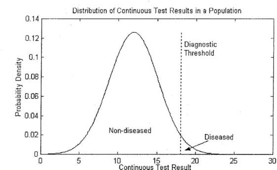
Figure 7: Single-Distribution Model. A diagnostic threshold is used to subdivide

a single distribution into diseased and non-diseased individuals. Since this

distribution represents the known population of interest, selection of the threshold also determines the prevalence of disease.

Decisions are frequently rriade in clinical medicine based on continuous

distributions where the "diseased" distribution is unknown. Serum cholesterol

and systolic blood pressure, for example, represent measurements that have

defined diagnostic offs that divide patients into two groups. Yet, these

cut-offs are not easily determined by a comparison of the distributions of these

measures between diseased and non-diseased individuals. These cut-offs are

typically determined by consensus expert opinion in relation to the distribution of

values in the "normal" population. The difficulty arises because the underlying

diseases which these measures may reflect are continuums in and of themselves.

Diagnostic decisions are also frequently made on whether a laboratory value falls

the "single-distribution paradigm." This is also the paradigm that Brenner and

Gefeller used for their investigations.

Conceptually, a more useful view of the single-distribution paradigm may

be to think of the decision threshold as dividing individuals into "low-risk" and

"high-risk" groups for an underlying disease, such as coronary artery disease,

rather than "non-diseased" and "diseased." The motivation for this view is that

although we know the distribution of values in the population as a whole,

individuals with higher values are more likely to develop disease than those with

lower values. We also know that low values do not mean the individual is

without risk.

Figure 7 illustrates the single-distribution paradigm. The known

distribution, which is typically that of healthy individuals, is subdivided into

"diseased" and "non-diseased" on the basis of a decision threshold. Unlike the

classic paradigm, the threshold is both an integral part of the definition of

"disease" and determines the prevalence of"disease" in the population in this

paradigm. The two distributions are also no longer independent. In the absence

of noise and assuming no intra-subject variability, sensitivity and specificity are

both 100%.

Since the distribution of"diseased," or "high-risk," individuals and the

distribution of"non-diseased," or "low-risk," individuals are dependent on each

other, the addition of measurement uncertainty will affect test characteristics

based on the position of the threshold. Since the threshold also determines the

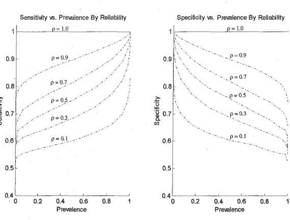
of noise. Figure 8 illustrates the affect of measurement noise on test

characteristics as a function of prevalence. This figure illustrates that even a

modest amount of noise can not only dramatically degrade the value of the test, it

does so extremely strongly as a function of prevalence. Since the reliability of the

measurement can be degraded by making measurements from an individual from

a subgroup with a different distribution, modest subgroup variation can still result

in significant degradation of test characteristics. For example, measurements of

liver enzymes are affected by BMI, age, and gender 51 Brenner and Gefeller also

show similar patterns for positive and negative predictive values and likelihood

SensitMty vs. Prevalence By Reliability Specificity \1'5. Prevalence By Reliability

= LO p= 1.0

0.9 p=0.9

~·--~--·

0.8

~

""

(f)

'· ' 0.6

0.5

0.4'----~-~-~--~-~ 0.4L--~-~--~-~-~

·0 0.2 0.4 0.6 0.8 0 0.2 0.4 0.6 0.8 1

Prevalence Prevalence

Figure 8: Variation of test characteristics in the single-distribution model versus

prevalence by varying levels of measurement reliability. There is a significant dependence of the test characteristics on "disease" prevalence in the presence of reduced measurement reliability. 1bis simulation was based on a normal

distribution with variance 4. Variance of the noise was computed as O"noU<e2 = ( O"di,tribution2- p*O"di,tribution2)/ p. Two hundred thousand samples contributed to each data point.

II.3.4 Discussion

Two paradigms exist in diagnostic testing. In the classic "two-distribution

paradigm," the characteristics of diseased and non-diseased individuals are

known. Based on this knowledge, optimal decision thresholds can be set after

taking into account the relative costs of false positives and false negatives.

Inherent in the "two-distribution paradigm" is the idea of separability. In general,

the farther apart the two distributions are the better the performance of the test.

The task in designing diagnostic instruments is to find the measure or set of

"non-diseased" distributions. A significant amount of attention has been devoted to this

paradigm, both in the design and analysis of such diagnostic systems. The ROC

curve, for example, is a construct that allows rapid assessment of the separability

of two distributions.

By contrast, the "single-distribution paradigm" makes use of a kuown

distribution and makes diagnostic decisions regarding individuals at the tails of

the distribution. Very little is kuown about the diagnostic characteristics of this

system, yet this paradigm is used on a daily basis in every medical practice.

Adverse event monitoring in clinical trials uses this paradigm as well. For

example, studies of tacrine for Alzheimer 's disease monitor alanine

aminotransferase levels in relation to multiples of the upper limits ofnormal52

Brenner and Gefeller have made a major contribution by highlighting the

problems with this system. As the simulations in the previous section show, even

small decreases in measurement reliability can have dramatic effects on test

characteristics. Since this paradigm is used on a daily basis, the implications for

health care resource use can be enormous. Simply by conceptualizing individuals

as "low-risk" or "high-risk" (for coronary artery disease, for example), there are

major implications in terms of resource use.

Perhaps the greatest flaw with the "single-distribution paradigm" is that

there is no way of telling how useful a particular measure is for diagnosing

individuals or for quantifying error rates. Since there is no second distribution

with which to compare normal and diseased individuals, measures of separability

Furthermore, withoutthe second distribution, one cannot calculate sensitivity and

specificity for a test and know how it relates to the disease of interest. Simply, the

truth about disease state is unknown and, therefore, no inferences based on

disease state can be made.

From the standpoint of subgroup variation, measurement noise does not

create spurious prevalence-dependent subgroup variation when present in the

classic "two-distribution paradigm" and it does in the "single-distribution

paradigm." However; if measurements from the two subgroups in the classic

paradigm are subject to different reliabilities, then one can have

prevalence-independent subgroup variation. Diabetics, for example, have lower variability in

cholesterol measurements than non-diabetics. 53

III

Current Approaches

A significant amount ofliterature has been devoted to the problem of

imperfect reference standards and, increasingly, to analysis of subgroup variation.

Methods for addressing the imperfect reference range from correction and

estimation procedures to methods for augmenting less than perfect references in

the hope of improving their accuracy. Since the focus of this paper is on

subgroup variation, the focus here will be on methods that use subgroup variation

to arrive at estimates of both the reference and the new test's characteristics.

Emerging methods for handling covariates affecting test characteristics are

these methods. In addition, an interesting paper addressing subgroup variation in

clinical decision making will also be discussed.

III.l

Imperfect Reference Standards

As illustrated earlier, the imperfect reference is a common problem. Even

if a perfect reference exists, it may be too expensive or invasive to be used on a

scale that would provide accurate estimates of a new test's characteristics. Since

new tests continue to be developed, and these tests need to be evaluated, methods

for addressing this problem are required. Approaches for handling this problem

have proceeded on two fronts: estimation procedures and augmentation methods

for improving the accuracy of available reference tests. A brief description of

estimation approaches and augmentation procedures will be given. This will be

followed by a consideration of the usefulness of subgroups in test parameter

estimation.

Ill.l.l Estimation Procedures

Estimation methods range from very simple algebraic methods to very

complex iterative methods. Gart and Buck in 19663 and Staquet, et al.,4 in 1981

described simple algebraic procedures for correcting reference test bias. Hui and

Walter54 published a procedure based on maximum likelihood estimation in 1980,

which served as a starting point for many of the more statistically rigorous

techniques is driven by the need to account for conditional dependence between

tests. See En0e, eta!., for a review of these methods55

Conditional independence, the property of two tests where the probability

of one test's result for a given disease state is not related the probability of the

other test's result for the same state, is difficult to satisfy in reality. If both tests

rely on blood sampling, then sampling error would affect both tests. If an

imaging test is used as a reference for another imaging test, then anatomical

features influencing diagnosis are likely to be present in both. Independence of

tests is more likely when the physical basis of the tests is very different. An

example would be the diagnosis of cancer by immunofluorescence of a tumor

specimen and the detection of a mass on cross-sectional imaging.

Early methods, such as those by Staquet, eta!., and Hui and Walter

assumed conditional independence. Unfortunately, significant biases can be

introduced when methods depending on conditional independence are used to

evaluate conditionally dependent tests. See Torrance-Rynard and Walter for an

analysis of this effect56 As a result, these simpler methods are not widely applicable.

Latent class methods represent a special case. In this approach, there is no reference test and true disease state is considered latent, or unobservable. The

results from multiple tests are used together to arrive at an estimate of the true

state via iterative maximum likelihood estimation procedures. In the case of

conditional independence, a minimum of three tests is required. Methods that

simultaneously applied tests. 57 Like other approaches, using a three-test method

that is intended for use when the tests are conditionally independent when the

tests are actually conditionally dependent will result in biased estimates. 58 Albert

and Dodd demonstrated that incorrectly specifYing the nature of the dependence

also results in biases. 57

Finally, Bayesian approaches exist for the estimation of test parameters as

well. These require selection of prior probability distributions that model already

known characteristics of tests. An overview is also given in Enoe, eta!. 55

ill.1.2 Augmentation Methods

Augmentation methods typically make use of a series of additional tests to

improve the accuracy of the imperfect reference. Two methods will be mentioned

here: discrepant analysis and composite references. Since these methods rely on

imperfect reference tests, observed test characteristics vary with prevalence.

Their use, therefore, does not eliminate the possibility of spurious subgroup

variation. Discrepant analysis was used frequently in the evaluation of

microbiological tests, but its use has since declined with recognition that this

method has inherent limitations. Composite references seek to address the

problems with discrepant analysis in a more bias neutral way.

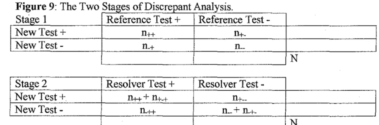
Discrepant analysis is a method for improving the estimates of a new

test's characteristics via the resolution of discrepancies58·59•60 Discrepant analysis

is a two-stage process, which is illustrated in Figure 9. In stage one, both the new

corresponding to each combination of test results is denoted nij, where i and j refer

to the test result (+ or-) for the new and reference tests, respectively. In the

second stage, individuals with discrepant results, represented by the n+. and n.+

cells, are tested again with the resolver test. The results of the resolver test trump

the result of the reference in the first stage. Therefore, a proportion of subjects

classified as false negatives in the first stage are reclassified as true negatives.

Likewise, a proportion of subjects classified as false positives are reclassified as

true positives. The effect of these two reclassifications is that the sensitivity and

specificity observed for the new test in the first stage is improved in the second

stage. This process is inherently biased.

Figure 9: The Two Stages of Discreoant Analysis.

Stage 1 Reference Test+ Reference Test

-New Test+ n++

n+-New Test- n.+ !L

N

Stage 2 Resolver Test+ Resolver

Test-New Test+ ll+++ ll+-+

ll+--New Test- ll.++ lL +

ll.+-N

The number of subJects occumng wtth each combmatwn of test 1s giVen by nijk, where i, j, and k represent the test results ( + or-) for the new, reference, and resolver tests, respectively. A third subscript is present only when the resolver is invoked. In the second stage, discrepant results are resolved by the resolver test. The resolver trumps the reference for purposes of assigning subjects with

discrepant results to a cell in the second stage.

Hadgu,61 Miller,60 and Lipman and Astles62 have described the bias

inherent in discrepant analysis when the resolver is 100% accurate. Since there is

negative, discrepant analysis falsely improves the new test's sensitivity and

specificity. Since an imperfect reference is involved, the magnitude of the bias is

dependent on prevalence.60 Thus, spurious subgroup variation is possible when

using discrepant analysis in subgroups with differing prevalences. When the

resolver is not 100% accurate biases may be larger in magnitude, but may be in

either direction. 63 When the new test and resolver test are not conditionally

independent, biases can also be significantly larger. 60

Composite reference tests address the shortcomings in discrepant analysis

in two ways. First, the reference test is a combination of tests that are chosen for

their complementary characteristics. Several highly specific tests with less than

perfect sensitivities but with differing underlying technologies, such as culture

and polymerase chain reaction (PCR), are combined such that the sensitivity of

the composite is greater than for each test alone. Second, unlike discrepant

analysis, evaluation ofthe "true" state of a subject is independent of the new test.

All subjects have the opportunity to be evaluated by all tests in the reference

independent of the result of the new test.

The execution of the composite reference can be done sequentially or all at

once. In sequential testing, tests are performed in a set order. The idea is to select

the initial tests to have perfect specificity. These tests are performed until one of

the tests is positive. Since a perfectly specific test does not make false positive

errors, the sequence can be stopped64 Alternatively, perfectly sensitive tests

could be chosen and the sequence executed until a negative test result is achieved.

PCR, for the evaluation of an enzyme immunoassay (EIA) for Chlamydia

trachomatis58 Sequential testing also has the potential to save resources by

limiting the total number of actual tests performed.

Although sequential application of the reference tests is attractive, there is

one potential problem. Delay in obtaining the additional tests in the sequence could result in interim changes in a subject's disease state. Thus, the new test and

one or more of the initial reference tests are making measurements on one disease

state while subsequent measures are measuring a different disease state.

Implementation of sequential testing procedures should ensure that all tests be

performed within a relatively small time window.

The evaluation of tests intended for screening applications is a special case

where a composite reference is required. For example, finding an abnormality on

screening mammography initiates further testing, including additional imaging

and potentially biopsy. For evaluation of negatives, it is not feasible or ethical to

subject every woman with a negative mammogram to additional studies.

Long-term follow-up is, therefore, required to adjudicate the "true" state. Another

example would be the comparison of thin-prep and liquid-based cytological

methods for cervical cancer detection. Follow-up is the only way to ascertain true

ll.1.3 Using Subgroup Variation For Test Characteristic Determination

To this point, prevalence-dependent subgroup variation due to an

imperfect reference has been presented as something to be avoided. Here,

however, the use of this type of subgroup variation to determine the

characteristics of the reference test is presented. Since imperfect reference tests

are commonly employed, it would be helpful to know what the actual

characteristics of the reference are in the populations being studied. Even

augmented references should be evaluated in this retrospective fashion to have an

idea of how much bias may be present in the data.

The use of subgroup variation to help with estimation of test

characteristics when the characteristics of the reference test are unknown was first

developed by Hui and Walter in 198054 Under the assumption that variation is

due only to differences in disease prevalence between the groups and that both the

reference test and the new test have the same, albeit unknown, characteristics in

both subgroups, they derived closed form expressions for estimates of both test's

sensitivity and specificity and the actual disease prevalences in each group. As

noted previously, a significant amount of work has been done to extend Hui and

Walter's original work However, the active use of subgroups to quantify the

effects of an imperfect reference is quite limited in the diagnostic test literature.

Two examples are Shaw et al65 and Berger et al66 in the human literature. See

En0e et al55 for additional examples from the human and veterinary medicine

In this section, Hui and Walter's closed-form estimation equations and an

alternate derivation based on Staquet et a!.' s work resulting in a somewhat

different set of equations will be presented. Simulations are presented to

understand the behavior of these equations under a variety of situations. Figure

10 shows the 2x2 contingency tables for the two subgroups and the notation used

in the formulas.

Figure 10· 2x2 Contingency Tables for 2 Subgroups with Different Prevalences

Subgroup 1 Reference Test+ Reference

Test-New Test+ a1 bl

New Test- C! dl

e1 =a1+c1 fl = bl+dl

Subgroup2 Reference Test+ Reference

Test-New Test+ a2 b2

New Test- c2 d2

ez-a2+c2 fz- b2+d2

..

SensRef, SpecRer- SensitiVIty and specifiCity of the reference SensNew, SpeCNew- Sensitivity and specificity of the new test

ID.1.3.1 The Equations of Hui and Walter

gl = a1+b1 h1 = C1+d1 N1

gz = a2+b2 h2 = Cz+d2 N2

Starting with a multinomial model, Hui and Walter derived closed form

expressions for the sensitivities and specificities of both the reference and new

test and the disease prevalences in the two subgroups via the method of maximum

Figure 11· Cell Probabilities Used in the Multinomial Model

Reference Test+ Reference

Test-New Test

+ Previ * SensNew * SensRef Previ*SensNew *(1-SensRef) + (1-Prev;)*(1-SpecN,w)*(1-SpecR,r) + (1-Prev;)*(1-SpecN~,)*SpecR,f

New Test

-

+ (1-Prev;)*SpecN,w *(1-SpecR,r) + (1-Prev;)*SpecN,w *SpecRef

P _{mu tmomra} I • . I ₌₌

n' "

;,1 ad bd

* P(Re/fesl+, NewTest-)"' P(Rejrest-,NewTest-l'

cd dd

Using the notation used by Enoe et al.,55 tbe equations they derived are:

S ensRq

=

,

2(gJN,- g/NJ

S peCR<if = (fih,-hfJINN,+d/N,-dJN,+F . , 2(gJM- g/NJ

Prev,

=

0_5 _ [(g/NJ(e/N,- eJNJ

+

+

. 2F

Prev,

=

0_5 _ [(g,/N,)(e/N,-eJNJ+(e,/N,)(g/M- g/NJ+aJM-a/M]'

2F

Where,

it is unlikely that a worthwhile reference test will have a sensitivity or specificity

less than 0.5, it should be easy to select the appropriate solution. Prior knowledge

about the test should also be helpful in selecting the appropriate solution. Another

difficulty is that division by zero is encountered in the test parameter formulas

when the new test's parameters (SensNew and SpeCNew) are being calculated and

the measured prevalences as determined by the reference test are equal between

the two subgroups and vice versa. In situations were there is insufficient prior

information to help select the appropriate solution or one is near a singularity,

iterative methods will be required.

III.1.3.2 Direct Algebraic Approach

III.1.3.2.1Reference Test Characteristics Known

Figure 12: 2x2 Contingency Matrix Showing Cell Count Corrections For Imperfect Gold Standard With Known Characteristics

Reference Test+ Reference

Test-New Test+ (a-b*(l/SpecRe~·-1))/SensR,f (b- a*(l/SensRer- 1))/SpecRef

New Test- (c- d*(l/SpecRer- 1))/SensRef (d- c*(1/SensR,r-1))/SpeCRef

As preamble to the derivation for the case with unknown reference test

characteristics, formulas for the estimates of the new test's characteristics when

the reference test characteristics are known are given here. Both Staquet et a!. 4

and Gart and Buck3 provide algebraic methods for correcting observed test results

shows the corrections for known reference test characteristics to the observed cell

counts. Formulas for sensitivity, specificity, and prevalence follow from these

corrections:

S enSNew = (a+b)*Spec&J-b ,

N* SpeC&J-(b+d)

S ~eCNew

=

,

N* SenSReJ-(a +c)

Prev= N*(SpecR<J-l)+(a+c). N

*

+

With these equations, special cases can be considered. First, we note that

the correction for sensitivity is dependent only on the specificity of the reference

and the correction for specificity is dependent only on the sensitivity of the

reference. Thus, in the event that the reference test is known to have 100%

specificity, the observed sensitivity is no longer biased:

a

SensNew

=

Similarly, if the reference test is known to have 100% sensitivity, then the

observed specificity is no longer biased:

d

SpeCNew

= - - ,

Ifboth tests have 100% specificity, then the sensitivities of the two tests are:

a a

SensNew

=

=