Application of Particle Swarm Optimization
to Optimal Design of Cascade Stilling Basins
M. Daraeikhah
1, S.H. Meraji
1and M.H. Afshar
1;Abstract. This paper employs the Particle Swarm Optimization (PSO) method to solve the problem of the optimal design of cascade stilling basins. PSO is a relatively recent heuristic search method whose mechanism is inspired by the swarming or collaborative behavior of biological populations. The objective of this research is to minimize the total construction cost of cascade stilling basins, which is a function of height of the falls and length of stilling basins, while fullling the hydraulic and topographical criteria. To illustrate the application of PSO, a benchmark design is taken from the work of Vittal and Porey [1] on a cascade stilling basin for the Tehri Dam, India.
Keywords: Particle swarm optimization; Cascade stilling basins; Global optimization.
INTRODUCTION
Energy dissipation below hydraulic structures, like dams, barrages across rivers and control weirs on canals, is accomplished conventionally by single-fall hydraulic jump-type stilling basins and roller buckets on trajectory buckets. However, in the case of high head dams, the kinetic energy at the toe of the spillways is very high and the tailwater depths available in the river are often inadequate for the former two devices. Narrow and curved gorges, consisting of fractured rock, prohibit the adoption of the last. In such situations, especially for earth and rock ll dams, a system of falls cascading down the side of a valley, with a stilling basin below each fall, can be used as an alternative spillway. The rst design method for this system was developed by Vittal and Porey [1]. In this method, the height of the lowest fall is determined by the available river tailwater depth at design discharge, whereas the number of preceding equal-height falls are determined by the available distance for the spillway sections and stilling basins. Thus, it seems to be empirical to some extent and does not lead to an optimal design, so, it is necessary to use an alternative approach to obtain an optimal solution. In this paper, a PSO algorithm is proposed for the optimal design of cascade
1. Department of Civil Engineering, Iran University of Science and Technology, P.O. Box 16765-163, Tehran, Iran. *. Corresponding author. E-mail: [email protected] Received 27 August 2006; received in revised form 8 August 2007; accepted 5 February 2008
stilling basins. The results of the PSO model are compared with the results generated from the Vittal and Porey method. It is also shown that the PSO approach can produce better designs than those of the Vittal and Porey method, in almost all the cases considered. This paper is organized in ve major sections. First, the PSO algorithm is summarized. Second, the Vittal and Porey method is explained. Next, an optimization model of cascade stilling basins, using the PSO algorithm, is introduced, and a case study and conclusions are presented in the last two sections.
PARTICLE SWARM OPTIMIZATION
In 1995, Russell Eberhart and James Kennedy [2] applied a model to the problem of nding optima in a search space, which can be compared to a ock of birds looking for a food source, and created the PSO algorithm. The literature describing the application of PSO to water engineering is not abundant. Gill et al. [3] described a multi-objective optimization ap-proach using PSO for parameter estimation in hydrol-ogy.
Suribabu [4] applied a PSO for deriving operation policies for maximum hydropower generation. Also, in 2006, Suribabu and Neelakantan [5] used PSO to the optimal design of water distribution networks. Finally, Meraji and Afshar [6] used the algorithm to the reservoir operation of the Dez Dam in Iran. Also, they combined the PSO optimizer with an SWMM simulator
to develop a model for the optimal design of a ood control system.
In PSO, a collection of particles, called a \swarm", move around in search space looking for the best solution to an optimization problem. All particles have their own velocity that drives the direction they move in. This velocity is aected by both the position of the particle with the best tness and each particle's own best tness. Fitness refers to how well a particle performs. In a ock of birds, this might be how close a bird is to a food source; in an optimization algo-rithm, tness is a function of the objective function. Each particle's location is given by the parameters of the given optimization problem and a particle moves around in search space by adapting and changing these parameter values. At each time step, the particle's tness is measured by observing the parameter values (location) of the particle. A particle keeps track of the best position it has reached so far (called the personal best position) and is also aware of the position of the overall best particle at a certain time step (called the globally best position). At each time step, the particle tries to adapt its velocity (i.e. speed and direction) to move closer to both the globally best position and the personal best position, in order to try and improve its tness. Two variants of the PSO algorithm were developed; one with a global neighborhood and one with a local neighborhood. According to the global variant, each particle moves towards its best previous position and towards the best particle in the whole swarm. On the other hand, according to the local variant, each particle moves towards its best previous position and towards the best particle in its restricted neighborhood [2]. In the following paragraphs, the global variant is exposed (the local variant can be easily derived through minor changes).
Suppose that the search space is D-dimensional, then, the ith particle of the swarm can be represented by a D-dimensional vector, Xi = (xi1; xi2; ; xiD)T.
The velocity (position change) of this particle can be represented by another D-dimensional vector, Vi = (vi1; vi2; ; viD)T. The best previously
vis-ited position of the ith particle is denoted as Pi =
(pi1; pi2; ; piD)T. Dene g as the index of the best
particle in the swarm (i.e., the gth particle is the best) and let the superscripts denote the iteration number, then, the swarm is manipulated according to the following two equations [2]:
vn+1
id =vidn+crn1;i;d(pnid xidn)+crn2;i;d(pngd xnid); (1)
xn+1
id = xnid+ vn+1id ; (2)
where d = 1; 2; ; D; i = 1; 2; ; N, and N is the size of the swarm; c is a positive constant, called the acceleration constant; r1;i:d, r2;i;dare random numbers,
uniformly distributed in [0; 1]; and n = 1; 2; deter-mines the iteration number.
Equations 1 and 2 dene the initial version of the PSO algorithm. Since there is no actual mechanism for controlling the velocity of a particle, it was necessary to impose a maximum value, Vd;max, on it (i.e. Vd;max
Vidn+1 Vd;max). If the velocity exceeded this
thresh-old, it was set equal to Vd;max. This parameter proved
to be crucial, because large values could result in particles moving past good solutions, while small values could result in insucient exploration of the search space. The value of Vd;max is usually chosen to be
K Xd;max with 0:1 k 1:0, where Xd;max is the
upper bound of the search space of particles in the dth dimension [7]. This lack of a control mechanism for the velocity resulted in low eciency for PSO, compared to EC techniques [8]. Specically, PSO located the area of the optimum faster than evolutionary computation techniques, but once in the region of the optimum, it could not adjust its velocity step size to continue the search at a ner grain. The aforementioned problem was addressed by incorporating a weight parameter for the previous velocity of the particle. Thus, in the latest versions of the PSO, Equations 1 and 2 are changed to the following ones [9,10]:
vn+1
id = (wvidn + c1rn1;i;d(pnid xnid)
+ c2r2;i;dn (pngd xnid)); (3)
xn+1
id = xnid+ vn+1id ; (4)
where w is called inertia weight; c1and c2are two
pos-itive constants, called cognpos-itive and social parameter, respectively; and is a constriction factor, which is used alternatively to w and to limit velocity. The role of these parameters is discussed in the next section. The Parameters of PSO
The role of the inertia weight, w, in Equation 3, is considered critical for the PSO's convergence behavior. The inertia weight is employed to control the impact of the previous history of velocities on the current one. Accordingly, the parameter, w, regulates the trade-o between the global and local exploration abilities of the swarm. A large inertia weight facilitates global exploration (searching new areas), while a small one tends to facilitate local exploration, i.e. ne-tuning the current search area. A suitable value for the inertia weight, w, usually provides a balance between global and local exploration abilities and, consequently, re-sults in a reduction of the number of iterations required to locate the optimum solution. Initially, the inertia weight was constant. However, experimental results indicated that it is better to initially set the inertia to
a large value, in order to promote global exploration of the search space, and gradually decrease it to get more rened solutions. Thus, Shi and Eberhart [9,10] made a signicant improvement in the performance of the PSO, with a linearly varying inertia weight over the iterations, which linearly varies from wmax at the
beginning of the search to wmin at the end. Thus,
the following weighting function is usually utilized in Equation 3:
w = wmax (wmaxiterwmin) n
max ; (5)
where wmax and wminare the maximum and minimum
value of inertia weight, respectively, n is the current iteration number and itermaxis the maximum iteration
number. The parameters c1, c2 in Equation 3 are not
critical for PSO's convergence. However, proper ne-tuning may result in faster convergence and alleviation of local minima. An extended study of the acceleration parameter in the rst version of PSO is given in [11]. As default values, c1 = c2 = 2 were proposed, but
experimental results indicate that c1= c2= 0:5 might
provide even better results. Recent work reports that it might be even better to choose a larger cognitive parameter, c1, than a social parameter, c2, but with
c1+ c2 4 [12]. The parameters r1 and r2 are used
to maintain the diversity of the population and they are uniformly distributed in the range [0, 1]. The constriction factor, , controls the magnitude of the velocities, in a way similar to the Vd;max parameter,
resulting in a variant of PSO dierent from the one with the inertia weight.
VITTAL & POREY DESIGN PROCEDURE The design of cascade stilling basins was rst in-troduced by Vittal and Porey in 1987 [1]. In the following paragraphs, the considerations and procedure for the design of cascade stilling basins, as well as the necessary relationships for design, are presented. The procedure for the design of cascade stilling basins can be summarized as:
1. Determination of the height and the length of the terminal fall and the proportioning of a suitable stilling basin for it;
2. Determination of the number and nature of the preceding falls;
3. Determination of the height of the raised crest for the preceding falls.
Terminal Fall
The height of terminal fall Ht (the dierence in the
levels of the terminal crest and river bed in Figure 1)
Figure 1. Longitudinal section of cascade of falls.
is determined, such that the post jump depth of ow for hydraulic jump formation at the design discharge is equal to the tailwater depth available in the river. This will avoid deep excavation of the river bed, which would be expensive and might induce dangerous landsliding of the valley slope.
Ht= gy 4 td
7:80q2
d; (6)
where qd is the unit design discharge, ytd is the
tailwater depth at the design discharge and g is the acceleration due to gravity. The deciency or excess of tailwater at partial discharge can be known by comparing the Free-Jump-Height Curve (FJHC) for the terminal fall with the Tailwater Rating Curve (TWRC) of the river. In the event of a tailwater excess, the stilling basins need not be depressed, whereas, in the event of a deciency, the oor will be lowered by zt, equal to the maximum dierence in the ordinates
of FJHC and TWRC at partial discharge. With the drop in the oor level, the height of the terminal crest above the stilling basin oor, Pt, will now be
replaced by Ht+ zt. The length of the stilling basin
for the terminal fall will vary according to the Froud number [13]:
Lt=
(
4:25y2d Fr1 4:5
2:80y2d Fr1< 4:5 (7)
where Ltis the length of the stilling basin for terminal
fall, y2d is the post jump depth of ow at the design
discharge and the Froude number is the pre jump Froude number for the last cascade, which may be computed from Equation 8 by trial and error [13]:
g1 2P
3 2
t
q =
1 2Fr
4 3
1 + Fr
2 3
1 211
3C23
3 2
; (8)
Preceding Falls
The length required to accommodate all the spillway section and stilling basins, (L), is:
L = (N 1)(xp+ Lp) + (xt+ Lt); (9)
in which xtand xp are the base widths of the spillway
sections; Ltand Lpare the lengths of the stilling basins
for the terminal fall and preceding falls, respectively; and N is the number of cascades. Adopting the ogee prole given by [13], one obtains the following:
y
h0d = 0:50
x h0d
1:85
; (10)
in which x and y are the coordinates of the spillway prole and h0dis the total head over crest at the design
discharge. The following equations can be written for xtand xp:
xt= 1:455h0d
Pt
h0d
1
1:85
; (11)
xp = 1:455h0d
P h0d
1
1:85
: (12)
The equation suggested by Poggi [14] for the oor length of stilling basins without appurtenance can be adopted for a cascade system:
Lp= 6(y2 y1); (13)
where y1and y2are the pre-jump and post-jump depths
of ow, respectively.
The height of the crest above the stilling basin oor, (P ), for the preceding falls of equal height can be calculated from Equation 14 [1]. Assuming a known value of N, Equation 14 can be solved for P by trial and error:
P = H0NHt+ 1:671q
1 2
dP
1 4
g1 4
qd
Cp2g 2
3
+ 0:179 qd g1
2P12: (14)
To force the jump, a control or crest, preferably of ogee prole, is placed at the end of the oor. The required height of crest z for jump formation at the design discharge is given by:
z = P HN0 H1t: (15)
Here, P is computed from Equation 14, H0 is the total
fall and Htis the height of the terminal fall.
OPTIMAL DESIGN OF CASCADE STILLING BASINS
The aim of the PSO model is to minimize the con-struction cost of the system by changing the design variables, i.e. height of falls and length of stilling basins, while fullling the topographical and hydraulic criteria. The design principles used in the optimization model are those of the Vittal and Porey method, with the dierence that, in the Vittal and Porey method, the length and the height of the preceding falls are equal, thus, it is not necessarily optimal. However, the PSO model can choose dierent values for the height and length of the falls in order to design a system with optimum cost. The optimization model can be mathematically stated as follows:
Minimize f =XN
i=1
(f1(Pi; `i) + f2(Pi; `i)); (16)
where f is the total cost of construction, which is a function of the design variables, and f1 and f2 are
the concrete and excavation costs of the ith cascade, respectively, Pi is the height of the ith fall, li is the
length of the ith fall, and N is the total number of cascades. The general constraints of the system are topographical and hydraulic as explained in the following paragraphs.
Topographical Constraints
N
X
i=1
(L(i) + x(i)) = La; (17)
H0 N
X
i=1
(Pi z(i)) zt= 0; (18)
where La is the total length available, which is the
horizontal distance between the center point of the rst fall and the terminal point of the last basin; zt is
equal to the maximum dierence in the ordinates of FJHC and TWRC at partial discharge; and z(i) is the height of the crest for the ith fall. The required height of crest z(i) for jump formation at the ith fall and the design discharge is dened as follows [1]:
z(i) = 1:671qd0:5Pi
g1 4
qd
Cp2g 2
3
+ 0:179 qd g1
2P 1 2
i
;
z(N) = 0; (19)
where C is the discharge coecient, qd is the unit
Hydraulic Constraints
Maximum and Minimum Height of the Fall
Pmin Pi Pmax: (20)
Pmax and Pmin are the maximum and minimum
allow-able heights of the falls, respectively, which have been calculated using the maximum and minimum pre-jump Froude numbers of the ow in the corresponding stilling basins. For the range of Froud numbers of the incoming ow between 4.5 and 9, a stable and well-balanced jump occurs. Turbulence is conned to the main body of the jump and the water surface downstream is comparatively smooth [13]. Thus, Fr1;max = 9 and
Fr1;min= 4:5:
Pmax= q
2 3
d
g13
1 2Fr
4 3
1 max+ Fr
2 3
1max
1 213C23
; (21)
Pmin= q
2 3
d
g1 3
1 2Fr
4 3
1min+ Fr 2 3
1min
1 21
3C23
: (22)
Minimum Length of Stilling Basins
li li;min; (23)
where li;minis the minimum allowable length of the falls
and is determined based on the so-called throw length of the jet and the necessary length of a hydraulic jump.
li;min= 6(y2;i y1;i): (24)
with: h0D=
qd
Cp2g 2
3
; (25)
y1;i=
qd
g1 2Fr1i
2 3
; (26)
y2;i=y21;i
q
1 + 8Fr2
1i 1
: (27)
y1;iand y2;iare the pre-jump and post-jump depths of
ow, respectively; Fr1;iis the pre-jump Froude number
in the ith fall; and C is the discharge coecient. Minimum Height of Terminal Crest Above Stilling Basins Floor
P (N) Ht+ zt: (28)
The basin must be made deep enough to provide for the full post-jump depth of ow (or some greater depth, to
include a factor of safety) at maximum spillway design discharge. A tailwater depth greater than the required post-jump depth is conducive to the formation of a so-called drowned jump (with the drowned jump, instead of achieving a good-type dissipation by intermingling of the upstream and downstream ows, the incoming jet plunges to the bottom and carries along the entire length of the basin oor at high velocity). The above constraint assures that the required post-jump depth will be always greater than the tailwater depth.
The problem's constraints now can be written in standard form as:
g1= H0 N
X
i=1
(Pi z(i)) zt= 0; (29)
g2= La N
X
i=1
(L(i) + x(i)) = 0; (30)
g3= 1 PPi
max 0; (31)
g4= 1 PPi
min 0; (32)
g5= 1 l li
i min 0; (33)
g6= 1 HtP (N)+ zt 0: (34)
CASE STUDY
In this section, both the Vittal and Porey method and the proposed PSO model are used for the design of the Tehri dam spillway and the results are compared. The Tehri dam is an earth and rockll dam, 260.50 m high, on the river Bhagirathi, a tributary of the river Ganga valley of the central Himalayan region of India. The spillway is located on the right abutment of the dam. At the dam site, the exposed rocks are alternate bands of weak quartzites and phyllites. Various alternatives for the type of spillway were considered. A single-stage hydraulic jump-type stilling basin involves a velocity of 66.00 m/s in the basin and a 15.00 m riverbed excavation to make up for the deciency of tailwater depth. A chute spillway, followed by a ski-jump bucket, throws trajectories on the hill slopes of the narrow valley, and the rocks cannot withstand signicant impact. Further, the situation of the hills, due to the spray, may result in sheet landslides. Thus, a spillway with a cascade of falls and stilling basins will be adopted. A 95.00 m wide control structure, consisting of ve bays of 16.00 m each, separated by 3.75 m thick piers, is provided with a full-reservoir level of 818.00 m. Other design data are listed in Table 1.
Table 1. Design data for Tehri dam.
Characteristic Datum Design discharge, Qd 11000.00 m3/s
Total fall, H0 218.00 m
River level at exit 600.00 m Length of spillway crest at lower falls 95.00 m Tailwater depth at design discharge, ytd 29.20 m
Distance available between rst crest and exit, La 778 m
Figure 2. TWRC and FJHC for terminal fall - Tehri dam spillway.
As seen in Figure 2, the TWRC is entirely below the FJHC at partial discharge, and the maximum tailwater deciency of 2.06 m occurs at 1960 m3/s.
Hence, zt= 2:06 m.
Considering the site condition and its type, there exist just two types, N = 3 and N = 4, in the feasible space. In the following, the results of the design by the Vittal and Porey and PSO methods are compared (all dimensions in meters). It is notable that, in this study, the concrete and excavation costs per cubic meter are considered to be 180000 and 23100, respectively.
PSO has several explicit parameters, whose values can be adjusted to produce variations in the way the algorithm searches the solution space. Shi and Eber-hart [9,10] tried to examine the parameter selection of these parameters. According to their examination, the
following parameters are appropriate and adopted in this paper:
Wmax= 0:9; Wmin= 0:4; c1= c2= 2:0:
In the following, the results are presented.
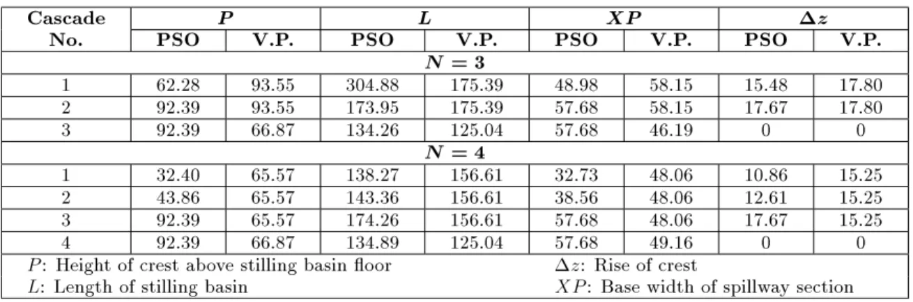
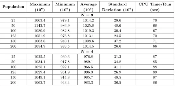
Table 2 compares the results obtained by the proposed PSO algorithm with that of Vittal and Porey. Table 3 shows the maximum, minimum, average and standard deviations of the solution costs obtained in 10 runs on a Pentium 4 with a CPU of 2.40 GHz and 512 MB of RAM. As mentioned above, for each swarm size, the model has been run ten times and the best solution is selected as an optimal cost, as presented in Table 4. As can be seen from Table 4, in both cases the PSO has produced superior results to the Vittal and Porey method. The savings oered by the PSO are about 22 and 17 percent for the number of cascades equal to 3 and 4, respectively. Figures 3 and 4 schematically compare the PSO and Vittal and Porey solutions for N = 3 and N = 4, respectively. As can be seen clearly in both cases, PSO has chosen a smaller height for the rst cascade than that of Vittal and Porey.
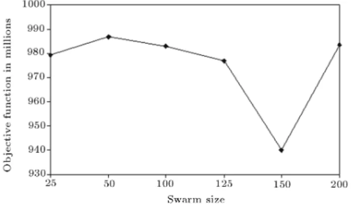
There is no rule as to how many particles should be used to solve a specic problem. A large number of particles allow the algorithm to explore the search space faster; however, the tness function needs to be evaluated for each particle, so the number of particles will have a huge impact on the speed at which the simulation will run. Here, a sensitivity analysis is carried out on the swarm size for a xed number of
Table 2. Comparisons of the results obtained by PSO and vittal and porey method.
Cascade P L XP z
No. PSO V.P. PSO V.P. PSO V.P. PSO V.P. N = 3
1 62.28 93.55 304.88 175.39 48.98 58.15 15.48 17.80 2 92.39 93.55 173.95 175.39 57.68 58.15 17.67 17.80 3 92.39 66.87 134.26 125.04 57.68 46.19 0 0
N = 4
1 32.40 65.57 138.27 156.61 32.73 48.06 10.86 15.25 2 43.86 65.57 143.36 156.61 38.56 48.06 12.61 15.25 3 92.39 65.57 174.26 156.61 57.68 48.06 17.67 15.25 4 92.39 66.87 134.89 125.04 57.68 49.16 0 0 P : Height of crest above stilling basin oor z: Rise of crest
Table 3. Solution costs and average run time obtained in 10 runs. Population Maximum
(106)
Minimum (106)
Average (106)
Standard Deviation (106)
CPU Time/Run (sec) N = 3
25 1063.4 979.1 1014.2 28.6 70 50 1143.7 986.9 1025.8 48.6 68 100 1080.9 982.8 1019.3 30.4 67 125 1051.9 976.8 1013.1 24.5 70 150 1063.6 940.1 1008.6 37.2 71 200 1054.9 983.5 1014.5 26.6 66
N = 4
25 1025.5 930.3 976.8 31.3 87 50 1034.1 917.8 989.1 34.8 85 100 1025.1 922.1 966.5 31.1 88 125 1029.4 951.9 996.3 26.9 89 150 1049.1 914.8 985.7 48.5 87 200 1063.7 943.4 983.3 36.5 86
Figure 3. Comparison between PSO and Vittal and Porey designs (N = 4).
Figure 4. Comparison between PSO and Vittal and Porey designs (N = 4).
50,000 function evaluations. Figures 5 and 6 show the variations of the solution costs with the swarm sizes used for N = 3 and N = 4, respectively. It is seen that the best results are obtained with swarm sizes of 150 for the number of cascades equal to 3 and 4. Figures 7 and 8 show the convergence characteristics
Table 4. Optimal unit cost of the designs (106).
N PSO V.P. 3 940 1194 4 914 1094
of the PSO for N = 3 and N = 4. It is clearly seen that the method has been eectively able to locate the best solutions within 20,000 function evaluations, long before the maximum number of function evaluations has been exhausted.
CONCLUSION
A Particle Swarm Optimization (PSO) algorithm is applied to the cascade stilling basins problem. A cascade system of falls with a stilling basin below each fall is well suited to energy dissipation below high head spillways. The previous design method of a cascade stilling basin was based on the hypothesis that the length and height of the preceding falls are equal; thus, it seems to be empirical, to some extent, and not necessarily optimal. While a lot of meta-heuristic algorithms have been developed for combi-natorial optimization problems, PSO has been basi-cally developed for continuous optimization problems. One particularly interesting aspect of the algorithm is that there are very few parameters to adjust. Also, PSO comprises a very simple concept and can be implemented in a few lines of computer code. It requires only primitive mathematical operators and is computationally inexpensive, in terms of both memory requirements and speed. The performance of PSO is compared to that of the Vittal and Porey method on a test example of the Tehri dam spillway. The result indicated that the optimization model is capable of signicant savings in the cost of cascade stilling basins.
Figure 5. Sensitivity of PSO to swarm size (N = 3).
Figure 6. Sensitivity of PSO to swarm size (N = 4).
Figure 7. PSO convergence curve (N = 3).
Figure 8. PSO convergence curve (N = 4).
REFERENCES
1. Vittal, N. and Porey, P.D. \Design of cascade stilling basins for high dam spillways", ASCE, Journal of Hydraulic Division, ASCE, 113(9), pp. 225-237 (1987). 2. Eberhart, R. and Kennedy, J. \A new optimizer using particle swarm theory", Proceedings of the Sixth In-ternational Symposium on Micro Machine and Human Science, Nagoya, Japan, pp. 39-43, Piscataway, NJ: IEEE Service Center (1995).
3. Gill, M.K., Kaheil, Y.H., Khalil, A. and Kee, M.M. \Multiobjective particle swarm optimization for pa-rameter estimation in hydrology", Water Resources Research, 42(7), W07417 (2006).
4. Suribabu, C.R. \Particle swarm optimization tech-niques for deriving operation policies for maximum hydropower generation: A case study", International Journal of Ecology and Development, 4(W06), pp. 66-85 (2006).
5. Suribabu, C.R. and Neelakantan, T.R. \Design of water distribution networks using particle swarm op-timization", Urban Water Journal, Taylor and Francis Publishing, 2(3), pp. 1-10 (2006).
6. Meraji, S.H., Afshar, M.H. and Afshar, A. \Reservoir operation by particle swarm optimization algorithm", 7th International Conference of Civil Engineering, Tehran, Iran (2006).
7. Eberhart, R., Simpson, P. and Dobbins, R., Computa-tional Intelligence PC Tools, Boston: Academic Press Professional, p. 491 (1996).
8. Angeline, P.J. \Evolutionary optimization versus par-ticle swarm optimization", in Evolutionary Program-ming VII, V.W. Porto, N. Saravanan, D. Waagen and A.E. Eiben, Eds., Springer, pp. 601-610 (1998). 9. Shi, Y. and Eberhart, R. \Parameter selection in
par-ticle swarm optimization", Proc. of the 1998 Annual Conference on Evolutionary Programming, San Diego, pp. 591-600 (1998a).
10. Shi, Y. and Eberhart, R.C. \A modied particle swarm optimizer", Proc. of IEEE International Conference on Evolutionary Computation (ICEC'98), Anchorage, Alaska, May 4-9, pp. 69-73 (1998b).
11. Kennedy, J. \The behavior of particles", in Evolution-ary Programming VII, V.W. Porto, N. Saravanan, D. Waagen and A.E. Eiben, Eds., Springer, pp. 581-590 (1998).
12. Carlisle, A. and Dozier, G. \An o-the-shelf PSO", Proceedings of the Particle Swarm Optimization Work-shop, pp. 1-6 (2001).
13. U.S. Bureau of Reclamation \Hydraulic design of still-ing basins and bucket energy dissipaters", Engineerstill-ing Monograph No. 25, U.S. Dep. of Interior, Bureau of Reclamation, Denver (1985).
14. Poggi, B. \Lo scaricatori a scala di stramazzi: Criteri di calcolo rilievei sperimentali", L'Energia Elettrica, 33(1), pp. 33-40 (1956).