Sharif University of Technology
Scientia IranicaTransactions A: Civil Engineering www.scientiairanica.com
Eects of edge rate of the designed line markings on
the following time headway
N. Ding
a, S. Zhu
a;, H. Wang
aand N. Jiao
ba. School of Transportation, Wuhan University of Technology, 1178 Heping Avenue, Wuhan, Hubei 430063, China.
b. Planning Research Studio, Department of Transportation of Hubei Province, 428 Jianshe Avenue, Wuhan, Hubei 430030 China. Received 17 June 2015; received in revised form 18 February 2016; accepted 8 July 2017
KEYWORDS Edge rate; Line marking; Car-following; Time headway; Distance perception; Speed perception.
Abstract. Time headway is an important indicator for evaluating car-following safety. To study the inuence of edge rate on time headway in car-following, three patterns of line marking were designed and placed on a real-world expressway, with actual vehicle ow data collected. Statistical analyses showed that (1) Time headways raised after the installation of line markings compared with the original situation; and (2) When the value of edge rate fell in [5 Hz,14 Hz], the time headway rose along the increase in the edge rate. Furthermore, the increases in time headways were interpreted in relation with the leveling up of the drivers' risk perception due to its overestimation in speed and underestimation in distance caused by edge rate. The nding of this study suggests that the designed line markings may benet engineers and decision makers in providing them with a new approach to cope with critical issues in trac safety.
© 2017 Sharif University of Technology. All rights reserved.
1. Introduction
Rear-end collisions are the most common accident type (accounted for 40.4%) among all collision accidents, which have led to thousands of casualties in China in 2010 [1]. Thus, it is urgent to cope with this issue with eective methods to level up roadway safety.
For a long time, headway (both time headway and distance headway) has been used as an important indicator for evaluating car-following safety [2-7]. Time headway is the time interval between two vehicles. It is distance headway, bumper to bumper distance between two consecutive vehicles in a lane, divided by the speed of the following vehicle. Generally, car-following models are built to obtain the distribution
*. Corresponding author. Tel.: +8613995680983; Fax: +8613995680983
E-mail addresses: andrei8901@gmail.com (N. Ding); zhusy2001@163.com (S. Zhu); wanghong2004317@sina.com (H. Wang); 421946755@qq.com (N. Jiao)
and evaluation of time headway [8-11]. Thus, it can easily be seen that the drivers' judgments of speed and distance are the main factors in the control of time headway.
It was reported that 90% of the information that drivers used to make a decision/judgment came from visual information [12]. Boer [13] argued that in each driving task, drivers utilized a set of highly informative perceptual variables to guide decision making and con-trol (perceptual rather than Newtonian input). Simi-larly, Andersen and Sauer [14] dened car-following as a perceptual process which could be determined by the visual angle. Also, Van Winsum [15] commented on the car-following study of Brackstone and McDonalds [8] that human factors like fatigue, visual conditions, and mental eort and attention could aect driver's control of time headway. It can be reached from the above research that visual information plays an important role in the drivers' judgments and/or perceptions of speed and distance.
vari-ables that have been used in speed control, which is dened as the rate at which local discontinuities cross a xed reference point in the observer's eld of view [16]. According to Shen et al. [17,18], edge rate can also be derived from the temporal frequency (ft) and the
spatial frequency (fs). Signals can be measured by
temporal frequency (ft) when they vary periodically
in time, which normally can be measured by a unit of Hz. Correspondingly, signals can also be measured by spatial frequency (fs) when they vary periodically in
space (typically in depth). Edge rate equals temporal frequency, derived from relative motion, when the spatial frequency is constant.
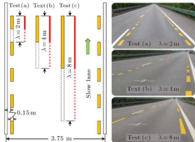
According to the denition of ER, the edge rate that a person can perceive is aected by both the density of line markings and the self-speed. Density reects the spatial frequency of the line markings and self-speed is the derivation of the temporal frequency or edge rate. It means that even when the drivers are exposed to the same line markings, the strength of edge rate they perceive would be dierent if they are driving at dierent speeds. Thus, for the purpose of distinguishing the eects of spatial frequency and edge rate, here, we dene the unit of line marking as the sum of one single marking length and its adjacent interval, which is denoted by lambda (). Figure 1 depicts an introductory picture to explain these important terms appearing in this paper.
In further research, Francois et al. [19] predicted that edge rate, produced by textures on the ground surface, could result in drivers' overestimation of self-speed and, in turn, lead to reduction in actual self-speed. In addition, speed reduction caused by the edge rate can also be found in high-speed motion. Larish and Flach [20] reported that the estimated speed rose with the increase of edge rate. Rakha et al. [21] designed a form of transverse bars with a constant gap, and the eld data showed a 6 km/h reduction in the mean speed and an 8 km/h reduction in the 85th percentile speed. Furthermore, based on eld observations, Liu et al. [22] found that drivers perceived the greatest speed overestimation when the value of edge rate varied from
Figure 1. An introductory sketch map of important terms.
8 Hz to 16 Hz, which accordingly led to the greatest reduction in actual speed. Nevertheless, the previous research mainly focused on the eects of speed changes of the leading vehicle on time headway of the following vehicle, which more or less neglected that there could be speed changes both in the leading and the following vehicle when they were both exposed to line markings. Hence, this study is to examine the relation between edge rate and time headway, considering the eects of edge rate on both the leading vehicles and the following vehicles.
On the other hand, the perception of distance is also aected by visual information. Gibson [23] proposed the \Ground Theory", which predicted that when the common ground surface was disrupted, the visual system was unable to establish a reliable refer-ence frame and consequently failed to obtain correct absolute distance. By utilizing the methods of \blind-folded walking task" and \perceptual matching task", Sinai et al. [24] reported distance underestimation occurred in the condition of texture discontinuities, which to a certain extent veried the prediction of Gibson. Similarly, Wu et al. [25] and Yarbrough et al. [26] presented discontinuous textures on the ground in virtual reality environment, and found that the distance was underestimated by observers. Specically, Feria et al. [27] referred to this distance underestimation phenomenon as the \discontinuity ef-fect". Conclusively, these experiments about distance perception were primarily conducted in static virtual reality scenes, which were quite dierent from high-speed motion in real environments. In addition, only simple textures were demonstrated in their studies (i.e., grass versus cement in Sinai et al.'s [24] and spaced stripes in Wu et al.'s [25], Yarbrough et al.'s [26], and Feria et al.'s [27]). Besides, the span of the textured area and the distance were supposed to be judged relatively limited (12.29 m in Feria's, and 7.62 m in Sinai's). To some extent, the designed line markings, as depicted in Figure 1, may contain discontinuous visual information. Hence, it is necessary to examine if there is a similar eect of distance underestimation caused by this kind of line markings.
In brief, previous studies on time headway pri-marily focused on the speed of the leading vehicle, but neglected the eect of self-speed or rather the state of speed reduction in car-following. The studies on distance perception were still with some limitations to develop the \discontinuity eect" into the real world of high-speed motion. Hence, in this study, we com-bine the thoughts of the perception of speed and the perception of distance to study their inuences on time headway in car-following. Given these considerations, we propose the following two hypotheses:
headway since they cause speed reduction due to speed overestimation in drivers;
2. Designed line markings can lead to distance under-estimation in high-speed driving situation.
To verify these hypotheses, we conducted a series of eld experiments in a real-world expressway in China.
2. Experiment 2.1. Overview
A yellow pre-formed adhesive tape was established aside the two original white markings of the slow lane of a road to exhibit the designed line markings. Vehicle ow data, like speed and time headway, were collected via video cameras set at consecutive observa-tion secobserva-tions. The mean speeds and time headways of observation sections before and after the installation of line markings were compared.
2.2. Experimental site
The segment of Shanghai and Chongqing Expressway (coded G50) at Yichang, Hubei Province, P.R. China, was chosen as the experimental site. It was a two-way-four-lane expressway with a design speed of 80 km/h and a land width of 3.75 m. The Annual Average Daily Trac (AADT) was 11,134 vehicles per day. The exact location of this experimental site was between 1220.2 km to 1221.1 km of G50, at which it was a at and straight segment. Along the direction of mileage increment, this straight segment was connected with a right-turn curve in upstream and with another series of curves in downstream. Note that there was no tunnel or overpass within the 300 m area, nor any exposed surveillance system for violations capture.
2.3. Design of line markings
A 300-m-length slow lane was installed with line mark-ings (see Figure 2). As the speed varied from 50 km/h to 100 km/h, three units of line markings, i.e. test (a) ( = 2 m), test (b) ( = 4 m), and test (c) ( = 8 m), were chosen to cover the scope of spatial frequency and edge rate. Given the reciprocal relationship between lambda and spatial frequency shown in Figure 1, we could get an equation regarding spatial frequency, that is:
test (a) = 2 test (b) = 4 test (c):
Within the speed range, the corresponding values of edge rate fell in 6.9 Hz-13.9 Hz in test (a), 3.5 Hz-6.9 Hz in test (b), and 1.7 Hz-3.5 Hz in test (c). Figure 2 shows the design of line markings and the real scene on the slow lane.
2.4. Data collection and treatments
Six NC200 trac analyzers were sequentially
posi-Figure 2. Design of line markings.
tioned in the center of the slow lane, to collect data like speed, time headway, and vehicle type at each ob-servation section (here, the horizontal position of each NC200 analyzer represented an observation section, see Figure 3). In case of the outside factors that could happen on NC200 analyzers while collecting data, six video cameras (50 frames of images with a resolution of 19201080 recorded per second) were used for possible data verication. If there was a signicant dierence between the data from the analyzers and from the cameras, re-observation was initiated. The system times of the analyzers and the cameras were synchronized before each observation. The cameras were mounted outside the crash barrier on the hard shoulder. Specically, all the cameras were positioned at the same level with their corresponding analyzers in the horizontal direction. In addition, the cameras were sheltered with shrubs, invisible from the lanes, to avoid being mistakenly regarded as trac violation surveillance by drivers. All the data were collected from 8:30 a.m.-11:30 a.m. or 14:00 p.m.-17:00 p.m. in no precipitation days. Besides, in order to meet the requirement of sample size for statistical analysis, at least one day of observation was conducted for every single test. Table 1 shows the raw sample size of each test (the original condition, where there were no extra line markings, was treated as the \control").
2.5. Data ltering process 2.5.1. Filter out free-ow vehicles
Free-ow is a state when there is no constraint placed on a driver by other vehicles on the road. To guarantee validity of the data used for car-following analysis, the free-ow vehicles were ltered out with such a criterion: If the stopping time was less than time headway, then the vehicle should be dened as free-ow vehicle; otherwise, it was in a follfree-owing state. Here, the stopping time was calculated as t = V=a, where t is the stopping time, s; V is the instantaneous speed of a vehicle, m/s; and a is the deceleration
Figure 3. Layout of the trac analyzers and the cameras. Here, `1' to `6' denotes observation section numbers. Table 1. The sample size of each test.
Tests Small vehicles Large vehicles Sum
Morning Afternoon Morning Afternoon
Sample size
Control Original 239 247 299 329 {
Eectivea 62 75 69 83 289
= 2 m Original 225 182 348 315 {
Eective 77 58 79 82 296
= 4 m Original 215 246 334 294
Eective 67 72 84 78 301
= 8 m Original 271 235 308 347 {
Eective 76 71 71 89 307
a: According to random sampling with no replacement theory, the minimum sample size (n) can be calculated as
n = Z2
=22=E2, where is the condence level, Z=2 is the normal quantile, is the standard deviation of
the population, and E is the allowable error. In this study, we adopted the 95% condence level (thus, Z=2
equals 1.96) and 0:1 for the allowable error E. By preliminary data analysis, we get the sample
deviation of each experiment, that is =2 m= 0:82, =4 m= 0:81, =8 m= 0:85 and then, the corresponding
minimum sample size of each experiment is n=2 m= 258:3, n=4 m= 252:0, and n=8 m= 277:6. Apparently, the
eective sample size can comply with the requirements of analysis.
(a = 2:5 m/s2 was suggested by AASHTO [28]). In
addition, if the state of free-ow occurred at any section of the six observation sections, then the vehicle had to be removed.
2.5.2. Filtering out lane-change vehicles
Lane-change would happen among vehicles. Thus, to avoid the impact of these data, video clips were reviewed frame by frame to check the trajectory of each vehicle from observation section 1 to observation section 6. If lane-change happened between any two consecutive observation sections, then this vehicle needed to be removed from the dataset.
Based on the above data collecting methodologies and data screening rules, the eective sample of each experiment is shown in Table 1.
2.5.3. Statistical analyses
In general, the trac ow data were compared in these two dimensions: (1) \Before-and-after comparison'
that was to compare the speed and time headway in condition of slow lane with or without designed line markings and (2) \After-eect comparison" that was to compare the speed and time headway changes between observation section 1 and observation section 6 of all the tests.
In particular, one-way analysis of variance (ANOVA) was conducted to examine the eect of line markings on speed and time headway. Two indepen-dent variables were investigated: ER ([5 Hz,14 Hz] in condition of = 2 m, [4 Hz,7 Hz] in condition of = 4 m, [2 Hz,4 Hz] in condition of = 8 m) and (2 m, 4 m, and 8 m). These two variables were run as between-subjects variables.
3. Results
3.1. General comparison
Figure 4 shows the time headway (mean s.e.m.) in each test. It can be discovered that there are increases
in time headways of test (a) (0.57 s (+14:4%)), test (b) (0:45 s (+11:4%)), and test (c) (0.23 s (+5:8%)), when compared with the control where no extra markings are present. Also, according to Figure 4, the average speeds of tests decrease variedly com-pared to the control. Combined with the comparison of time headways and speeds, it can be seen that test (a) ( = 2 m) witnesses the greatest changes in both time headway and speed. On the con-trary, the least changes are found in test (c) ( = 8 m).
From another point of view, Figure 5 presents the comparisons of time headways and speeds for observation section 1 and observation section 6. It reveals that in conditions of = 2 m, = 4 m, and = 8 m, the time headway increases from observation section 1 to observation section 6. On the other hand, the speed decreases from observation section 1 to observation section 6. In addition, when compared with the control, it can be found that test (a) ( = 2 m) meets the greatest increase in time headway (0.32s vs. {0.08 s) and the greatest decrease in speed (4.1 km/h vs. 0.5 km/h).
Figure 4. Comparisons of time headways and speeds of all tests.
Figure 5. Comparisons of time headways and speeds of all tests at observation section 1 and observation section 6.
3.2. Eects of ER on time headway
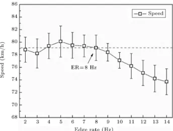
As dened, edge rate equals temporal frequency when the textures are xed (the spatial frequency is con-stant), and it directly relates to the speed and the density of textures. Therefore, the eects of speed and edge rate are examined separately. In fact, edge rate can lead to speed overestimation of drivers, which results in actual speed reduction, and this is supported by Figure 6. Figure 6 shows that the speed decreases when the edge rate increases from 5 Hz to 14 Hz. Specically, when the edge rate falls in [5 Hz,8 Hz], the speed slightly uctuates with a gentle declination; when the edge rate falls in [8 Hz,14 Hz], the speed decreases sharply.
Time headway may change since the speed is reduced due to edge rate from line markings. A one-way ANOVA shows that there is a signicant inuence of edge rate on time headway in the conditions of = 2 m (F (9; 286) = 15:62, p < 0:05) and = 4 m (F (3; 297) = 11:43, p < 0:05), but no signicance is found in the condition of = 8 m (F (2; 304) = 16:71, p = 0:142 > 0:05). Figure 7 demonstrates the changes of time headway along with edge rate in conditions of = 2 m, = 4 m, and = 8 m. In the condition of = 2 m, the time headway rises from 3.79s to 4.39s when the edge rate increases from 5Hz to 12Hz; in the condition of = 4 m, the time headway slightly increases from 4.18s to 4.53s when the edge rate increases from 4 Hz to 7 Hz; but there is no signicant change of time headway in the condition of = 8 m. 3.3. Eects of on time headway
Prior to examining the inuence of on time headway, we check if of line markings can aect the following distance headway directly. Figure 8 demonstrates the average distance headway under dierent speed intervals in each test. It can easily be seen that there are similar variation trends among the tests. That is, under dierent speed intervals, the distance
Figure 7. Mean time headways under dierent edge rate values in test (a), test (b), and test (c).
headways of the three tests are all greater than that of control. Specically, when compared to the control, greater increases are seen in conditions of = 2 m (4:77 m (V < 65 km/h), 3.95 m (65 km/h V 80 km/h), 3.74 m (V > 80 km/h)) and = 4 m (3.82m (V < 65 km/h), 3.86 m (65 km/h V 80 km/h), 3.82 m (v > 80 km/h)) than in the condition of = 8 m (1.74m (V < 65 km/h), 1.87m (65 km/h V 80 km/h), 1.95 m (V > 80 km/h)).
Based on the analysis of distance headway, the eects of on time headway are then examined by one-way analysis of variance (ANOVA). It shows that there is a signicant inuence of on the time headway in general (F (2; 1190) = 27:36; p < 0:05). In addition, the changes in time headway between observation section 1 and observation section 6 in the three tests are found to be signicant (F (2; 1190) = 23:52; p < 0:05). 4. Discussion
In brief, the time headway increases after the in-stallation of line markings. Meanwhile, within the experimental area, the time headway rises with the proceeding of vehicles on the slow lane. Combined with the factor of speed, it is found that the time headway
Figure 8. Mean distance headways under dierent speeds. Here, V is the average speed of each test.
increases with increase in edge rate while the speed decreases.
According to the trac ow theory, the changes in time headway originate from the changes in speed and/or distance. Thus, the increase in time headway may arise from the perception of speed and distance that are aected by the line markings.
4.1. Time headway inuenced by speed perception
Intuitively, we can see that the result in Figure 6 is consistent with the study of Liu et al. [22]. In this study, when the edge rate falls in [5 Hz, 14 Hz], the speed decreases along with the increase in edge rate; in the study of Liu et al. [22], a similar speed reduction occurred as the edge rate increased from 8 Hz to 16 Hz. Though we conducted experiments in a real-world expressway, which was signicantly dierent from the simulation study of Liu, the similar result could be taken from the quantitative relation between perceived and physical variables that were introduced by Shen et al. [18]. Shen et al. [18] introduced the equation Vp = Vn: ft1 n= V:fs1 n(because V = ft=fs), where
Vp is the perceived speed; V is the actual speed; ft
Figure 9. Comparison of speed dierences of all tests.
and n is the undetermined constants. When the speed or the temporal frequency is high enough, parameter n falls in [0,1], i.e. 0 < n < 1. It means that the higher the temporal or spatial frequency is, the greater the speed will be overestimated. More importantly, it is found both in this study and in Liu's study that the speed overestimation leads to the reduction in actual speed. Besides, comparing Figure 7 with Figure 6, it can be found that when the edge rate rises from 5 Hz to 12 Hz, the time headway increases while the speed decreases. This consistency seems to say that the reduction in actual speed, resulted from speed overestimation, may directly lead to the increase in time headway.
In eect, the dierence in perceived speed may cause the change in the speed dierence between leading and following vehicles, which results in the change in time headway. Figure 9 shows the changes in speed dierence of leading and following vehicles, and it can be found that the line markings result in an increase in speed dierence. The eect of on the speed dierence is found to be signicant (F (2; 1190) = 15:28; p < 0:05).
Actually, according to the linear car-following model of steady state [9], xn+1 (t + T ) =
0[ _xn(t) _xn+1(t)], where, xn(t) is the location of
vehicle n at the moment of t; xn(t) is the instantaneous
speed of vehicle n at the moment of t; _xn+1(t + T ) is
the instantaneous acceleration of vehicle n + 1 at the moment of t+T ; and 0is the coecient of sensitivity.
Obviously, it is indicated that the change of speed dierence is the direct reason for the change in time headway. Therefore, the increase in speed dierence ([ _xn(t) _xn+1(t)]) could lead to the increase in time
headway.
4.2. Time headway inuenced by distance perception
The lambda (spatial frequency) of line markings may
have inuences on the estimation of physical distance (i.e., distance headway), which therefore leads to changes in time headway. Firstly, it can be found out from Figures 6 and 7 that when the edge rate is less than 7 Hz, there are no signicant eects of edge rate on speed (F (5; 648) = 14:72; p = 0:102 > 0:05), whereas the time headway keeps on increasing. This oppo-site change indicates that the perception of distance predominates the inuence of line markings on time headway. As shown in Figure 8, the increase in distance headway can be attributed to distance underestimation of drivers in car-following. Actually, this kind of distance underestimation eect is in accordance with that of the previous studies. That is, the \discontinuity eect" can also be found in the situations of high-speed motion, like car-following. Notably, in this study, the visual information is altered by the designed line markings placed along the original markings of the slow lane. Thus, to certain extents, the line markings could be regarded as discontinuous texture on road surface. Therefore, distance underestimation would happen among drivers since the originally continu-ous visual information changes by the designed line markings. Furthermore, because of the \discontinuity eect", drivers have to choose an, at least mentally, relatively safer way to follow. As a consequence, the headway increases.
In addition, Figure 8 also indicates that a high spatial frequency can result in a greater distance headway. Specically, when compared with Figure 4, it can be found that there is a similar relation between time headway and the lambda (spatial frequency) of line markings. Actually, this relation is in line with the study of Fajen [29]. The results of Fajen's virtual-reality experiment demonstrated that the average stop-ping distance decreased with the increase in the density of texture (note that, here, the value of stopping distance was negative because all vehicles exceeded the `STOP' sign). This means that a high spatial frequency can lead to a greater increment in distance headway, which results in the increase in time headway.
Actually, in a micro-perspective of the car-following situation, the driver of the very rst leading vehicle of a platoon meets no other vehicles in his/her stopping distance range, which means he/she does not have to pay too much attention to the distance between the vehicle (if there is any) just ahead and him/her. Therefore, at this moment, the \discontinuity eect" of line markings on his/her distance perception would be relatively limited, but the perceived speed would be still mattered. On the other hand, the following drivers would have to respond to the very rst leading vehicle as its speed reduces. Consequently, the line markings would impact on both the speed perception and the distance perception of the following drivers. Then, the following vehicles would move forward with
a greater deceleration, which results in the increase in time headway.
5. Conclusion
This study examined the eects of perceived speed and perceived distance on time headway in car-following, which might provide evidence for the interpretation of the eects of perceptual variables in the decision and control behavior of car-following. We conducted a series of eld tests and collected real-world data. Statistical analyses showed that the time headway increased, because the perceptions of speed and dis-tance were aected by the designed line markings. This study, to a certain extent, endeavored to develop the visual perception of speed and distance from a static and/or virtual situation into an environment of dynamic motion (car-following). Results in this study explained that the articially designed visual informa-tion could improve the roadway safety by intervening the driving behavior. It means that the line markings could be a new solution to rear-end collisions for the improvement of car-following safety.
However, there were also limitations. Firstly, from the viewpoint of the experimental design, though the greatest increment of time headway was seen when = 2 m, there was not enough evidence to support that there could exist an interval of spatial frequency (or temporal frequency) to which drivers were most sensitive, because only three units ( = 2 m, = 4 m, and = 8 m) of line markings were chosen in the present study. On the other hand, other optical information may also play a role in the process of car-following, such as the optic ow rate, which is related to the eye height of drivers and the size of the leading vehicle. In addition, there may be dierences with regard to gender and age in the perception of speed and distance among drivers, which may result in dierences in time headways.
Therefore, in the future, we will probably focus on nding the design of line markings that can aect the driving behavior most, and on the control of other latent variables like the driver's eye height.
Additionally, the application of the designed line markings can be a \beforehand" countermeasure at accident-prone locations for accident prevention. This \beforehand" countermeasure may decrease the num-ber of accidents or, at least, reduce the intensity of the collision accidents since the line markings force the drivers to adjust their behavior in advance.
Acknowledgements
This work was supported by a grant from the National Natural Science Foundation of China (No. 551078299) and by a grant from the Ministry of Transport of the
People's Republic of China (No. 2010353342240). The authors would like to thank Lingzi Cheng for the help in English writing, and Yu Wu and Huaizhong Zhu for their assistance in the collection of the data used in this study.
References
1. Ministry of Public Security Trac Management Bu-reau. \White paper on road trac accidents in China 2010 ", Trac Management Bureau, P.R.C. Ministry of Public Security, China (2011) (in Chinese). 2. Risto, M. and Martens, M.H. \Time and space: the
dif-ference between following time headway and distance headway instructions", Transportation Research Part F: Trac Psychology and Behaviour, 17, pp. 45-51 (2013).
3. Vogel, K. \A comparison of headway and time to collision as safety indicators", Accident Analysis and Prevention, 35(3), pp. 427-433 (2003).
4. Van Winsum, W. and Heino, A. \Choice of time-headway in car-following and the role of time-to-collision information in braking", Ergonomics, 39(4), pp. 579-592 (1996).
5. Tajeb-Maimon, M. and Shinar, D. \Minimum and comfortable driving headways: reality versus percep-tion", Human Factors: The Journal of the Human Factors and Ergonomics Society, 43(1), pp. 159-172 (2001).
6. Taieb-Maimon, M. \Learning headway estimation in driving", Human Factors: The Journal of the Human Factors and Ergonomics Society, 49(4), pp. 734-744 (2007).
7. Lewis-Evans, B., De Waard, D. and Brookhuis, K.A. \That's close enough{a threshold eect of time head-way on the experience of risk, task diculty, eort, and comfort", Accident Analysis and Prevention, 42(6), pp. 1926-1933 (2010).
8. Brackstone, M. and McDonald, M. \Car-following: a historical review", Transportation Research Part F: Trac Psychology and Behaviour, 2(4), pp. 181-196 (1999).
9. Rothery, R.W. \Car following models", in Revised Monograph on Trac Flow Theory, H. Lieu, Federal Highway Administration, United States of America (2011).
10. Hoogendoorn, S.P. and Botma, H. \Modeling and estimation of headway distributions", Transportation Research Record, 1591, pp. 14-22 (1997).
11. Hoogendoorn, S.P. and Botma, H. \New Estimation technique for vehicle-type-specic headway distribu-tions", Transportation Research Record, 1646, pp. 18-28 (1998).
12. Sivak, M. \The information that drivers use: is it indeed 90% visual?", Perception, 25(9), pp. 1081-1089 (1996).
13. Boer, E.R. \Car following from the driver's perspec-tive", Transportation Research Part F: Trac Psychol-ogy and Behavior, 2(4), pp. 201-206 (1999).
14. Andersen, G.J. and Sauer, C.W. \Optical information for car following: the driving by visual angle (DVA) model", Human Factors: The Journal of the Human Factors and Ergonomics Society, 49(5), pp. 878-896 (2007).
15. Van Winsum, W. \The human element in car follow-ing models", Transportation Research Part F: Trac Psychology and Behaviour, 2(4), pp. 207-211 (1999). 16. Warren, R. \Optical transformations during
move-ment: review of the optical concomitants of egospeed", Report AFOSR-81-0108, Columbus: Ohio State Uni-versity, Department of Psychology, Aviation Psychol-ogy Laboratory (1982).
17. Shen, H., Shimodaira, Y. and Ohashi, G. \Eects of temporal frequency on speed discrimination and perceived speed", International Joint Conference on Neural Networks, Portland, USA, pp. 188-193 (2003). 18. Shen, H., Shimodaira, Y. and Ohashi, G. \Speed-tuned
mechanism and speed perception in human vision", Systems and Computers in Japan, 36(13), pp. 1-12 (2005).
19. Francois, M., Morice, A.H., Bootsma, R.J. and Mon-tagne, G. \Visual control of walking velocity", Neuro-science Research, 70(2), pp. 214-219 (2011).
20. Larish, J.F. and Flach, J.M. \Sources of optical in-formation useful for perception of speed of rectilinear self-motion", Journal of Experimental Psychology. Hu-man Perception and PerforHu-mance, 16(2), pp. 295-302 (1990).
21. Rakha, H.A., Katz, B.J. and Duke, D. \Design and evaluation of peripheral transverse bars to reduce vehicle speeds", 85th Transportation Research Board Annual Meeting, Washington, D.C., USA, 06-0577 (2006).
22. Liu, B., Zhu, S.Y., Wang, H., Xia, J. and Sun, Q.M. \Design theory for speed control by using con-stant edge rate", 9th International Conference of Chi-nese Transportation Professionals (ICCTP), Harbin, China, pp. 419-424 (2009).
23. Gibson, J.J., The Perception of the Visual World., Houghton Miin, Boston, USA (1950).
24. Sinai, M.J., Ooi, T.L. and He, Z.J. \Terrain inu-ences the accurate judgment of distance", Nature, 395(6701), pp. 497-500 (1998).
25. Wu, B., He, Z.J. and Ooi, T.L. \A ground surface based space perception in the virtual environment", Journal of Vision, 2(7), pp. 513-513 (2002).
26. Yarbrough, G.L., Wu, B., Wu, J., He, Z.J. and Ooi, T.L. \Judgments of object location behind an obstacle depend on the particular information selected", Jour-nal of Vision, 2(7), pp. 625-625 (2002).
27. Feria, C.S., Braunstein, M.L. and Andersen, G.J. \Judging distance across texture discontinuities", Per-ception, 32(12), pp. 1423-1440 (2003).
28. AASHTO. A Policy on Geometric Design of Highways and Streets, American Association of State Highway, USA (2011).
29. Fajen, B.R. \Calibration, information, and control strategies for braking to avoid a collision", Journal of Experimental Psychology. Human Perception and Performance, 31(3), pp. 480-501 (2005).
Biographies
Naikan Ding graduated with BS degree in Trac Engineering from Wuhan University of Technology, Wuhan, Hubei, P.R. China, in 2010. Afterwards, he received his MS degree in Transportation Planning and Management from Wuhan University of Technology in 2013. He is now pursuing his PhD in Transportation Planning and Management. His research interests mainly focus on trac safety and driving behavior, with consideration of the driver's visual perceptions. Shunying Zhu, PhD, is a Professor of Trac En-gineering in the School of Transpiration at Wuhan University of Technology. His research interests range from transportation planning and management to trac safety, from drivers to pedestrians, and from fundamental research to applied research. His research has been funded by the National Natural Science of Foundation of China, the Ministry of Transport of People's Republic of China, enterprises, and non-prot organizations.
Hong Wang is an Associate Professor of Road and Bridge Engineering in the School of Transpiration at Wuhan University of Technology. She has been teaching \Road Survey and Design" for fteen years. Her research interests focus on road design theory and method and road safety engineering. Her research links the road design theories to the practical engineering applications.
Nisha Jiao graduated with MS degree in Trans-portation Planning and Management from Wuhan University of Technology in 2012. She is now an Assistant Engineer at Planning Research Studio in the Department of Transportation of Hubei Province, P.R. China, and works on transportation planning and development strategy research of Hubei Province.