Sharif University of Technology
Scientia IranicaTransactions D: Computer Science & Engineering and Electrical Engineering www.scientiairanica.com
Greedy spanner algorithms in practice
M. Farshi
and M.J. Hekmat Nasab
Department of Computer Science, Yazd University, Yazd, P.O. Box 89195-741, Iran.
Received 15 March 2014; received in revised form 21 September 2014; accepted 8 December 2014
KEYWORDS Geometric networks; Euclidean graphs; Geometric spanners; Greedy algorithm; Greedy spanner.
Abstract. Spanners generated by the greedy algorithm - or greedy spanners - not only have good theoretical properties, like a linear number of edges, low degree and low weight, but also, as previous experimental results show, they are superior to spanners generated by other algorithms in practice. Because of the good properties of greedy spanners, they found several applications like in protein visualization.
The major issue in computing greedy spanners is the high time and space complexity of algorithms that compute it. To construct the greedy spanner on a set of n points, the original greedy algorithm takes O(n3log n) time. In 2005, an improvement was proposed by
Farshi and Gudmundsson [Lecture Notes in Computer Science, Vol. 3669, pages 556-567] that works much faster in practice, but later it was shown that it has same theoretical time complexity. In 2008, Bose et al. [Lecture Notes in Computer Science, Vol. 5124, pages 390-401] discovered a near-quadratic time algorithm for constructing greedy spanners. In this paper, we compare time complexity of these three algorithms for computing the greedy spanner in practice.
c
2014 Sharif University of Technology. All rights reserved.
1. Introduction
A network on a set V of n points (in Euclidean space) can be modeled as an undirected graph G with vertex set V of size n and an edge set E of size m where every edge e = (u; v) has a weight wt(e). A network is called a geometric or Euclidean network if the weight of the edge e = (u; v) is the Euclidean distance juvj between its endpoints u and v.
There are several ways to measure the quality of a network; one is the dilation or stretch factor of the network. For each pair of points u; v 2 V , the ratio of the length of the shortest path between u and v in G, denoted by dG(u; v), to the Euclidean distance
between u and v is called the dilation between u and v in G. The length along a path is sum of lengths of *. Corresponding author. Tel.: +98 35 31232689;
Fax: +98 35 38210695
E-mail addresses: [email protected] (M. Farshi); [email protected] (M.J. Hekmat Nasab)
all edges on the path. The maximum dilation between all pairs of vertices of G is called the dilation of G. Informally, in a network with low dilation, the amount of detour one might need to take to travel from one node to another node of the graph, when it is only allowed to travel along edges of the graph, is close to the actual Euclidean distance between the nodes.
Let t 1 be a real number. A network G is called a t-spanner on vertices of G, if the dilation of G is at most t. In other words, a graph G(V; E) is a t-spanner of V , if for each pair of vertices u; v 2 V , there exists a path in G between u and v of weight at most t juvj. We call such a path a t-path between u and v.
Obviously, with this measure of quality, we need to have a lot of edges in the graph to have good networks which means they are expensive to build. So the main objective of studying spanners is to construct sparse t-spanners with t suciently close to 1. To measure sparseness, one can consider dierent criteria like the weight of the spanner, i.e. sum of weights of all of its edges, the number of edges and the maximum
degree. Spanners have applications in several elds: from robotics, network topology design, distributed systems and design of parallel machines to metric space searching [1], protein visualization [2] and broadcasting in communication networks [3].
There are several algorithms that given a set of points and a t > 1, compute a t-spanner of the point set in Rd (see [4]). Dierent algorithms generate spanners
with dierent properties, most of them contain a linear number of edges, and some of them have low weight and degree. Next to theoretical results, algorithms are compared in experiments based on dierent properties, like number of edges, maximum degree and weight of generated graph and also the running time of them (see [1,5,6]).
The greedy algorithm is not only the simplest algorithm to generate a spanner, but the generated spanners also have a linear number of edges, constant degree and optimal weight in theory. Experiments also show that the greedy algorithm generates spanners which have superior properties compared to other algorithms [5]. The only problem with the algorithm is its time and space complexity, the original greedy algorithm requires cubic time and quadratic space complexity which makes it impossible to compute the greedy spanner. Greedy spanner is generated by the greedy algorithm, on sets of points that contain more than a few thousand points using the original greedy algorithm. In [5] Farshi and Gudmundsson proposed an improvement (we will refer to the improved variant as FG-Greedy) that worked well in practice, however, it was later shown [7] that this improvement does not improve the theoretical worst-case bound. In the same paper, Bose et al. introduced an algorithm that gener-ates the greedy spanner in O(n2log n) time using O(n2)
space. To the best of our knowledge, this algorithm had not been implemented before (Independently of our work, Bouts et al. [8] have recently implemented this algorithm).
Recently, Alewijnse et al. [9] proposed an algorithm that computes the greedy spanner in O(n2log2n) time using linear space (note that all
previous greedy algorithms use quadratic space). They also implemented the algorithm and showed the prac-tical behaviour of the algorithm on point sets with dif-ferent distributions and up to one million points which was a big progress since the highest number of points that the greedy spanner generated before this contains only 13,000 points [5]. They also showed that the expected time complexity of their algorithm is linear for uniformly distributed point sets. There is also another recent and independent work by Bouts et al. [8] that provides a theoretical framework for analyzing greedy spanner algorithms. In particular it provides improved analytical bounds for two of the algorithms discussed in this paper. For the FG-Greedy algorithm it provides
a bound in terms of the spread of the point set; this resolves the question why the FG-Greedy performs well in practise and also explains its performance in the experiments on uniformly distributed data. For NQT-Greedy, the paper proves a tighter bound in terms of t. It also reports on some experiments on the three algorithms discussed in this paper.
In this paper we compare the Bose et al. greedy algorithm with two other algorithms that generate greedy spanner, based on their running time in prac-tice. We did not consider the linear space algorithm introduced by Alewijnse et al. [9].
We should mention that there exist an algorithm with near-linear worst-case time complexity, namely approximate greedy algorithm [4,10], that generates spanners with theoretical properties similar to the greedy spanner but, as previous experiments show (see [5]) in practice it is far worse than the greedy spanner especially when t is close to 1 and points are uniformly distributed.
The paper is organized as follows. First we briey describe the implemented algorithms together with the theoretical bounds and implementation details. In Section 3 we discuss the experimental results. Finally, we discuss possible improvements and future research. Throughout the paper, t will be assumed to be a small constant. In the experiments we used values of t between 1.02 and 2, because in most applications t is close to 1. Also for larger values of t there are other options like the Delaunay triangulation which is known to have dilation 1:998 [11]. Also, we know that any 2-spanner is a t-spanner for each t > 2.
2. Greedy spanner algorithms
Here, we give a short description of each of the algorithms implemented together with their theoretical bounds. For a detailed description of each algorithm, considered in this section, please refer to the book by Narasimhan and Smid [4] and papers by Farshi and Gudmundsson [5], Bose et al. [7] and Bouts et al. [8]. 2.1. The original greedy algorithm
The greedy algorithm was introduced independently by Althofer et al. [12] and Bern in 1989, and since then, other researchers worked on it (see [10,13-17]). The graph constructed using the greedy algorithm will be called a greedy graph or a greedy spanner. Note that, as we will see, if no pair of points in the input set has same distance, then the greedy spanner is unique. Otherwise, we can have several greedy spanners. But, if we x an order on pairs with equal distances, then again we can assume that the greedy spanner is unique. Intuitively, the original greedy algorithm con-structs the graph in a natural way, like producing the road network between cities generated by humans. It
starts to check cities that are close to each other and adds a road between them if there is no short route between them on existing roads, and continues to check pairs that are farther apart. More formally, the original algorithm starts with a graph with no edges. Then, it considers all pairs of points in increasing order based on the distance between a pair of points. In other words, it sorts all pairs of points with respect to their increasing distances, and then processes them in that order. To process an edge (u; v), it performs a shortest path query in G between u and v, and if there is no t-path between u and v in G, i.e. the length of the shortest path between u and v is more than t:juvj, then (u; v) is added to G, otherwise it is discarded. Since the original greedy algorithm checks n
2
pairs of points, and for each pair, it performs one shortest path query (using Dijkstra's algorithm implemented by Fibonacci heap), which takes O( n
t 1+ n log n) time (since there
are O( n
t 1) edges in G), the time complexity of the
algorithm is O(n3
t 1+ n3log n) and it uses O(n2) space.
The greedy approach can also be used to prune a given graph G = (V; E), that is, instead of considering all pairs of points (see Algorithm 1), the algorithm only considers those which are endpoints of the edges in E. 2.2. The FG-greedy algorithm
Because of the cubic time complexity of the original greedy algorithm, it is practically impossible to
con-struct greedy spanner on point sets with more than a few thousand points. For example, based on the ex-periments in [5,18], constructing the greedy 2-spanner on a set of 4,000 uniformly distributed points in the Euclidean plane, using the original greedy algorithm, takes more than 12,000 seconds and constructing 1:1-spanner on the same point set takes almost 42,000 seconds.
To make it possible to do experiments on larger point sets, Farshi and Gudmundsson [5,18] proposed a simple technique to improve the running time of the original greedy algorithm. The new algorithm, which we will call FG-greedy algorithm, works similar to the original greedy algorithm, except it uses a matrix to store the length of the shortest path between pairs of points. The matrix is updated when the algorithm performs a single-source shortest path query. Each time the algorithm wants to check if there is a t-path between a pair of points, it rst checks the matrix to see if the path length between the points is less than t times the Euclidean distance between the points. If the path length is small enough, it skips the edge without performing the single-source shortest path query. Otherwise, it performs the shortest path query and then it updates the distance matrix and then decides whether the edge should be added to the graph or not (see Algorithm 2). Note that the distance matrix is not up-to-date, so if the distance
Algorithm 1. The original greedy algorithm.
between a pair of points is not small enough, it updates the matrix for the pair of points and then makes its decision.
As experiments show, [5,18], this improved algo-rithm uses around 35 and 100 seconds to compute 2-spanner and 1:1-2-spanner on a set of 4,000 uniformly distributed points which shows a big improvement. Using this improvement, the greedy spanner on point sets containing up to 13,000 points was constructed.
Note that, as shown by Bose et al. [7], this im-provement does not improve the worst-case theoretical time complexity of computing greedy spanners. 2.3. The NQT-greedy algorithm
In 2008, Bose et al. [19] proposed a near-quadratic time algorithm to compute the greedy spanner which was based on the FG-greedy algorithm. Their algorithm makes the following changes. It partitions the n
2
pairs of distinct points in V into buckets, such that within each bucket, distances dier by at most a factor of two; then, the algorithm processes the buckets one after another.
Consider the current bucket contains all pairs whose distances are in the interval [L; 2L). For each point u of V , it performs the bounded Dijkstra's algorithm with source u and distance 2tL, and stores all operations performed by the Dijkstra's algorithm in a stack. Thus, for each vertex v, such that dG(u; v)
2tL, the value of dG(u; v) is known, which is stored
as weight(u; v) in the distance matrix. When the algorithm adds an edge (u; v) to the greedy spanner, it takes all points, p, for which the distance between p and one of the endpoints of the edge (u; v) is less than (t 1
2)L and updates corresponding distances. To
update the distances, instead of running the bounded Dijkstra's algorithm with source p and distance 2tL from scratch, it uses the stack stored with p to undo the execution of the bounded Dijkstra's algorithm (in the graph prior to the insertion of the edge (u; v)) until the minimum key in the priority queue is at most min((t 1
2)L; L). Then, it restarts Dijkstra's algorithm
from this state, using the graph that contains the new edge (u; v), and terminate as soon as the minimum key in the priority queue is larger than 2tL; during the execution, it stores the sequence of all operations in the stack associated with p.
A detailed description of the algorithm is given in Algorithms 3-5. The time complexity of this algorithm is O(n2log n) and it uses O(n2) space [7].
2.3.1. Implementation
The implementations of the rst two algorithms are straight-forward. Implementing the third algorithm is a bit tricky, because of the undo/redo operations that have to be done when performing the Dijkstra's algorithm. We used some (extra) data structures to
be able to do this operation without increasing the complexity of the algorithm.
We implemented the algorithms in C++ and compiled the code using -o argument. The data structures needed were implemented using the pseudo-codes of [20], some of which are with minor changes. To keep the graph, we used an adjacency matrix and to be able to nd all neighbours of a vertex, we also kept all neighbours of each vertex in a linked list. Using this, we can check adjacency between vertices in constant time and we can traverse all neighbours of a vertex in time proportional to the degree of the vertex. The priority queue is implemented using a min-heap (see [20]), and to make it possible to nd an specic vertex in the priority queue in constant time, we maintain an array of pointers which keep a pointer to vertex i in the priority queue in its ith entry of the array. The stack is implemented using a linked list. For the list of pairs of points, we use a structure that stores indices of the points with their Euclidean distance.
The experiments were done on two dierent ma-chines. For point sets up to 4,000 points in the Euclidean plane, the code is compiled using G++ version 4.6 and runs on a Intel E2200 (2.2 GHz x2) machine with 3 GB of RAM and Ubuntu 12.04 operating system. For larger point sets, we needed more memory, so we ran the code on a Intel Xeon E5620 (2.4 GHz) with 24 GB RAM and Debian 6.0.3 operating system and G++ version 4.4.
The experiments are done on uniformly dis-tributed point sets; for point sets up to 4,000 points the range of each coordinate is between 0 and 10,000, and for larger point sets, the range of each coordinate is between 0 and 30,000. For each case, we run the algorithms on 3 to 10 dierent point sets and we take average between them and use maximum and minimum values between them to see how much the dierence between dierent point sets is.
Note that all algorithms mentioned here produce exactly the same networks, so we do not need to com-pare the networks generated by dierent algorithms. 3. Running time comparison
The results of the experiments are presented in Ta-bles 1, 2 and 3 for dierent point sets and dierent t's. The time in all tables and diagrams are in seconds.
The rst thing one can see in the tables is that the FG-greedy is faster than NQT-greedy algorithm in practice for all t's which are big enough. We expected this result, since the amount of overhead of the NQT-greedy algorithm is higher than the FG-greedy algorithm.
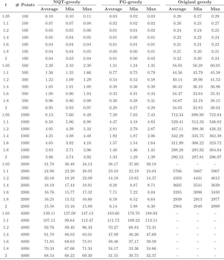
But, for low values of t, as shown in Figure 1, the NQT-greedy algorithm runs faster than the FG-greedy algorithm. The improvement is 50 percent for t = 1:02
Algorithm 3. The Near-Quadratic Time (NQT) greedy algorithm.
Algorithm 5. The algorithm to undo previous operations of the Dijkstra's algorithm.
Table 1. The running time (in seconds) of dierent greedy algorithms for dierent t's and point sets up to 4,000 points.
t # Points NQT-greedy FG-greedy Original greedy
Average Min Max Average Min Max Average Min Max
1.05 100 0.10 0.10 0.11 0.03 0.02 0.03 0.28 0.27 0.29
1.1 100 0.07 0.07 0.08 0.02 0.02 0.02 0.26 0.25 0.27
1.2 100 0.05 0.05 0.06 0.01 0.01 0.02 0.24 0.24 0.25
1.4 100 0.05 0.04 0.05 0.01 0.00 0.01 0.23 0.22 0.24
1.6 100 0.04 0.04 0.04 0.01 0.01 0.01 0.21 0.21 0.22
1.8 100 0.04 0.04 0.05 0.00 0.00 0.01 0.21 0.20 0.21
2 100 0.04 0.03 0.04 0.01 0.00 0.02 0.22 0.20 0.24
1.05 500 2.30 2.10 2.38 1.31 1.24 1.35 58.85 56.28 60.05
1.1 500 1.56 1.35 1.66 0.77 0.75 0.79 44.56 43.79 45.58
1.2 500 1.22 1.09 1.29 0.54 0.52 0.58 40.14 38.90 41.53
1.4 500 1.05 1.01 1.08 0.38 0.36 0.39 36.42 36.10 36.86
1.6 500 1.00 0.96 1.04 0.32 0.31 0.34 34.47 33.84 35.31
1.8 500 0.96 0.90 0.98 0.30 0.28 0.31 34.87 33.19 38.15
2 500 0.95 0.93 0.97 0.28 0.27 0.29 34.05 32.83 38.02
1.05 1000 8.13 7.60 8.49 7.29 7.02 7.43 712.34 698.98 722.84
1.1 1000 6.50 5.96 6.98 4.47 4.18 4.83 529.41 512.33 546.82
1.2 1000 4.95 4.39 5.32 2.81 2.79 2.87 407.11 398.36 426.22
1.4 1000 4.25 4.08 4.48 1.92 1.87 2.06 342.29 335.75 362.38
1.6 1000 4.05 3.92 4.10 1.57 1.54 1.64 311.99 306.22 323.72
1.8 1000 3.83 3.71 3.96 1.40 1.36 1.45 298.28 295.92 304.04
2 1000 3.86 3.74 3.92 1.33 1.29 1.39 290.52 287.81 296.97
1.05 2000 31.78 30.48 34.13 38.17 37.60 39.18 - -
-1.1 2000 24.98 23.20 28.02 23.10 22.19 24.04 5766 5667 5907
1.2 2000 20.16 18.28 22.09 14.18 13.85 14.37 4503 4431 4612
1.4 2000 18.19 17.44 18.91 9.28 8.87 9.71 3605 3541 3639
1.6 2000 16.76 15.77 17.32 7.71 7.22 8.04 3285 3096 3450
1.8 2000 16.25 15.52 16.60 6.59 6.52 6.64 2939 2913 2977
2 2000 15.58 15.16 15.89 6.14 5.98 6.30 2904 2849 2999
1.05 4000 139.11 127.08 147.13 183.60 179.70 188.93 - -
-1.1 4000 107.15 99.64 112.47 111.72 109.23 113.11 - -
-1.2 4000 92.76 89.40 96.43 70.27 68.84 72.31 - -
-1.4 4000 81.78 80.03 83.01 47.09 46.26 47.69 - -
-1.6 4000 71.85 69.63 75.01 38.46 37.17 39.59 - -
-1.8 4000 70.34 67.66 71.34 34.17 33.36 34.66 - -
-Table 2. The running time (in seconds) of dierent greedy algorithms for dierent t's and point sets between 4,000 and 10,000 points.
# Points t NQT-greedy FG-greedy
Average Min Max Average Min Max
4000 1.2 79.16 71.01 82.58 52.21 50.69 53.14
5000 1.2 125.99 117.36 132.01 97.25 95.49 98.51 6000 1.2 189.66 172.03 210.59 141.62 138.16 144.86 8000 1.2 341.87 300.64 369.78 272.96 262.92 288.20 10000 1.2 552.69 503.64 588.29 454.21 445.26 461.40
4000 1.6 64.94 62.61 66.01 30.86 30.26 31.16
5000 1.6 100.85 96.85 106.63 51.03 50.61 52.25 6000 1.6 154.50 147.87 156.55 75.44 74.99 76.41 8000 1.6 271.16 257.74 284.87 145.73 142.05 151.29 10000 1.6 445.26 423.18 459.23 245.15 241.75 249.70
4000 2 58.27 57.22 59.71 25.43 24.87 25.90
5000 2 94.62 92.88 95.91 41.49 41.10 41.91
6000 2 140.05 137.80 141.40 61.55 60.84 62.41 8000 2 252.35 245.62 259.85 119.15 116.86 121.22 10000 2 408.48 400.75 412.49 199.58 195.75 201.54
Table 3. The running time (in seconds) of dierent greedy algorithms for t = 1:1 and point sets between 4,000 to 12,000 points.
# Points NQT-greedy FG-greedy
Average Min Max Average Min Max
4000 92.69 81.87 99.2 80.23 79.47 81.59
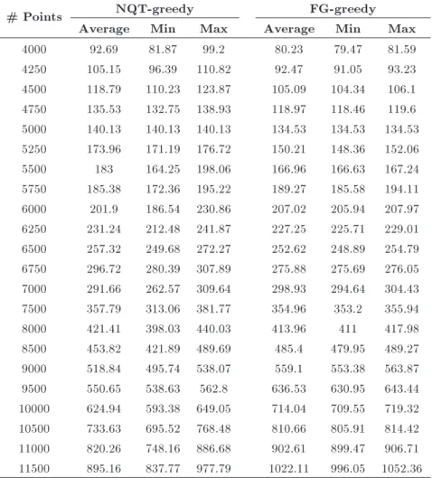
4250 105.15 96.39 110.82 92.47 91.05 93.23 4500 118.79 110.23 123.87 105.09 104.34 106.1 4750 135.53 132.75 138.93 118.97 118.46 119.6 5000 140.13 140.13 140.13 134.53 134.53 134.53 5250 173.96 171.19 176.72 150.21 148.36 152.06 5500 183 164.25 198.06 166.96 166.63 167.24 5750 185.38 172.36 195.22 189.27 185.58 194.11 6000 201.9 186.54 230.86 207.02 205.94 207.97 6250 231.24 212.48 241.87 227.25 225.71 229.01 6500 257.32 249.68 272.27 252.62 248.89 254.79 6750 296.72 280.39 307.89 275.88 275.69 276.05 7000 291.66 262.57 309.64 298.93 294.64 304.43 7500 357.79 313.06 381.77 354.96 353.2 355.94 8000 421.41 398.03 440.03 413.96 411 417.98 8500 453.82 421.89 489.69 485.4 479.95 489.27 9000 518.84 495.74 538.07 559.1 553.38 563.87 9500 550.65 538.63 562.8 636.53 630.95 643.44 10000 624.94 593.38 649.05 714.04 709.55 719.32 10500 733.63 695.52 768.48 810.66 805.91 814.42 11000 820.26 748.16 886.68 902.61 899.47 906.71 11500 895.16 837.77 977.79 1022.11 996.05 1052.36
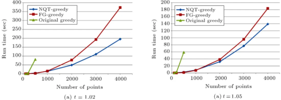
Figure 1. Comparing running time of the greedy algorithms for t = 1:02 and t = 1:05 for point sets up to 4,000 points.
Figure 2. Comparing running time of the greedy algorithms for t = 1:1.
Figure 3. Comparing running time of the greedy algorithms for t = 1:6.
on a point set with 4,000 uniformly distributed points, and for t = 1:05, this improvement is 40 seconds on the same set.
As shown in Figure 2 and Table 3, the FG-greedy and the NQT-greedy algorithm take almost the same time, but the NQT-greedy runs faster for large enough point sets, say sets of more than 8,000 points.
For larger values of t, say t 1:2, the FG-greedy algorithm is faster, and the dierence increases when t grows. However, as one can see in Figures 3 and 4, the running time of the NQT-greedy algorithm grows slower than the running time of the FG-greedy algorithm, which means that one can expect that the NQT-greedy algorithm works faster if the point set is large enough, say with a few million points which is
consistent with the analytical bounds of the algorithms on uniformly distributed points. We were not able to do experiments on larger point sets because they would have needed a lot of memory. For applica-tions with large point sets, the space complexity is one of the major bottlenecks, so we suggest to use an algorithm with linear-space complexity introduced recently (see [8,9]). The time complexity of this linear-space algorithm is slightly more than the NQT-greedy algorithm, but because of its low space complexity, it works much better on large point sets.
From the application perspective, one might want to know, for his special case, which algorithm works faster. To see this, based on experiments, there is a diagram in Figure 5, which shows which algorithm
Figure 4. Comparing running time of the greedy algorithms for t = 2.
Figure 5. In the cases above the graph, the NQT-greedy algorithm runs faster than the FG-greedy algorithm.
works faster based on the number of points and the value of t. In all cases that lie below the graph, the FG-greedy algorithm runs faster and above the graph the NQT-greedy algorithm runs faster.
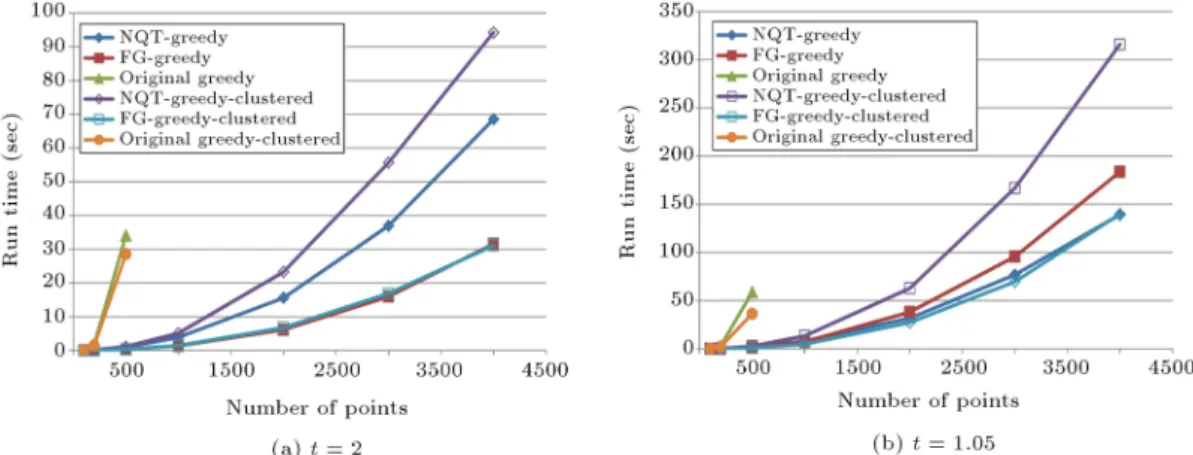
To see how sensitive are the greedy algorithms to the distribution of input point sets, we tested the algorithms on clustered point sets too. To make a clustered point set with n points, we selected pn
uniformly distributed squares and in each square we put pn points. As seen in Figure 6, the FG-greedy algorithm works almost the same for uniform and clustered point sets for t = 2. For lower values of t, say t = 1:05, the FG-greedy algorithm is faster on clustered point sets. However, the NQT-greedy algorithm is slower on clustered point sets and as t decreases, the dierence between running time of the algorithm on uniformly distributed point sets and clustered point sets increases. As seen in Table 4, the ratio of the time used by the NQT-greedy algorithm to the time used by the FG-greedy algorithm decreases when we decrease t or increase n. However, its decrease rate is small, but one can expect that for suciently large point sets and for low values of t, the NQT-greedy algorithm runs faster than the FG-greedy algorithm.
4. Space usage comparison
As seen in the algorithms, the FG-greedy algorithm needs more space compared to the original greedy algorithm, since it uses a matrix to store distance between all pairs of points in the generated graph.
Figure 6. Comparing running time of the greedy algorithms for t = 2 and t = 1:05 between uniformly distributed and clustered point sets.
Table 4. The running time (in seconds) of dierent greedy algorithms for clustered point sets (1st and 2nd columns) and the ratio between them (3rd column).
t # Points NQT-greedy FG-greedy NQT-greedy/FG-greedy
1.05 1000 13.35 4.83 2.76
1.05 2000 62.82 27.30 2.30
1.05 3000 166.79 69.66 2.39
1.05 4000 315.82 139.89 2.26
1.1 1000 9.88 3.44 2.87
1.1 2000 44.44 19.86 2.24
1.1 3000 105.89 45.49 2.33
1.1 4000 202.25 87.90 2.30
1.4 1000 5.37 1.81 2.96
1.4 2000 25.40 9.86 2.58
1.4 3000 59.70 23.09 2.59
1.4 4000 107.88 43.85 2.46
1.8 1000 4.96 1.46 3.40
1.8 2000 22.72 7.20 3.16
1.8 3000 49.97 17.96 2.78
1.8 4000 93.61 32.38 2.89
2 1000 5.09 1.46 3.50
2 2000 23.26 6.75 3.44
2 3000 55.68 16.85 3.30
2 4000 94.24 31.12 3.03
Table 5. The space usage of dierent greedy algorithms for dierent t's and point sets up to 4,000 points. # Points Algorithm t = 1:05 t = 1:1 t = 1:2 t = 1:5 t = 2
n = 2000
Original greedy 61.6 MB 61.5 MB 61.4 MB 61.4 MB 61.3 MB FG greedy 92.2 MB 92.0 MB 92.0 MB 91.9 MB 91.9 MB NQT greedy 547.8 MB 511.7 MB 479.6 MB 451.7 MB 440.9 MB n = 4000 FG greedy 367.3 MB 367.1 MB 366.9 MB 366.8 MB 366.7 MB
NQT greedy 2.2 GB 2 GB 1.9 GB 1.8 GB 1.7 GB
The NQT-greedy algorithm uses extra space to keep all operations performed by Dijkstra's algorithm with source at any point to be able to make undo and xing the shortest path computation after adding an edge to the graph. It is therefore expected that this algorithm uses a large amount of memory. As shown in Table 5, the experiment shows this behaviour, but the memory used by the NQT-greedy algorithm is much more than what is expected. Based on the experiments, memory usage of the FG-greedy algorithm is 1:5 times the memory used by the original greedy algorithm. This amount blows up to 5-6 times more space when using the NQT-algorithm. So the main obstacle of using the
NQT-greedy algorithm is its memory usage, and any improvement on this will be the main interesting future work.
5. Future works
As for future works, one can study improving the space complexity of the NQT-greedy algorithm, or improving the worst-case time complexity of one of the recently introduced linear-space algorithms, see [8,9,21]. An-other interesting question is to design an algorithm for constructing the greedy spanner in I/O-model which is an interesting model for processing big data.
Acknowledgements
The authors would like to thank Mohammad Reza Hooshmand Asl, head of the laboratory of quantum information processing of Yazd university, for giving them access to the Lab's server for doing part of the experiments and the anonymous referees for many insightful comments.
References
1. Navarro, G. and Paredes, R. \Practical construction of metric t-spanners", 5th Workshop on Algorithm Engineering and Experiments, SIAM Press, pp. 69-81 (2003).
2. Russel, D. and Guibas, L.J. \Exploring protein folding trajectories using geometric spanners", Pacic Sympo-sium on Biocomputing, pp. 40-51 (2005).
3. Li, X.-Y. \Applications of computational geometry in wireless ad hoc networks", Ad Hoc Wireless Network-ing, Kluwer (2003).
4. Narasimhan, G. and Smid, M., Geometric Spanner Networks, Cambridge University Press, UK (2007).
5. Farshi, M. and Gudmundsson J. \Experimental study of geometric t-spanners", Journal of Experimental Algorithmics, 14, pp. 3:1.3-3:1.39 (2010).
6. Sigurd, M. and Zachariasen, M. \Construction of minimum-weight spanners", 12th Annual European Symposium on Algorithms, volume 3221 of Lecture Notes in Computer Science, Springer-Verlag, pp. 797-808 (2004).
7. Bose, P., Carmi, P., Farshi, M., Maheshwari, A. and Smid, M. \Computing the greedy spanner in near-quadratic time", Algorithmica, 58(3), pp. 711-729 (2010).
8. Bouts, Q.W., ten Brink, A.P. and Buchin, K. \A framework for computing the greedy spanner", 30th Annual ACM Symposium on Computational Geome-try, pp. 11:11-11:19 (2014).
9. Alewijnse, S.P.A., Bouts, Q.W., Brink, A.P. and Buchin, K. \Computing the greedy spanner in linear space", 21th Annual European Symposium on Algo-rithms, volume 8125 of Lecture Notes in Computer Science, pp. 37-48 (2013).
10. Das, G. and Narasimhan, G. \A fast algorithm for constructing sparse Euclidean spanners", International Journal of Computational Geometry and Applications, 7, pp. 297-315 (1997).
11. Xia, G. \The stretch factor of the Delaunay triangula-tion is less than 1.998", SIAM Journal on Computing, 42, pp. 1620-1659 (2013).
12. Althofer, I., Das, G., Dobkin, D.P., Joseph, D. and Soares, J. \On sparse spanners of weighted graphs", Discrete and Computational Geometry, 9(1), pp. 81-100 (1993).
13. Chandra, B. \Constructing sparse spanners for most graphs in higher dimensions", Information Processing Letters, 51(6), pp. 289-294 (1994).
14. Chandra, B., Das, G., Narasimhan, G. and Soares, J. \New sparseness results on graph spanners", In-ternational Journal of Computational Geometry and Applications, 5, pp. 124{144 (1995).
15. Das, G., Heernan, P.J. and Narasimhan, G. \Op-timally sparse spanners in 3-dimensional Euclidean space", 9th Annual ACM Symposium on Computa-tional Geometry, pp. 53-62 (1993).
16. Gudmundsson, J., Levcopoulos, C. and Narasimhan, G. \Improved greedy algorithms for constructing sparse geometric spanners", SIAM Journal on Com-puting, 31(5), pp. 1479-1500 (2002).
17. Soares, J. \Approximating Euclidean distances by small degree graphs", Discrete and Computational Geometry, 11, pp. 213-233 (1994).
18. Farshi, M. and Gudmundsson, J. \Experimental study of geometric t-spanners", 13th Annual European Sym-posium on Algorithms, volume 3669 of Lecture Notes in Computer Science, Springer-Verlag, pp. 556-567 (2005).
19. Bose, P., Carmi, P., Farshi, M., Maheshwari, A. and Smid, M. \Computing the greedy spanner in near-quadratic time", 11th Scandinavian Workshop on Algorithm Theory, volume 5124 of Lecture Notes in Computer Science, Springer-Verlag, pp. 390-401 (2008).
20. Cormen, T.H., Leiserson, C.E., Rivest, R.L. and Stein, C., Introduction to Algorithms, MIT Press and McGraw-Hill, 2nd edition (2001).
21. Alewijnse, S.P.A., Bouts, Q.W., ten Brink, A.P. and Buchin, K. \Distribution-sensitive construction of the greedy spanner", CoRR, abs/1401.1085 (2014).
Biographies
Mohammad Farshi recieved his BSc in Computer Science from Yazd University, Yazd, Iran in 1996 and his MSc in Pure Mathematics from Shiraz University, Shiraz, Iran, in 1999, and his PhD in Computer Science from Eindhoven University of Technology, Eindhoven, The Netherlands, in 2008. Between 1999 and 2004, he worked at Yazd University as an instructor and from 2009 he has been an Assistant Professor at the same university. His research interests are Computational Geometry, Geometric Spanners and Algorithms. Mohammad Javad Hekmat Nasab received his BSc in Computer Science from Yazd University, Yazd, Iran in 2013. Now he is a Master student at Depart-ment of Mathematics and Computer Science, Amirk-abir University of Technology, Tehran, Iran.