Sharif University of Technology
Scientia IranicaTransactions B: Mechanical Engineering www.scientiairanica.com
Research Note
Optimal tracking control of an underactuated container
ship based on direct Gauss pseudospectral method
M.T. Ghorbani and H. Salarieh
School of Mechanical Engineering, Sharif University of Technology, Tehran, P.O. Box 111559567, Iran. Received 10 September 2012; received in revised form 18 January 2014; accepted 9 March 2014
KEYWORDS Optimal control; Tracking; Ship control;
Gauss pseudospectral transcription; Nonlinear programming.
Abstract. In this paper, the problem of optimal tracking control for a container ship is addressed. The multi-input-multi-output nonlinear model of the S175 container ship is well established in the literature and represents a challenging problem for control design, where the design requirement is to follow a commanded maneuver at a desired speed. To satisfy the constraints on the states and control inputs of the vessel nonlinear dynamics and minimize the heading error, a nonlinear optimal controller is formed. To solve the resulted nonlinear constrained optimal control problem, the Gauss Pseudospectral Method (GPM) is used to transcribe the optimal control problem into a Nonlinear Programming Problem (NLP) by discretization of states and controls. The resulted NLP is then solved by a well-developed algorithm known as SNOPT. The results for keeping and course-changing autopilots illustrate the eectiveness of the proposed approach in dealing with vessel tracking control.
© 2014 Sharif University of Technology. All rights reserved.
1. Introduction
The problem of the tracking control of marine vehicles is a highly important issue, especially for autopilot de-sign. There are some challenges in this area. The rst is that the vessels are often underactuated. Advanced techniques in the eld of control of underactuated systems [1-3] have been suggested for path planning of a 3-DoF vessel (surge, sway and yaw motion) with two independent inputs.
Another diculty for the tracking control of marine surface vessels is the intrinsic physical lim-itations in the control inputs. The rudder deec-tion angle and its rate have operating limits which should be considered. In addition, the controller must
*. Corresponding author. Tel.: +98 21 66165538; Fax: +98 21 66000021
E-mail addresses: mt [email protected] (M.T. Ghorbani); [email protected] (H. Salarieh)
consider safety constraints. Since the roll motion of the marine vehicle is the principal cause for the probabilities of slamming and deck wetness [4], en-forcing roll constraints while maneuvering in seaways becomes an important designation in surface vessel control.
To overcome the mentioned challenges, some control design methods have been developed. Li et al. (2009) used Model Predictive Control (MPC) to control both the cross tracking and heading error by the rudder angle for an underactuated surface vessel while considering rudder limitation and roll constraints [5]. MPC can handle underactuated problems by combin-ing all the objectives into a scombin-ingle objective function. However, due to computational complexity, the MPC applications for systems with fast dynamics are not very common [6]. In addition, Li et al. (2009) used a reduced order linear model for MPC implementation. In general, the linear models result in the loss of vital mathematical information from the dynamics of the
physical systems, and their valid range of operation is small. A better choice to tackle tracking control prob-lems, while satisfying the input and state constraints, is nonlinear optimal control. Nonlinear optimal control satises any of the desirable constraints, and is also suitable for nonlinear systems [7]. In an optimal control problem, the goal is determination of the states and controls that minimize a cost functional subject to nonlinear dynamic constraints, boundary conditions and inequality path constraints. There are two meth-ods for resolving optimal control problems: direct and indirect [8]. In an indirect method, rst-order necessary conditions for optimality are derived from the optimal control problem via the calculus of variations and Pontryagin's minimum principle [9]. These neces-sary conditions form a Hamiltonian Boundary-Value Problem (HBVP), which is then solved numerically for extremal trajectories. The optimal solution is then found by choosing the extremal trajectory with the lowest cost. The primary advantages of indirect methods are high accuracy in the solution and the assurance that the solution satises the rst-order optimality conditions. However, indirect methods have several disadvantages. First, the solution of HBVP must be usually derived analytically, which can be often non-trivial. Second, if one wishes to obtain the solution numerically, as numerical techniques used in indirect methods typically have small radii of convergence, an extremely good initial guess of the unknown solution or boundary conditions is generally required. Finally, for problems with path constraints, it is necessary to have a priori knowledge about the constrained and unconstrained arcs or switching structure [10]. Cimen and Banks (2004) used the indirect method to solve nonlinear optimal tracking control of an oil tanker [7].
On the other hand, the direct methods trans-form the optimal control problem into a nonlinear programming problem (NLP). Direct methods have the advantage that the rst-order necessary condi-tions do not need to be derived. Furthermore, they have much larger radii of convergence than indirect methods and, thus, do not require as good an initial guess. Lastly, the switching structure does not need to be known a priori [10]. In this paper, to solve a nonlinear 4-DoF tracking control problem for an underactuated container ship, we address a kind of direct method, known as the Gauss Pseudospectral Method (GPM), to transform the optimal control problem into an NLP by parameterization of the states and the controls. These parameterization techniques have an important role to play in the convergence and accuracy of the solution, and low computation time [11]. The resulted NLP is then solved by a well-developed algorithm called SNOPT. The proposed method is suitable for autopilot design and provides
tracking of a commanded course heading at a desired shaft velocity, while satisfying the roll and rudder constraints.
This paper is organized as follows: First, the Gauss pseudospectral method is presented in its most current form, and a complete NLP is provided which includes both path constraints and dierential equa-tions in the optimal control problem formulation. Afterwards, the vessel dynamical model adopted in the controller design is presented. Section 4 presents the simulation results, together with some discussions, and the last section provides some concluding re-marks.
2. Gauss pseudospectral method
Consider the following general optimal control prob-lem. The objective is to determine the state, x(t), and control, u(t), that minimize the given cost func-tional:
Minimize:
J = (x(t0); t0; x(tf); tf) + tf
Z
t0
g(x(t); u(t); t)dt:
s.t.:8 > > > > > > > > > > < > > > > > > > > > > :
The dynamic constraints:
_x(t) = f(x(t); u(t); t); t 2 [t0; tf]
The boundary conditions: h(x(0); t0; x(f); tf) = 0
The inequality path constraints: C(x(t); u(t); t) 0;
(1)
where t0 is the xed or free initial time, tf is the
xed or free nal time, and t 2 [t0; tf]. The terms,
and g, are called the endpoint cost and Lagrangian, respectively. The functions, f, h and C, are known and smooth functions which denote the dynamical system, boundary conditions, and inequality constraints on the path, respectively. Eq. (1) is referred to as the continuous Bolza problem [10]. The GPM method requires a xed time interval, such as [ 1; 1]. So, the time variable is mapped to the general interval, 2 [ 1; 1], via the ane transformation:
= t 2t
f t0
tf+ t0
tf t0:
Now, the optimal control problem is rewritten as: J =(x(0); 0; x(f); tf)
+tf 2 t0
f
Z
0
s.t.: 8 > > > > > > > > > > < > > > > > > > > > > :
The dynamic constraints:
dx
d = tf2t0f(x(); u(); ; t0; tf)
The boundary conditions: h(x(0); t0; x(f); tf) = 0
The inequality path constraints : C(x(); u(); ; t0; tf) 0:
(2)
In the GPM, this optimal control problem is dis-cretized at some specic discretization points, called the Legendre-Gauss (LG) points, and then transcribed into a nonlinear program (NLP) by approximating the states and controls using Lagrange interpolating polynomials [8]. The set of N discretization points includes K = N 2 interior LG collocation points, dened as the roots of the Kth-degree Legendre poly-nomial, the initial point, 0= 1, and the nal point,
f = 1. An approximation to the state, X(), is
formed with a basis of K + 1 Lagrange interpolating polynomials. The control is approximated using a basis of K Lagrange interpolating polynomials; namely U(). The continuous dynamics are then transcribed into a set of K algebraic constraints via orthogonal collocation. In addition, the integral term in the cost functional can be approximated with a Gauss quadrature.
The resulted NLP are nally found as:
Minimize: J
X(k);U(k)
=(X(0); t0; X(f); tf)
+tf t0 2
K
X
i=1
!ig(X(i); U(i); i);
s.t.: 8 > > > > > > > > > > > > > > > > > > > > > < > > > > > > > > > > > > > > > > > > > > > :
X(f) X(0)
tf t0
2
K
X
i=1
!if(X(i); U(i); i; t0; tf = 0
K X i=0 K X `=0 K Q
j=0;j6=i;`(k j) K
Q
j=0;j6=i(i j)
X(i)
t0 tf
2 f(X(k); U(k); k; t0; tf) = 0 h(X(0); t0; X(f); tf) = 0
C(X(k); U(k); k; t0; tf)0; (k =1; ; K)
(3)
In Eq. (3), !i are the Gauss weights [10].
The solution of Eq. (3) is an approximate solution to the continuous Bolza problem. In this paper, to solve this NLP, the SNOPT solver is used. SNOPT is a software package for solving large-scale optimization problems. It has been designed for problems with many thousands of constraints and variables, however, it is best suited for problems with a moderate number of degrees of freedom (up to 2000) [12]. It helps us to solve the resulted non-convex optimization prob-lem.
SNOPT uses a Sequential Quadratic Program-ming (SQP) algorithm. SNOPT makes use of a nonlinear function and gradient values. If some of the gradients are unknown, they will be estimated by nite dierences. SNOPT allows the nonlinear constraints to be violated (if necessary) and minimizes the sum of such violations. The main steps of the SNOPT algorithm can be found in [12]. In this paper, we used the SNOPT solver embedded in PROPT software without having to worry about the mathematics of the solver. Once the problem has been properly dened, PROPT takes care of all the necessary steps in order to return a solution.
In order to obtain a solution for the optimal control problem of Eq. (3) as eciently as possible, while obtaining an accurate solution, 90 Legendre-Gauss collocation points are chosen. While it is beyond the scope of this paper to provide a detailed explanation of various pseudospectral methods and their accuracy, more detailed information can be found in [9,10,13,14].
3. Description of container ship model
A mathematical model for a single-screw, high-speed container ship (often referred to as S175 in the marine engineering community) in surge, sway, roll and yaw, has been presented in [15]. This 4-DoF dynamical ship model is highly nonlinear with 10 states: x = [u; v; r; x; y; ; p; ; n; ]T and 2 control inputs: u =
[nc; c]T. u, v, r and p are the surge velocity, sway
velocity, yaw rate and roll rate, with respect to the ship-xed frame, respectively. The corresponding displace-ments, with respect to the inertial frame, are denoted by x, y. and are the yaw and roll Euler angles. The other two states are the propeller shaft speed, n, and the rudder angle, . The inputs to the model are the commanded propeller speed, nc, and commanded
rudder angle, c, respectively. The actuator input
saturation and rate limits are also incorporated in this model, so that jj 35 deg and j _j 5 deg/s and 0 < n 160 rpm. The 4-DoF nonlinear model of the vessel is one of the most comprehensive ship models available in open literature. It captures the fundamental characteristics of ship dynamics and covers a wide range of operating conditions. The
nonlinearequations of motion in 4-DoF are given by: (m0+ m0
x) _u0 (m0+ m0y)v0r0 = X0;
(m0+m0
y) _v0+(m0+m0x)u0r0+m0y0y_r0 m0yl0y_p0=Y0;
(I0
x+Jx0) _p0 m0yly0 _v0 mx0l0xu0r0+W0GM00=K0;
(I0
z+ Jz0) _r0+ m0yy0v0= N0 Y0x0G: (4)
Here, m0denotes the ship mass, and m0
xand m0ydenote
the added mass in the x and y directions, respectively. I0
x and Iz0 denote the moment of inertia, and Jx0 and
J0
z denote the added moment of inertia about the x
(roll) and z (yaw) axes, respectively. Furthermore, 0
y denotes the x-coordinate of the center of m0y. lx0
and l0
y are the z-coordinates of the centers of m0x and
m0
y, respectively. W0 is the ship displacement, GM0 is
the metacentric height, and x0
G is the location of the
center of gravity in the x-axis. All the primes mean the corresponding dimensionless terms (see Appendix E.1.3 in [15] for details).
The hydrodynamic forces, X0 and Y0, and
mo-ments, K0 and N0, are given by:
X0 =X0
uuu02+ (1 tt)T0(JJ) + Xvr0 v0r0+ Xvv0 v02
+ X0
rrr02+ X0 02+ cRXFN0 sin 0;
Y0=Y0
vv0+ Yr0r0+ Y00+ Yvvv0 v03+ Yrrr0 r03
+ Y0
vvrv02r0+ Yvrr0 v0r02+ Yvv0 v020
+ Y0
vv002+ Yrr0 r020+ Yr0 r002
+ (1 + aH)FN0 cos 0;
K0 =K0
vv0+ Kr0r0+ Kp0p0+ K00+ Kvvv0 v03
+ K0
rrrr03+ Kvvr0 v02r0+ Kvrr0 v0r02
+ K0
vvv020+ Kv0 v002+ Krr0 r020
+ K0
rr002 (1 + aH)z0RFN0 cos 0;
N0 =N0
vv0+ Nr0r0+ Np0p0+ N00+ Nvvv0 v03
+ N0
rrrr03+ Nvvr0 v02r0+ Nvrr0 v0r02
+ N0
vvv020+ Nv0 v002+ Nvv0 v020
+ N0
rrr020+ Nr0 r002
+ (x0
R+ aHx0H)FN0 cos 0; (5)
where, tt is the thrust deduction factor, cRx , aH and
aHx0H are interactive forces and moment coecients
between the hull and rudder, and x0
R and zR0 are
the location of the rudder center of eort in x and z directions, respectively. All the coecients in X0,
Y0, K0 and N0 are the corresponding hydrodynamic
derivatives, and their values for S175 are given in Appendix E.1.3 in [15].
The rudder force, F0
N, can be resolved as [15]:
F0
N = + 2:256:13 ALR2(u02R+ v02R) sin R;
R= 0+ tan 1
v02 R u02 R ; u0
R= u0P"
p
1 + 8kKT=(JJ2);
v0
R= v0+ cRrr0+ cRrrrr03+ cRrrvr02v; (6)
where, is the rudder aspect ratio and AR is rudder
area, and L is the ship length. u0
R and v0R are
inow velocities of the rudder in x and y directions, respectively, and R is the relative angle between the
rudder and its inow. 0 is the rudder angle, and u0 P is
the advance speed. " and k are adjustment constants, and KT is the propeller thrust coecient. JJ is the
open water advanced coecient, and , cRr, cRrrr and
cRrrv are the corresponding hydrodynamic derivatives.
Furthermore, the propeller force, T0, in Eq. (5) can
be expressed as T0 = 2D4K
Tn0jn0j, where D is the
propeller diameter and is the water density. Also, the dynamics of the rudder and propeller are incorporated by:
_ = (c )=T; _n = (nc n)=Tn: (7)
T and Tn are time constants.
The motion equations can be transformed into control-oriented dynamics equations as follows:
[ _u; _v; _r; _x; _y; _ ; _p; _; _; _n]T
= 2 6 6 6 6 6 6 6 6 6 6 6 6 6 6 6 6 6 6 6 6 6 6 6 6 4 X0 m0 11U 2=L ( m0
33m044Y0+m032m440 K0+m042m033N0)
det M0 U
2
L m0
42m033Y0+m032m042K0+m022m033N0 m0222N0
det M0 U
2
L
(u0cos 0 v0sin 0cos 0)U
(u0sin 0 v0cos 0cos 0)U
(r0cos 0)U L m0
32m044Y0+m022m044K0+m0242K0+m032m042N0
det M0 U
2
L
p0U=L
(c )=T
(nc n)=Tn
3 7 7 7 7 7 7 7 7 7 7 7 7 7 7 7 7 7 7 7 7 7 7 7 7 5 ; (8)
where, U =pu2+ v2, m0
11= m0+m0x, m022= m0+m0y,
m0
32 = m0yl0y, m042 = m0y0y, m033= Ix0 + Jx0, m044=
I0
z+Jz0 and det M0= m022m033m440 m0232m044 m0242m032.
4. Simulations and results 4.1. Nonlinear optimal tracking
Economy (minimum fuel usage), safety (related to accuracy and maneuverability), and user preferences are three major factors that should be considered in path tracking [16].
These demands should be translated into a perfor-mance criterion function to be minimized by an optimal control system. Since the ship control conguration is required to minimize the heading error for a desired heading, d, minimize the propeller shaft speed, nc, for
minimum fuel cost, and minimize the rudder deection angle c, the cost function to be minimized is chosen
as:
J =
tf
Z
0
P ( d)2+ Qn2c+ Rc2
dt: (9)
The above cost function balances accurate tracking against reduced actuator usage, because they are both dependent on each other. P , Q and R are the corresponding weighting coecients. The more the value of P , the more accurate tracking is achieved. On the other hand, if the value of Q in the cost function is increased, the shaft speed and fuel consumption will be decreased. By increasing the value of R, the rudder deection will be decreased. Note that the vessel roll angle, rudder angle and its rate limits are considered as inequality constraints ensured us from their satisfaction.
4.1.1. Eects of weighting matrices P , Q and R The weighting matrices, P , Q and R, are used as the main tuning parameters to shape the closed-loop response for the desired performance [17]. Assume that the vessel initial state is zero and the desired heading,
d, should be reached at 95 degrees.
Figure 1 depicts the states of container ship dynamics, together with actuator dynamics of the vessel, for P = 102, Q = 0 and R = 0. The heading
angle of the vessel reaches the desired value. The container starts the mission with maximum propeller shaft speed. There is no limit of fuel usage in the cost functional in this scenario, so, maximum shaft speed is expected. The values of roll and rudder angle do not exceed their limits.
Another simulation with dierent gains of P = 102, Q = 103 and R = 103is performed and its results
are shown in Figures 2. As seen in Figure 2, increasing the value of the propeller shaft speed gain in the cost functional of Eq. (9) results in a reduction in fuel cost.
Figure 1. The states of container ship dynamics for P = 102, Q = 0 and R = 0.
Figure 2. The states of container ship dynamics for P = 102, Q = 103 and R = 103.
The heading angle does not reach the desired value of 95 degrees, because its gain in the cost function is much less than the gain of the propeller shaft speed.
The results of two simulations indicate that, if the controller minimizes heading error too much, this, in turn, would require an extreme control eort, resulting in unnecessary extra costs, such as fuel consumption. On the other hand, if the actuator usage is kept to a minimum, the heading error will be too large, since the control eort would be insucient to keep the desired response.
These simulations were run on a laptop with a Windows 7 Operating System (OS), an Intel Core i5 2.27 GHz processor, and 4 GB of Random Access Memory (RAM). The mean computation time for a 90-node solution is approximately 45 seconds, meaning that the computational time is low.
4.1.2. Enforcing roll constraints
Generally, a trade-o exists between the tracking performance and the roll minimization, namely, im-posing roll constraints will deteriorate the tracking performance of vessels. To understand this trade-o, assuming that the initial state of the vessel is chosen to be x0 = [6ms; 0; 0; 0; 0; 0; 0; 0; 66 rpm; 0]T and the
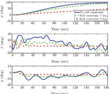
propeller shaft speed is to be constant at 90 rpm, sim-ulations are performed with dierent roll constraints imposed, and the results are summarized in Figure 3. From Figure 3, we can see that, the more the roll constraint is tightened, the less tracking performance is achieved. This is because the large rudder action is not permissible due to the roll constraints. When there is no roll constraint, the vessel reaches the desired heading, but, for roll constraint of 7 deg, the desired heading is not achieved. For roll constraint of 3 deg, the heading error is high, needing more time to converge
Figure 3. Simulation results of the ship response with dierent roll constraints.
to zero. However, since the roll angle of the vessels seriously increase in the presence of wave loads [18], enforcing roll constraints while maneuvering in seaways should be considered.
4.2. Course-changing autopilot
During course-changing maneuvers (path tracking), it is desirable to specify the dynamics of the desired heading instead of using a constant reference signal presented in the course-keeping mode. The amount of change in the heading angle is determined from the desired heading the controller needs to track, which is commanded either by a helmsman/pilot or an autopilot [19].
In the simulations performed in this section, the desired heading response has been commanded by
c= 0:0025t, which makes the ship track a circular
path [20]. The initial state of the vessel is chosen to be x0 = [6ms; 0; 0; 0; 0; 0; 0; 0; 66 rpm; 0]T and it is
assumed that the propeller shaft speed is to be constant at 66 rpm. The roll angle limit is jj 20 deg.
To track the mentioned pilot input, a quadratic cost functional is dened as follows:
J =
tf
Z
0
P ( c)2+ Rc2
dt: (10)
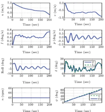
Figure 4 shows the vessel course in the earth-xed coordinate for P = 103 and R = 10. The vessel
starts to move from the origin and track the reference heading.
Figure 5 depicts the states of the ship dynamic model. The motion of the rudder produces drag forces that slow down the vessel during turning. The values of roll and rudder angles do not exceed their limits. The rudder system of the vessel is a rst order system with a one second delay time (Eq. (7)). So there is a little
Figure 4. The vessel course in the earth-xed coordinate for course changing maneuver.
Figure 5. The states of ship dynamic model for course changing maneuver.
dierence between the commanded and actual rudder angles. As seen in Figure 4, the vessel exactly tracks the commanded heading of the helmsman or autopilot system.
5. Conclusion
In this paper, an optimal control approach, addressing the tracking control of underactuated marine surface vessels, is presented. The detailed optimal controller formulation and its transcription to NLP via direct GPM is described. The simulation results for course-keeping and course-changing maneuvers show that GPM can achieve precise tracking control of marine surface vessels, while satisfying the prescribed input and state constraints, without needing to linearize their dynamical models.
References
1. Do, K.D. and Pan, J., Control of Ships and Underwater Vehicles: Design for Underactuated and Nonlinear Marine Systems, Springer (2009).
2. Lefeber, E., Pettersen, K.Y. and Nijmeijer, H. \Track-ing control of an underactuated ship", IEEE Trans-actions on Control Systems Technology, 11, pp. 52-61 (2003).
3. Jiang, Z.P. \Global tracking control of underactuated ships by Lyapunov's direct method", Automatica, 38, pp. 301-309 (2002).
4. Avgouleas, K. \Optimal ship routing", MSc Thesis,
Department of Mechanical Engineering, Massachusetts Institute of Technology, United States, Massachusetts (2008).
5. Li, Z., Sun, J. and Oh, S. \Path following for marine surface vessels with rudder and roll constraints: An MPC approach", in American Control Conference, St. Louis, MO, USA, pp. 3611-3616 (2009).
6. Ghaemi, R. \Robust model based control of con-strained systems", Ph.D. Thesis, The University of Michigan (2010).
7. Cimen, T. and Banks, S.P. \Nonlinear optimal track-ing control with application to super-tankers for au-topilot design", Automatica, 40, pp. 1845-1863 (2004).
8. Betts, J.T. \Survey of numerical methods for trajec-tory optimization", Journal of Guidance, Control, and Dynamics, 21, pp. 193-207 (1998).
9. Benson, D. \A Gauss pseudospectral transcription for optimal control", Ph.D. Thesis, Massachusetts Institute of Technology, United States, Massachusetts (2005).
10. Huntington, G. \Advancement and analysis of a Gauss pseudospectral transcription for optimal control problems", Ph.D. Thesis, Massachusetts Institute of Technology, United States, Massachusetts (2007).
11. Trefethen, L.N., Spectral Methods in Matlab: Society for Industrial and Applied Mathematics (2000).
12. Gill, P.E., Murray, W. and Saunders, M.A. \SNOPT: An SQP algorithm for large-scale constrained opti-mization", SIAM Review, 47, pp. 99-131 (2005).
13. Garg, D., Patterson, M., Hager, W.W., Rao, A.V., Benson, D.A. and Huntington, G.T. \A unied frame-work for the numerical solution of optimal control problems using pseudospectral methods", Automatica, 46, pp. 1843-1851 (2010).
14. Salarieh, H. and Ghorbani, M. \Trajectory optimiza-tion for a high speed planing boat based on gauss pseu-dospectral method", The 2nd International Conference on Control, Instrumentation and Automation (ICCIA 2011), Shiraz University (2011).
15. Fossen, T.I., Guidance and Control of Ocean Vehicles, Wiley (1994).
16. Cimen, T. \On-line nonlinear optimal maneuvering control of large tankers in restricted waterways", The 7th IFAC Conference on Manoeuvring and Control of Marine Craft (MCMC'2006), Lisbon, Portugal (2006).
17. Kirk, D.E., Optimal Control Theory: An Introduction, Dover Publications (2004).
18. Banazadeh, A. and Ghorbani, M.T. \Frequency do-main identication of the Nomoto model to facilitate Kalman lter estimation and PID heading control of a patrol vessel", Ocean Engineering, 72, pp. 344-355 (2013).
19. Cimen, T. \Development and validation of a math-ematical model for control of constrained non-linear
oil tanker motion", Mathematical and Computer Mod-elling of Dynamical Systems, 15, pp. 17-49 (2009).
20. Cheng, J., Yi, J. and Zhao, D. \Design of a sliding mode controller for trajectory tracking problem of marine vessels", IET Control Theory & Applications, 1, pp. 233-237 (2007).
Biographies
Mohammadtaghi Ghorbani was born in Kashan, Iran, in 1987. He received his BS degree in Mechanical Engineering from Kashan University, Kashan, Iran, in
2009, and his MS degree in Mechatronic Engineering in 2012 from Sharif University of Technology, Tehran, Iran. His special elds of interest include optimization and optimal control.
Hassan Salarieh received his BS degree in Mechanical Engineering and Pure Mathematics, in 2002, and MS and PhD degrees in Mechanical Engineering in 2004 and 2008, respectively, from Sharif University of Technology, Tehran, Iran, where he is currently Associate Professor in Mechanical Engineering. His elds of research are dynamical systems, control theory and stochastic systems.