Wave height analysis from 10 years of observations in the
Norwegian Sea
Xiangbo Feng1,2*, M. N. Tsimplis1, G. D. Quartly3 and M. J. Yelland1
(final version submitted to Cont. Shelf. Res. 11/10/13 doi 10.1016/j.csr.2013.10.013 )
Abstract
Large waves pose risks to ships, offshore structures, coastal infrastructure and ecosystems. This paper analyses 10 years of in-‐situ measurements of significant wave height (Hs) and maximum wave height (Hmax) from the ocean weather ship Polarfront in the Norwegian Sea. During the period 2000 to 2009, surface elevation was recorded every 0.59 s during sampling periods of 30 minutes.
The Hmax observations scale linearly with Hs on average. A widely-‐used empirical Weibull distribution is found to estimate average values of Hmax/Hs and Hmax better than a Rayleigh distribution, but tends to underestimate both for all but the smallest waves. In this paper we propose a modified Rayleigh distribution which compensates for the heterogeneity of the observed dataset: the distribution is fitted to the whole dataset and improves the estimate of the largest waves. Over the 10-‐year period, the Weibull distribution approximates the observed Hs and Hmax well, and an exponential function can be used to predict the probability distribution function of the ratio Hmax/Hs. However, the Weibull distribution tends to underestimate the occurrence of extremely large values of Hs and Hmax.
The persistence of Hs and Hmax in winter is also examined. Wave fields with Hs>12 m and
Hmax>16 m do not last longer than 3 hours. Low-‐to-‐moderate wave heights that persist for more than 12 hours dominate the relationship of the wave field with the winter NAO index over 2000-‐2009. In contrast, the inter-‐annual variability of wave fields with Hs>5.5 m or
Hmax>8.5 m and wave fields persisting over ~2.5 days is not associated with the winter NAO index.
1. Introduction
Large ocean waves pose significant risks to ships, offshore structures, coastal infrastructure and coastal ecosystems. The development of offshore installations for oil and gas extraction and for renewable energy exploitation requires knowledge of the wave fields and any potential changes in them. Waves are also important in understanding aspects of ocean dynamics such as surface wind stress, and near-‐surface mixing which in turn affects the air-‐ sea fluxes of gases and heat (Melville and Matusov, 2002). Waves play a role in the mixing and dispersal of pollutants (Giarrussoa et al., 2002) and also contribute to the levels of underwater noise (Leighton, 1994) thus affecting the behavior of many cetaceans.
Most information presently available for wave fields is presented in terms of the significant wave height (Hs). Hs is defined as the average height of the highest one-‐third of the waves,
which in the deep ocean equates to four times the square root of the zeroth moment of the narrow-‐band wave spectrum (Sverdrup and Munk, 1947; Phillips, 1977). Knowledge of the maximum peak-‐to-‐trough wave height (Hmax) is not usually available although these largest waves have the most significant impact on ocean engineering, safety and financial concerns. Lack of data has made it necessary to estimate Hmax from its expected statistical relationship with Hs. Assuming that the statistics of stochastic ocean waves are stationary, Hmax estimates have been made using the Rayleigh distribution (Longuet-‐Higgins, 1952; Sarpkaya and Isaacson, 1981). However, in some cases where Hmax observations did exist, this method has been found to overestimate the largest individual wave heights (Forristall, 1978; Tayfun, 1981; Krogstad, 1985; Massel, 1996; Nerzic and Prevosto, 1997; Mori et al., 2002; Casas-‐Prat
and Holthuijsen, 2010). Some of the discrepancy is known to be due to the effect of the spectral bandwidth, i.e. the gathering of wave components around the peak energy component (Tayfun, 1981; Ochi, 1998; Vandever et al., 2008). The nonlinearity of wave-‐wave interaction has also been found to affect the crest height and trough depth distributions, but not the individual wave height (Tayfun, 1983; Casas-‐Prat and Holthuijsen, 2010). In contrast to observations, recent laboratory experiments and theoretical model studies show that the nonlinearity affects the wave height distributions, and that this effect depends on the state of wave development (Slunyaev and Sergeeva, 2012; Ying and Kaplan, 2012). What has now been confirmed both from theories and measurements is that the nonlinear wave interactions have significant impact on the ratio of the maximum wave height to significant wave height (Hmax/Hs) (Janssen, 2003; Mori and Janssen, 2006).
Forristall (1978) and Gemmrich and Garrett (2011) have shown that the Weibull distribution provides a better estimate of the observed largest wave heights, i.e. those with the lowest probability of being exceeded. Because the parameterization of the Weibull distribution depends on the local sea state, it is not easy to apply in practice. Forristall (1978) suggests an empirical fit to the Weibull distribution based on the number of waves in the observational record. The significant improvement in estimating Hmax was confirmed using clustered or ensemble wave height distributions by Forristall (2005), Casas-‐Prat and Holthuijisen (2010) and Waseda et al. (2011). However, the lack of long-‐term Hmax observations means that neither of the statistical distributions has been fully evaluated in all conditions.
In this paper we investigate Hs, Hmax and the persistence of wave fields using 10 years of 30-‐ minute sea surface elevation records from a Ship-‐Borne Wave Recorder (SBWR) at Ocean Weather Station (OWS) Mike in the Norwegian Sea. We systemically evaluate the capability of the Rayleigh distribution and the corrected method by Forristall (1978) in estimating Hmax/Hs, and the resulting Hmax, against the 30-‐minute records. The long-‐term distributions of wave heights and persistence are also explored.
The paper is structured as follows. The data and methodology are described in Section 2, along with the statistical definitions to be used. A new parameter, "run length", is introduced to describe the persistence of wave fields that exceed given thresholds. Section 3 examines the short-‐term statistics of the observations of Hmax/Hs and Hmax, and how they vary from theoretical predictions. The long-‐term (10-‐year) distributions of Hs, Hmax, Hmax/Hs and run length are then discussed. In Section 4, the temporal variability of the wave field is correlated with the winter NAO index to show which aspects of the winter wave climate are affected by the large-‐scale changes in the overall sea level pressure field, as opposed to being caused by individual storms. Our conclusions are given in Section 5.
2. Data and methodology
2.1. Ship-‐Borne Wave Recorder (SBWR) data
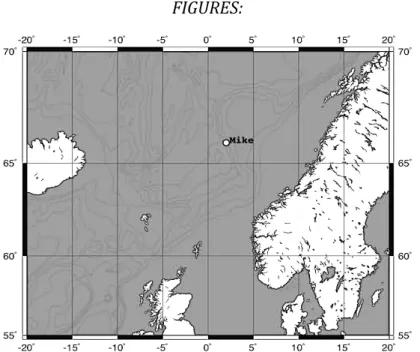
Ocean Weather Station Mike (OWS Mike, 66˚N, 2˚E in the Norwegian Sea, Figure 1) was occupied by an ocean weather ship for more than 60 years until the ship Polarfront was withdrawn at the end of 2009. The sea surface elevation was measured by a Ship-‐Borne Wave Recorder (SBWR) and wave height data from this system are available from 1980 to the end of 2009.
The SBWR was developed by the UK National Institute of Oceanography (later to become part of the National Oceanography Centre) in the 1950s and is considered a very reliable system (Graham et al., 1978; Holliday, et al., 2006). The SBWR uses the surface-‐following properties of the platform to capture the longer wavelength waves, and pressure sensors mounted in the hull to measure shorter wavelength waves. Polarfront was a relatively small ship (49 m length) and spent most of the time drifting beam-‐on to the waves, but the response of the ship to the waves tends to flatten the measurement of the wave crests and sharpen the troughs (Magnusson, et al., 1999). A short, 30-‐hour comparison between observations obtained by the SBWR on Polarfront and those from a wave-‐rider buoy showed good agreement, with the SBWR underestimating Hs by 0.4 m on average (Clayson, 1997).
From 1980 until the end of 1999, only the integrated wave parameters (e.g. Hs and average period) were recorded by the SBWR system: these have been analysed briefly elsewhere (Yelland et al., 2009). However, for the last 10 years of operation (2000-‐2009, the period investigated in this paper) the SBWR system also recorded the sea surface elevation every 0.59 s for the 30-‐minute sampling periods, with sampling occurring once every 90 minutes before the 250th day of 2004, and once every 45 minutes thereafter.
The height of an individual wave is defined as the vertical distance between a wave trough and the following wave crest. For each 30-‐minute record, the highest individual wave is identified as Hmax, and Hs is calculated from four times the square root of the zeroth-‐order moment of the wave frequency spectrum within 0.02-‐0.85 Hz.
2.2 Data quality
The reliability of the measurement of individual waves is of significant importance in the analysis of extreme waves. Significant uncertainty can be introduced in to the sea surface elevation measurement depending on: the type of platform used; the way the platform interacts with the waves; the type of measuring instrument; the instrument's ability to measure very steep changes of the sea surface e.g. waves that are about to break; the relationship between a point measurement and the multi-‐dimensional wave profile. These issues are discussed in detail by Liu and MacHutchon (2006), Christou and Ewans, (2011a,b) and Forristall, (2005) and affect all in-‐situ measurements to some extent.
The performance of SBWRs mounted on light vessels and other ships has been validated against data from wave buoys in terms of Hs and spectrum by Graham et al [1978], Crisp
[1987] and Pitt [1991]. In the case of Polarfront the only validation was the 30-‐hour comparison with a wave buoy made by Clayson (1997). The lack of validation comparisons is a general problem for wave measurements made from numerous platforms and instruments (Christou and Ewans, 2011a). In the case of the SBWR on Polarfront we cannot exclude the possibility of systematic biases such as the 0.4 m underestimate as found by Clayson (1997). In normal operations, Polarfront was allowed to drift without engine propulsion, provided it remained within a 32km radius around the location known as OWS Mike. Once outside this radius the ship steamed slowly back to station with a speed of up to 5m/s at most. The ship stayed on station all year round, except for 3 days out of every 28 when it returned to port. These days on passage to port and back were not included in the analysis: this removed about 11 % of the available 30-‐minute wave records. Further quality control was applied by examining various wave parameters (e.g. Hmax, Hmax/Hs, maximum wave period) to identify extreme and/or potentially un-‐realistic values. All of these records were then checked by visually examining the wave trace over the whole of the 30-‐minute record. A total of 524 physically unrealistic wave traces were identified in this fashion: most of these events were associated with unusually large changes in ship speed and direction. It should be noted that when an unrealistic trace was detected, the entire 30-‐minute record was removed from the analysis.
In total, the quality control led to a rejection of 10,678 out of 81,888 (13%) thirty-‐minute wave records. This procedure left 17,389,559 individual waves in a total of 71,210 records obtained over 2,915 days between 2000 and 2009.
2.3. Statistical distributions of waves
Longuet-‐Higgins (1952) suggests that, in the deep ocean, individual waves with a narrow-‐ band wave spectrum follow a Rayleigh distribution. Thus, for a given observational period, the ratio of observed maximum wave height Hmax and the average height of the highest one-‐third of the waves, H1/3, can be theoretically presented as a function of N, the number of individual crest-‐to-‐trough waves in the record (Sarpkaya and Isaacson, 1981):
max 1/ 3
ln 1.42
H N
H = (1)
wave height Hs, defined as four times the square root of the zero-‐order moment of the spectrum. Hs (rather than H1/3) are usually recorded from in-‐situ measurements. The probable maximum wave height, Hmax* , is then related to Hs through the equation:
Hmax*
Hs =
lnN
1.42 (2)
Therefore, the probable maximum wave height Hmax* in a given period can be calculated from the observed Hs and N using Eq. (2).
The theoretical exceedence probability function F(H) of the wave height H, derived from a 2-‐ parameter Weibull distribution, is given by Holthuijsen, (2007) as:
( , , ) exp[ ( ) ]H
F H β α β
α
= − (3)
where α is a scale parameter and β denotes a slope parameter.
In order to fit Eq. (3) to the wave measurements H (in terms of Hs or Hmax) from the 10 years of observations, the observed wave heights are first sorted into ascending order H(j)
(j=1,2,3,…,M). Let M be the total number of waves involved, and let 1/M be the probability density of each wave event. The exceedence probability, F, of waves over a height of H(j) is then estimated as:
F(H(j))=1-‐j/(M+1) , (j=1,2,3,…,M) (4)
The wave height H(j) at specific exceedance probability F(H(j)) can be inverted from Eq. (4).
2.4. Persistence and run length
We develop a measure of the time during which Hs or Hmax remains above a specific threshold. We define the persistence T as the period during which a particular characteristic H (in terms of either Hs or Hmax) of the wave field continuously exceeds a threshold value Hc. We further define run length, L, which reflects the total amount of time during an extended period (for example December to March) over which a) the wave field parameter H exceeds the threshold
1
( c, c) ni ( )
L H H T T T i
=
> > =
∑
(5)Thus persistence measures how long the wave field exceeds the height threshold during an individual storm, whereas run length is a measure of the total time during which the wave field stays over a certain persistence threshold.
Finally, dividing run length L by the total persistence T (i.e. Tc set to zero) provides F, the exceedance percentage of run length, for a given Hc. Physically, F gives the probability of waves exceeding a given height Hc for different persistence Tc.
An example is given in Figure 2 for a run length L(H>5 m, T>12 hours). For clarity we use a short observational period of only 240 hours (rather than the four winter months for example). The wave height threshold Hc of 5 m is exceeded for eight periods denoted as T(1, 2, …, 8), the total duration of which is 127 hours. Four of the periods persist for longer than the threshold Tc of 12 hours: T(1, 2, 4, 7)=16, 14, 50 and 28 hours. Thus, the run length L(H>5 m, T>12 hours)=
∑
i=1,2,4,7T i( ) =108 hours. The exceedance percentage of run length is thencalculated as F(H>5 m, T>12 hours)=
∑
i=1,2,4,7T i( ) /∑
i8=1T i( ) =108/127=85%. This tells us thatwhen the wave height threshold of 5 m is exceeded the wave field will exceed the threshold for 12 hours or more, for 85 % of the time. In other words, when the wave height threshold is exceeded, 85% of such wave fields will persist 12 hours or more.
3. Results
3.1. Short-‐term statistics of Hmax/Hs
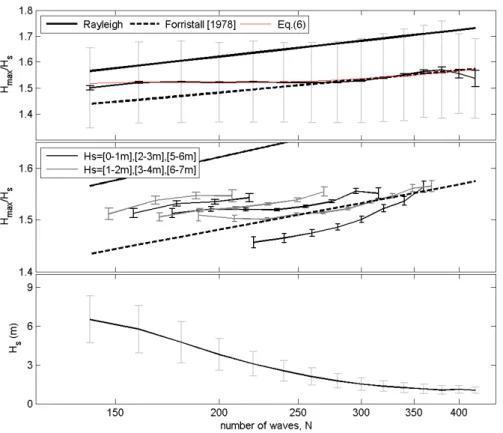
Eq. (1) suggests that, assuming a Rayleigh distribution, the value of Hmax/Hs will vary linearly with (ln N)0.5. However, Figure 3 (upper) shows that the 30-‐minute in-‐situ observations do not behave in this way, and the observations are significantly lower than those predicted from the Rayleigh distribution. For the average value of N≈250, the theoretical value of Hmax/Hs is 1.65 while the observed value is 1.53. Thus, the Rayleigh distribution overestimates Hmax/Hs by 8% on average.
Forristall (1978) suggests an empirical correction coefficient of between 0.90 and 0.96 (depending on N) to bring the Rayleigh estimates of Hmax/Hs into better agreement with those from a Weibull distribution (Figure 3 upper). At low N the Forristall values underestimate the
observations, by about 3% for N≈150. The mean value of Hmax/Hs from Forristall (1978) is 1.50, 2% lower than the observed mean value of 1.53. Therefore, the empirical fitted Weibull distribution from Forristall (1978) gives a reasonable estimate for the mean value of Hmax/Hs. The observed individual values of Hmax/Hs are very widely scattered as shown by the faint error bars in the upper panel of Figure 3. About 35% of the observations have ratios of
Hmax/Hs that do not lie in the range 1.4 to 1.75, i.e. the maximum range predicted by the two statistical methods. In addition 0.9% of records (636/71210) have Hmax/Hs values exceeding 2.0. Such waves are defined as freak waves (Mori and Janssen, 2006). The standard deviation of the estimated Hmax/Hs from the observed values is 0.16 for both methods. Thus in observations the ratio Hmax/Hs is centered on 1.53 but the individual values are very widely distributed around the mean and are not dominated by N as expected.
Figure 3 (upper) shows that, in the mean, the observed relationship of Hmax/Hs to N does not agree with the linear relationships suggested by the Rayleigh distribution and the Forristall correction either. The black error bars on Figure 3 (upper) represent the standard error, rather than the standard deviation. Figure 3 (lower) shows that Hs decreases with increasing N, as expected: here the faint error bars indicate the standard deviation of the data. The observed mean Hmax/Hs has no dependence on N for N between 170 and 300 waves per 30-‐ minute period. For N between 300 and 380, corresponding to Hs values of less than 1.5 m, the observations indicate a trend with N (similar to that shown in theory) and also with Hs. The reduction in Hmax/Hs for N > 380 (where the mean Hs is only 1 m), is probably not significant in this dataset. The disagreement between observations and theory could be caused, as one reviewer suggested, by the inhomogeneous character of the sea states in our dataset. This suggestion is supported by the studies of Stansell (2004, 2005) who used 33 days of data recorded during 14 storms in the North Sea to show qualitatively that the Hmax/Hs ratio is independent of the sea state when examining the dataset as a whole, but weakly dependent on sea state when a limited range of sea state was used. However, the Stansell dataset was too small to determine a clear trend. To investigate this, our 10-‐year dataset was split into subsets according to Hs (i.e. Hs between 0 to 1 m, 1 to 2 m etc). The Hmax/Hs to N relationship for each subset is shown separately in the middle panel of Figure 3 (for clarity not all subsets are shown, i.e. the 4-‐5 m range is omitted, as are data with Hs over 7 m). It can be seen that each subset shows an increase in the Hmax/Hs ratio with increasing N, with a slope that is similar to that expected from theory. For large N (300 to 380) only the two smallest Hs subsets (0 to 1 and 1 to 2 m) are present which explains the trend seen in the upper plot. For N less than
300, it can be seen that there is a much greater range of Hs classes for a given value of N: this explains the lack of any trend in the upper panel, i.e. the inhomogeneity of sea states masks the theoretical dependence of Hmax/Hs on N.
It is interesting to note that for a given constant N, the ratio of Hmax/Hs increases with increasing Hs. In the middle panel of Figure 3, the subset of data where Hs is about 1.5 m on average (lowest grey line) fits the line representing the Forristall relationship well across a wide range of N. This observation was used to develop the following empirical fit by modifying Eq. (1) as follows:
max ln 1.7( 1.5)
1.555 100
s s
H N H
H
−
= + (6)
Here the denominator in the first term on the right hand side has been increased compared to that in Eq. (1) to allow for the difference between our mean Hmax/Hs and that predicted from the Rayleigh relationship. The second term evaluates to zero for an Hs of 1.5 m, and increases with increasing Hs. The other constants in the second term were tuned to produce the best fit to the mean of the observed Hmax/Hs values shown in the upper panel of Figure 3. Applying this new model to the whole 10-‐year dataset results in the mean predicted Hmax/Hs ratios shown by the red line in the upper panel of Figure (3). It can be seen that Eq. (6) models the observed mean values very well. However, the right hand term explains less than 1% of the variance in the observed Hmax/Hs ratios since the scatter in the individual observed values is very large (grey error bars, upper panel).
Janssen (2003) argues that the nonlinearity of wave interactions plays an important role in producing extreme values of Hmax/Hs. Mori and Janssen (2006) showed that the occurrence of high values of Hmax/Hs can be related to a) the number of waves in the record and b) the kurtosis of the sea surface elevation distribution. The kurtosis is the normalized fourth-‐order moment of surface elevation η, i.e. <η4>/<η2>2. Kurtosis reflects the nonlinearity of wave
processes, and a kurtosis value of 3 indicates a normal distribution. A kurtosis value >3 (or <3) represents distributions that are more "peaked" (or "flat") compared to a normal distribution. Studies made in coastal waters with limited data records (a few days or months), have confirmed a link between Hmax/Hs and kurtosis (Mori and Janssen, 2006; Liu et al., 2009;
Cherneva et al., 2011).
The observed ratio Hmax/Hs is found to have a clear linear relationship with kurtosis (but generally not with N as discussed above) as shown in Figure 4. The linear regression of
Hmax/Hs with kurtosis is:
Hmax/Hs=(0.49±0.01)*kurtosis (7)
The correlation of the kurtosis and Hmax/Hs is 0.55, implying that kurtosis explains nearly 30% of the variance in Hmax/Hs. We thus confirm the Mori and Janssen (2006) analysis that the ratio of Hmax/Hs is related to kurtosis.
This relationship permits the prediction of Hmax/Hs assuming that kurtosis is known. Janssen (2003) suggests that the kurtosis theoretically depends on the Benjamin–Feir Instability (BFI), i.e. a ratio of the effects of nonlinearity and wave dispersion. Additionally, wave kinetic models (Annenkov and Shrira, 2009) indicate that a freshening sea state will lead to a period of consistently larger values for the kurtosis, i.e. peakier waves. However, our in-‐situ observations show no significant correlation of BFI (calculated following the method of
Janssen (2003)) with kurtosis or with Hmax/Hs, indicating that the attempt to predict Hmax/Hs using spectral geometry failed. We also find that the value of kurtosis appears to have negligible persistence, i.e. poor correlation between succeeding records 45 minutes apart. That is contrary to expectations from the theoretical models (Annenkov and Shrira, 2009) that kurtosis would change accordingly and persist for a certain period when wind fields are adjusted. Our results imply that a time series of past kurtosis values will not enable us to improve short-‐term prediction of the ratio Hmax/Hs.
3.2. Short-‐term statistics of Hmax
The probable maximum wave height, Hmax* , is calculated from the theoretical ratio of Hmax/Hs and Hs. The blue, red and black circles in Figure 5 show the scattered distributions of the calculated Hmax* , using the theoretical ratios of Hmax/Hs derived from the Rayleigh distribution (Hmax/Hs=(ln N)0.5/1.42), the corrected method by Forristall (1978) and Eq. (6), against Hs. The calculated Hmax* can be approximated as a linear function of Hs, with
* max
H =(1.65±0.03)*Hs
from the Rayleigh distribution, Hmax* =(1.50±0.02)*Hs from the Forristall method, and *
max
H =(1.53±0.02)*Hs from Eq. (6). For all the individual 30-‐minute observations (grey dots in
Figure 5), the linear regression is Hmax=(1.53±0.16)*Hs. The observations are much more widely scatted than those from the statistical methods. Eq. (6) was tuned to the observed values, so the agreement in slope between the Eq. (6) relationship and that in the observations is to be expected.
The average ratio of Hmax* from the Rayleigh distribution to the observed Hmax is 1.09, indicating that that formula overestimates the maximum wave height by 9%. Using the corrected method by Forristall (1978) reduces this ratio to 0.99, a big improvement from the Rayleigh. Our empirical approach of Eq. (6) produces an average ratio of 1.01. No method reproduces the large scatter seen in the observations.
The performance of the corrected method by Forristall (1978) is found to vary with Hs. For
Hs<6 m, the average ratio between Hmax* and observed Hmax is 1.0, while for Hs>6 m, the average ratio is 0.96. For the highest sea states observed (Hs>10 m ) the Forristall estimate is still low by 4.5% on average (red circles in Figure 5). Thus, the corrected method by Forristall (1978) generally underestimates the maximum wave height of the largest waves, whereas the Rayleigh method and Eq. (6) both predict these waves reasonably well.
The discrepancy between estimated Hmax* and observed Hmax is largely due to the estimation of Hmax/Hs. For example, when the Rayleigh method overestimates Hmax/Hs by 8% on average (see Section 3.1), the resulting Hmax* is 9% higher than observed Hmax. When Hmax/Hs is underestimted by 2% using the corrected method from Forristall (1978), the resulting Hmax* is 1% low. Similarly, when Eq. (6) is used, the improved estimation of Hmax/Hs results in reasonable Hmax* even for highest sea states.
The effect of spectral bandwidth on the estimate of Hs is also expected to contribute to the discrepancy in the Hmax* estimates. For a narrow-‐band spectrum, Hs estimated from the spectrum equates to the average height of the highest one-‐third of the waves, H1/3, as calculated from the wave height distribution (Phillips, 1977). However, when the spectral bandwidth increases, Hs tends to overestimate H1/3 (Tayfun, 1981; Ochi, 1998; Vandever et al., 2008). This overestimate of H1/3 will in turn contribute to the discrepancy in Hmax* from any of the methods.
In conclusion, on average the observed Hmax is a linear function of Hs but the individual values show a fairly large degree of scatter about the mean relationship. The corrected method by
Forristall (1978) models Hmax well on average but tends to underestimate Hmax under high seas. Our empirically fitted method gives improved estimates both on average and for the high sea states.
3.3. Long-‐term statistics of Hs, Hmax and Hmax/Hs
The long-‐term observations of Hs and Hmax over 2000-‐2009 follow a Weibull distribution (see Eq. (3)) with slope parameters of 2.7 and 4.3 respectively and the same scale parameter of 1.5 for both (Figure 6). The Weibull distribution performs well for non-‐extreme wave heights, i.e. those that are exceeded more frequently than 0.08%. This confirms the conclusion of
Holthuijsen (2007) that the Weilbull distribution can model the long-‐term distribution of Hs well.
However, for the largest 0.08% of waves, when Hs is over 12 m and Hmax is over 16 m, the observed wave heights are higher than those predicted by the Weibull distribution. The discrepancy increases with increasing wave height. For example, the highest Hs observed is 15.18 m and the highest Hmax is 25.57 m (both occurred on November 11th 2001), but the Weibull distribution predicts the wave heights of only 13.5 m and 21.5 m respectively. Our results therefore show that the highest 0.08% of waves are underestimated by the Weibull distribution by up to 11% for Hs and 16% for Hmax.
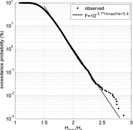
The observed ratio of Hmax/Hs is shown in Figure 7. We tried various distributions to describe the observed dataset and found that the exponential function F=10-‐3.7*Hmax/Hs+5.4 models Hmax/Hs ratios reasonably well for values between 1.6 and 2.4, but tends to underestimate the ratio for Hmax/Hs>2.4. Khadif et al. (2009) have proposed on theoretical grounds that the Benjamin-‐Feir Instability may lead to high ratios of Hmax/Hs. Our observations show an increase in the occurrence of ratios greater than 2.4 which may support this suggestion. However there are only 12 observations in this range so no firm conclusions can be drawn. In the 10-‐year dataset available to us, 636 individual waves are identified as freak waves according to the definition of Mori and Janssen (2006), i.e. individual waves higher than two times the corresponding Hs. The occurrence of freak waves is 3.7*10-‐3% of the total number of waves recorded in our 10-‐year dataset. This is similar to that of ~3*10-‐3% found from a comprehensive dataset in the North Sea (Christou and Ewans, 2011b), but much less than the Rayleigh prediction of 3.1*10-‐2% (Eq. (1)). Of the 30-‐minute records in our dataset, 0.89% contained events where Hmax/Hs>2. This is similar to the 0.77% occurrence found using 20-‐ minute records obtained in the North Sea (Christou and Ewans, 2011a), but much less than the 2.1% found on the Norwegian continental shelf, also from 20-‐minute records (Waseda et al., 2011).
3.4. Long-‐term statistics of run length
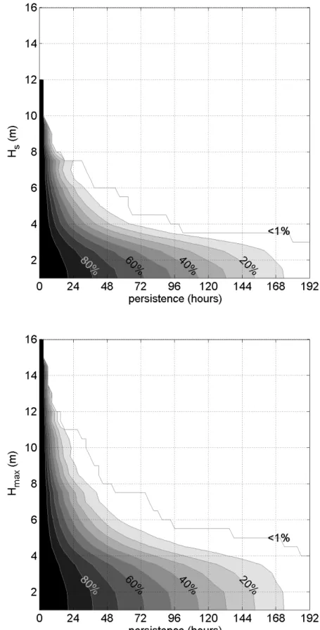
Here we consider winter run lengths for wave heights up to 16 m and persistence of up to 192 hours over the observational duration of winter (December-‐March). The upper panel of Figure 8 shows the average (over the 10 winters) of exceedance percentage of run length, F, for values of Hs as a function of persistence T.
The highest seas last for only very short periods: the wave fields with Hs>12 m do not last more than 3 hours. For F=50% the figure represents the winter persistence of wave heights with median occurrence. For example, for 50% of the cases where Hs>6 m the significant wave height will continuously exceed this height for 12 hours. In less than 1% of the cases, Hs will continuously exceed 6 m for more than 54 hours. Similarly, for the wave fields of Hs>4 m, there is a 50% chance that Hs>4 m will persist over 24 hours and less than 1% chance that Hs >4 m will persist over 96 hours.
The upper panel of Figure 8 also demonstrates that the persistence of the wave field decreases with increasing wave height, as expected. The wave fields with Hs>12 m last only a few hours, whereas those with Hs>3 m can last in excess of 192 hours. The rate of the persistence decrease (i.e. the slope of the F values with persistence) is greater for low seas than for high seas. For instance, the persistence for F=50% reduces by about 70 hours when
Hs increases from 1 m to 4 m and by 15 hours when Hs increase from 4 m to 7 m.
Persistence of Hmax behaves similarly to that of Hs, apart from a more rapid decrease at high values of Hmax (lower panel of Figure 8). This suggests that the persistence of Hmax over different observational periods is basically dominated by the persistence of mean wave conditions.
4. The temporal variability of the wave field
Over the period 2000-‐2009 the trends in annual mean Hs and Hmax are 2.03±4.78 and 2.61±7.28 cm/year respectively. Neither of these trends are statistically significant at the 95% level. This result contrasts with the results for the period 1980-‐1999 during which a significant increase in annual mean Hs of 3.86±1.67 cm/year has been observed by Yelland et
al. (2009) who also used SBWR data from the Polarfront (note that Hmax values were not available prior to 2000).
100 to 500. Since winter wave conditions tend to have longer period waves (and thus smaller values of N for 30-‐min sampling periods) a seasonal variability in Hmax/Hs might be expected. However, such seasonality is not apparent in these observations; nor do we find the annual mean ratio to show a dependence on annual mean wave height. This is because the observed ratio of Hmax/Hs is not significantly influenced by the number of waves in the records, nor by the mean wave heights.
The North Atlantic Oscillation (NAO) is a major large-‐scale atmospheric pattern in this region and is particularly important in winter (Hurrell, 1995; Hurrell and Van Loon, 1997; Osborn et al., 1999). The status of the NAO is represented by the NAO index, determined from the non-‐ dimensional sea level pressure difference between the Icelandic Low and the Azores High. The mean Hs variability in the North Atlantic was found to be associated with the NAO index over the 20th century (Bacon and Carter, 1993; Kushnir et al., 1997; Bauer, 2001; Wang and Swail, 2001, 2002; Woolf et al., 2002; Tsimplis et al., 2005; Wolf and Woolf, 2006; Bertin et al., 2013).
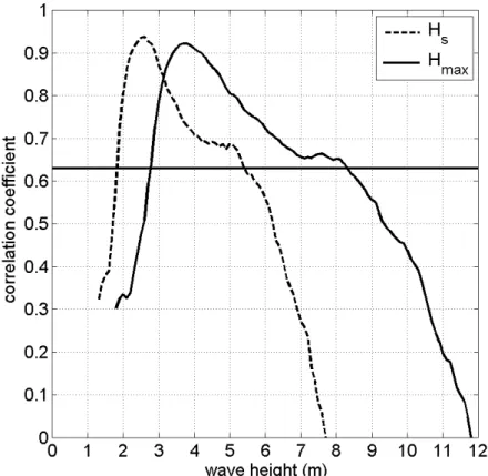
Dodet et al. (2010) showed that in numerical model hindcasts the association also exists for other integrated wave parameters (e.g. wave period and dominant wave direction). These hindcasts suggest that the influence of the NAO extends to the largest 1% of Hs in the North Atlantic during winter (Wang and Swail, 2001, 2002). Izaguirre et al. (2010) used satellite Hs data to show that the extreme wave climate off the Atlantic coast of the Iberian peninsula is also significantly associated with the NAO. In this paper, we assess the impact of the NAO on the temporal variability of the wave fields using the recent in-‐situ observations at OWS Mike. We first consider the observed Hs and Hmax in winter (December-‐March) and how these correlate with the winter NAO index. Time series of the station-‐based NAO index over 2000-‐ 2009 are obtained from the Climate Analysis Section, NCAR, Boulder, USA (http://climatedataguide.ucar.edu). The average value of the NAO index in the boreal winter (December to March) is termed the winter NAO index here. For each given threshold of wave heights, the analysis produces 10 independent values of corresponding occurrences (i.e. one independent measure per season), hence the correlation between the two factors must have a coefficient r exceeding 0.63 to be significant at the 95% level.
The correlation coefficients between the winter NAO index and the exceedance probabilities of specific wave heights are shown in Figure 9. Feng et al. (2013, submitted) showed that the mean wave heights are significantly correlated with the NAO index (r=0.69 and 0.70 for Hs and Hmax). Figure 9 shows that the correlation varies with wave height. For small wave heights (Hs<1.9m, and Hmax<2.8 m), there are very little variations in their annual probabilities
(usually more than 98%), and no statistically significant correlations with the NAO are identified. Wave fields with Hs of 2.5 m and Hmax of 3.5 m are the most highly correlated with the NAO index. However, for wave fields with the largest waves, i.e. Hs>5.5m and Hmax>8.5m, again no significant correlations are found. The lack of correlation between the large waves and the NAO index could be due to these waves being driven by local mesoscale or synoptic weather systems (Reistad et al., 2011) which are not represented by the NAO index in this region (Rogers, 1997). The relationship of the wave heights at OWS Mike with the NAO index has been discussed in detail by Feng et al. (2013, submitted) who found that the correlation with the NAO index was highest for the most frequently-‐encountered (75th percentile) wave heights.
Next we examine the relationship between the persistence of the wave field with the winter NAO index. The correlation of the winter NAO index with the annual exceedance percentage of winter run length, F, for given wave heights (Hs and Hmax) and persistence is shown in Figure 10. The correlation of wave fields with the shortest persistence (3 hours) generally confirms the results in Figure 9. Note that all the significant correlations are found for F in the 50-‐90% range (cf. Figure 8), i.e. for conditions that occur frequently. The correlations are significant for wave fields with an Hs value between 1.5 m and 4.5 m, and an Hmax value between 2 m and 6 m. The highest correlations are found for Hs>2.5 m lasting for more than 12 hours, and for
Hmax>4 m lasting for more than 12 or 30 hours (black areas in Figure 10). However, for wave fields with Hs>4.5 m or Hmax>6 m F is not significantly correlated with the winter NAO index. Figure 10 also indicates that long-‐lived wave fields i.e. those that persist for more than 54 hours for Hs or 63 hours for Hmax, are not associated with the NAO index.
In summary, we confirm that the winter NAO index is associated with the inter-‐annual variability of the low-‐to-‐moderate Hs, and Hmax values, and the persistence of such wave
heights. In contrast, no statistically significant relationship with the NAO index is found for wave fields with the largest waves (Hs>5.5 m or Hmax>8.5 m) or for the wave fields with persistence over ~2.5 days.
5. Conclusions
Ten years of 30-‐minute measurements from a SBWR at OWS Mike over the period 2000-‐2009 were used to analyze the statistics of the wave field in the Norwegian Sea. The Hmax observations have a broad distribution that scales linearly with Hs. The Rayleigh distribution
was found to overestimate Hmax by 9% on average, mainly due to the overestimation of
Hmax/Hs by 8%. The empirical fitted Weibull distribution from Forristall (1978) matches the data better, underestimating Hmax by only 1% on average. However, this method tends to underestimate Hmax for high sea states.
The mean ratio of Hmax/Hs was found to have a linear relation with (ln N)0.5, as theoretically expected, but only for subsets of data with a very small range of Hs values. The relationship is not apparent when the whole dataset is used, since the dataset is heterogeneous and contains a wide range of Hs.. Thus for the whole dataset, the ratio of Hmax/Hs does not have any clear link with N, Hs or seasonality. We introduced an empirical formula to account for the heterogeneity of the dataset: this improved the estimate of the mean Hmax/Hs in terms of N, but only explained less than1% of the variance in the individual data.
In contrast, we found that the Hmax/Hs ratio has a clear linear relationship to kurtosis, which explains 30% of the variance in the individual data. No relationship of Hmax/Hs with the Benjamin-‐Feir index or sea state development was found. An exponential function of 10-‐ 3.7*Hmax/Hs + 5.4 models the occurrence of the ratio of Hmax/Hs reasonably well for values greater than 1.53. Out of a total of 71,210 thirty minute records, 636 contained freak wave events where Hmax/Hs>2.0, i.e. 0.9% of the records from the 10 years.
The vast majority of the observational distribution of Hs and Hmax (i.e. those exceeded more than 0.08% of the time over the 10 years) is approximated well by the Weibull distribution with a scale parameter of 1.5. However the wave heights with the lowest probability of occurrence, i.e. the largest 0.08% of waves, are underestimated by the Weibull distribution. Hmax and Hs are both characteristics of the wave field and both tend to increase in a coherent manner for stronger winds or for longer durations of a consistent wind. However, our results confirmed that the Hmax records in the wave distribution over a short period are not fully determined by the mean conditions (N and Hs) but are also happening randomly to some extent. As Hmax is the pertinent parameter for describing ocean risk and dynamics, we suggest that more measurements of Hmax in conjunction with Hs are needed to better understand how behaviors of the two parameters differ.
A new parameter called run length was defined and analysed. Empirical estimates of the periods over which wave heights exceed specific thresholds and last longer than a given persistence threshold were produced. We confirmed that the persistence of wave fields decreases with increasing wave height. Wave fields with Hs in excess of 12 m and Hmax in
excess of 16 m did not last longer than 3 hours.
Over the period 2000-‐2009 neither Hs nor Hmax at OWS Mike show a significant trend, but both do show a dependence on the NAO index. The relationship of the wave fields with the NAO index over 2000-‐2009 was found to be dominated by the association of the winter NAO index with the low-‐to-‐moderate wave heights persisting over ~12 hours. However, the inter-‐annual variability of wave fields with Hs>5.5 m or Hmax>8.5 m and wave fields persisting over ~2.5 days is not associated with the winter NAO index.
Acknowledgements
This research is funded by Lloyd's Register Foundation, which supports the advancement of engineering-‐related education, and funds research and development that enhances safety of life at sea, on land and in the air. Thanks to Knut Iden of the Norwegian Meteorological Institute, DNMI, for supplying the wave measurements, and the reviewers who gave us very useful comments.
References
Annenkov, S.Y., Shrira, V.I., 2009. Evolution of kurtosis for wind waves. Geophysical Research Letters 36, L13603. Bacon, S., Carter, D.J.T., 1993. A connection between mean wave height and atmospheric pressure gradient in the
North Atlantic. International Journal of Climatology 13, 423–436.
Bauer, E., 2001. Interannual changes of the ocean wave variability in the North Atlantic and in the North Sea. Climate Research 18, 63-69.
Bertin, X., Prouteau, E., Letetrel, C., 2013. A significant increase in wave height in the North Atlantic Ocean over the 20th century. Global and Planetary Change 106, 77-83.
Casas-Prat, M., Holthuijsen, L.H., 2010. Short-term statistics of waves observed in deep water. Journal of Geophysical Research 115, C09024.
Cherneva, Z., Soares, C.G., Petrova, P., 2011. Distribution of Wave Height Maxima in Storm Sea States. Journal of Offshore Mechanics and Arctic Engineering 133(4), 041601.
Christou, M., Ewans, K., 2011a. Examining a Comprehensive Dataset Containing Thousands of Freak Wave Events: Part 1--Description of the Data and Quality Control Procedure. In Proc. 30th Int. Conf. Offshore Mechanics and Arctic Eng.(OMAE), Rotterdam, the Netherlands, OMAE2011-50168.
Christou, M., Ewans, K., 2011b. Examining a Comprehensive Dataset Containing Thousands of Freak Wave Events: Part 2--Analysis and Findings. In Proc. 30th Int. Conf. Offshore Mechanics and Arctic Eng.(OMAE), Rotterdam, the Netherlands, OMAE2011-50169.
Clayson, C.A., 1997. Intercomparison between a WS Ocean Systems Ltd. Mk IV shipborne wave recorder (SWR) and a Datawell Waverider (WR) deployed from DNMI ship Polarfront during March-April 1997. Southampton
Oceanography Centre, Southampton, UK, 26pp. (Unpublished report)
Crisp, G.N., 1987. An experimental comparison of a shipborne wave recorder and a waverider buoy conducted at the Channel Lightvessel. Wormley, UK, Institute of Oceanographic Sciences, 181pp. (Institute of Oceanographic Sciences Report, (235) ).
Dodet, G., Bertin, X., Taborda, R., 2010. Wave climate variability in the North-East Atlantic Ocean over the last six decades. Ocean modelling 31(3), 120-131.
Feng, X, Tsimplis, M.N., Yelland, M.J., Quartly, G.D., 2013. Changes in significant and maximum wave heights at Ocean Weather Station Mike in the Norwegian Sea. Global and Planetary Change, submitted.
Forristall, G.Z., 1978. On the statistical distribution of wave heights in a storm. Journal of Geophysical Research 80, 2353–2358.
Forristall, G.Z., 2005. Understanding rogue waves: Are new physics really necessary. In Rogue Waves: Proc. 14th ‘Aha Huliko’a Hawaiian Winter Workshop, pp29-35.
Gemmrich, J., Garrett, C., 2011. Dynamical and statistical explanations of observed occurrence rates of rogue waves. Natural Hazards and Earth System Sciences 11, 1437–1446.
Giarrusso, C. C., Pugliese Carratelli, E., Spulsi, G., 2001. On the effects of wave drift on the dispersion of floating pollutants. Ocean engineering 28(10), 1339-1348.
Graham, C., Verboom, G., Shaw C.J., 1978. Comparison of shipborne wave recorder and waverider buoy data used to generate design and operational planning criteria. Proceedings 16th International coastal Engineering Conference, Hamburg, Am. Soc. Cir. Eng., New York, N.Y., p97-113.
Hemer, M. A., Fan, Y., Mori, N., Semedo, A., Wang, X.L., 2013. Projected changes in wave climate from a multi-model ensemble. Nature Climate Change 3, 471-476.
Holliday, N.P., Yelland, M.J., Pascal, R., Swail, V.R., Taylor, P.K., Griffiths, C.R., Kent, E., 2006. Were extreme waves in the Rockall Trough the largest ever recorded? Geophysical Research Letters33, L05613.
Holthuijsen, L.H., 2007. Waves in oceanic and coastal waters, Chapter 4 - Statistics, Cambridge University Press, ISBN 0-521-86028-8, p56-105.
Hurrell J.W., Van Loon, H., 1997. Decadal variations in climate associated with the north Atlantic Oscillation. Climate Change 36, 301 – 326.
Hurrell, J.W., 1995. Decadal trends in the North Atlantic Oscillation: Regional temperatures and precipitation. Science 269, 676–679.
Izaguirre, C., Mendez, F.J., Menendez, M., Luceño, A., Losada, I.J., 2010. Extreme wave climate variability in southern Europe using satellite data. Journal of Geophysical Research 115(C4), C04009.
Janssen, P.A.E.M., 2003. Nonlinear Four-Wave Interactions and Freak Waves. Journal of Physical Oceanography 33, 863–884.
Kharif, C., Pelinovsky, E., Slunyaev, A., 2009. Rogue Waves in the Ocean. Springer Berlin Heidelberg. Krogstad, H.E., 1985. Height and period distributions of extreme waves. Applied Ocean Research 7, 158–165. Kushnir, Y., Cardone, V.J., Greenwood, J.G., Cane, M.A., 1997. The recent increase in North Atlantic wave heights.
Journal of Climate 10, 2107–2113.
Leighton T.G., 1997. The Acoustic Bubble (Vol. 10). Academic Press.
Liu, P., Chen, H., Doong, D., Kao, C., Hsu, Y., 2009. Freak waves during Typhoon Krosa. Annales Geophysicae 27, 2633–2642.
Liu, P.C., MacHutchon, K.R., 2006. Are there different kinds of rogue waves? In: Proc. 25th Int. Conf. OMAE 2006, Hamburg, Germany, OMAE2006-92619;
Longuet-Higgins M.S., 1952. On the statistical distribution of the heights of sea waves. Journal of Marine Research 11, 1245-1266.
Magnusson, A.K., Donelan, M.A., Drennan, W.M., 1999. On estimating extremes in an evolving wave field. Coastal Engineering 36, 147–163.
Massel, S.R., 1996. Ocean Surface Waves: Their Physics and Prediction, Vol. 11. World Scientific, Singapore. Melville, W. K., Matusov, P., 2002. Distribution of breaking waves at the ocean surface. Nature 417(6884), 58-63. Mori N., Liu, P.C., Yasuda, T., 2002. Analysis of freak wave measurements in the Sea of Japan. Ocean Engineering 29,
1399-1414.
Mori, N., Janssen, P., 2006. On kurtosis and occurrence probability of freak waves. Journal of Physical Oceanography 36, 1471–1483.
Nerzic, R., Prevosto, M., 1997. A Weibull-Stokes model for the distribution of maximum wave and crest heights. Proceedings of the 7th International Offshore and Polar Engineering Conference, Honolulu, Hawaii, 3, 367-377. Ochi, M.K., 1998. Ocean Waves: The Stochastic Approach, Ocean Technology Series, Vol. 6, Cambridge University
Press, 81-83.
Osborn, T.J., Briffa, K.R., Tett, S.F.B., Jones, P.D., Trigo, R.M. (1999), Evaluation of the North Atlantic Oscillation as simulated by a coupled climate model. Climate Dynamics 15, 685–702.
Phillips, O.M., 1977. The Dynamics of the Upper Ocean. Cambridge University Press, 336pp.
Pitt, E.G., 1991. A new empirically-based correction procedure for ship-borne wave recorder data. Applied Ocean Research 13, 162–174.
Reistad, M., Breivik, Ø., Haakenstad, H., Aarnes, O. J., Furevik, B. R., & Bidlot, J. R., 2011. A high resolution hindcast of wind and waves for the North Sea, the Norwegian Sea, and the Barents Sea. Journal of Geophysical Research 116, C05019.
Rogers, J.C., 1997. North Atlantic storm track variability and its association to the North Atlantic Oscillation and climate variability of northern Europe. Journal of Climate 10, 1635–1647.