Vol 9, No 10 (2018)

Available online throug

ISSN 2229 – 5046

EFFECT OF THERMAL RADIATION ON HYDROMAGNETIC COVECTIVE HEAT AND MASS

TRANSAFER FLOW OF A NANOFLUID IN A CYLINDRICAL ANNULUS

WITH CHEMICAL REACTION

MADDURU SUDHAKARA REDDY

#1

_{AND PROF. A. MALLIKARJUNA REDDY}

#2

#1_{Research Scholar, Department of Mathematics,}

Sri Krishnadevaraya University, Anantapuramu – 515 003, (A.P.), India.

#2_{Professor of Mathematics,}

Sri Krishnadevaraya University, Anantapuramu – 515 003, (A.P.), India.

(Received On: 17-09-18; Revised & Accepted On: 12-10-18)

ABSTRACT

I

n this Paper, we discuss the effect of thermo-diffusion on non-Darcy convective heat and mass transfer flow through a

porous medium in a Co-axial cylindrical duct where the boundaries are maintained at temperature Tw and Concentration Cw. The behaviour of velocity, temperature and concentration is analyzed at different axial positions. The shear stress and the rate of heat and mass transfer have also been obtained for variations in the governing parameters.

Keywords: Nano Fluid, Cylindrical Annulus, MHD, Heat Sources, Thermal Radiation.

1. INTRODUCTION

The increasing cost of energy has led technologists to examine measures which could considerably reduce the usage of the natural source energy. Thermal insulations will continue to find increased use as engineers seek to reduce cost. Heat transfer in porous thermal insulation within vertical cylindrical annuli provide us insight into the mechanism of energy transport and enable engineers to use insulation more efficiently. In particular, design engineers require relationships between heat transfer geometry and boundary conditions which can be utilized in cost-benefit analysis to determine the amount of insulation that will yield the maximum investment.

Heat transfer inside horizontal/vertical annuli has many engineering applications particularly in heat exchangers, solar collectors, thermal storage systems and electronic components. Several applications use natural convection as the main heat transfer mechanism. Therefore, it is worth to understand the thermal behavior of such systems when natural convection is important. The first massive study on this flow geometry was accomplished by Kuhen and Goldstein [3, 4]. In their work, an experimental and numerical investigation was done when the ratio of gap width to inner cylinder diameter was 0.8 for water and air in the annulus. In their experimental study, it was found that transition from laminar to turbulent flow occurs at Rayleigh number 106.

Present days, researchers are more concentrating on enhancement of heat transfer. The low thermal conductivity of conventional heat transfer fluids, such as water, is considered a primary limitation in enhancing the heat transfer performance. Maxwell's review [11] demonstrated the possibility of increasing the thermal conductivity of fluid-solid particles. Subsequently, the particles with micrometer or considerably millimeter measurements were utilized. Those particles caused several problems such as abrasion, clogging and pressure losses. During the past decade the technology of producing particles in nanometer dimensions was improved and a new kind of solid-liquid mixture that is called nanofluid was established by Choi [5]. The dispersion of a small amount of solid nanoparticle in conventional fluids such as water or Ethylene glycol changes their thermal conductivity remarkably. In general, in most recent research areas, heat transfer enhancement in forced convection is desirable [3, 4 and 16], but there is still a debate on the effect of nano-particles on heat transfer enhancement in natural convection applications. Natural convection of Al2O3-water and CuO-water nanofluid inside a cylindrical enclosure heat from one side and cooled from the other side was studied by Putra et al., [15]. They found that the natural convection heat transfer coefficient was lower than that of pure water.

Corresponding Author: Madduru Sudhakara Reddy#_,

#1_{Research Scholar, Department of Mathematics,}

z

Az T

Tw= 0+ r

Tw=T0+Az Cw=C0+Bz

Cw=C0+Bz

g

Fig.1 : CONFIGURATION OF THE PROBLEM Wen and Ding [22] investigated the natural convection of TiO2-water in a vessel composed of two discs. Their results showed that the natural convection decreases by increasing the volume fraction of nanoparticle. Jou and Tzeng [7] conducted a numerical study of natural convection heat transfer in rectangular enclosure filled with the stream function-vorticity formulation. They investigated the effects of Rayleigh number, the aspect ratio of the enclosure, and the volume fraction of the nanoparticle on the heat transfer inside the enclosures. Their results showed that the average heat transfer coefficient increased with increasing the volume fraction of the nanoparticle. Mokhtari Moghari et al. [12] quested two phase mixed convection Al2O3-water nanofluid flow in an annulus. Thermal conductivity variation on natural convection flow of water-alumina nanofluid in annulus is investigated by Parvin et al. [14]. Soleimani et al.

[17] studied natural convection heat transfer in a nanofluid filled semi-annulus enclosure. Abu-Nada et al. [1] studied natural convection heat transfer enhancement in horizontal concentric annuli using nanofluid. Abu-Nada [2] investigated the effect of variable viscosity and thermal conductivity of Al2O3-water nanofluid on heat transfer enhancement in natural convection. Das et al. [6] have studied mixed convective magneto hydrodynamic flow in a vertical channel filled with nanofluids. Sreedevi et al. [18] has investigated mixed convective heat and mass transfer flow of nanofluids in concentric annulus with constant heat flux. NagaSasikala et al. [13] have investigated heat and mass transfer of a MHD flow of a nanofluid through a porous medium in an annular, circular region with outer cylinder maintained at constant heat flux. Sudarsana et al., [20] have analyzed the Soret and Dufour effects on MHD convective flow of Al2O3-water and TiO2-water nanofluids past a stretching sheet in porous media with heat generation with heat generation/absorption. Madhusudhana Reddy et al., [10] have presented Numerical study of Convective Flow of CuO-water and Al2O3-water Nanofluids in cylindrical annulus. Srinivas et al., [19] have discussed Particle spacing and chemical reaction effects on convective heat transfer through a nanofluid in cylindrical annulus. Recently Sulochana et al. [21] have discussed heat and mass transfer flow in cylindrical annulus in presence of heat sources.

In this paper we investigate the combined influence of magnetic field and thermal radiation on heat and mass transfer flow of nano fluid in cylindrical annulus. By employing FEM method the non linear governing equations have been solved. The effect of magnetic field (M), and Radiation (Rd) on all flow characteristics have been analyzed.

2.FORMULATION OF THE PROBLEM

We consider the free and forced convection flow in a vertical circular annulus through a porous medium whose walls are maintained at a constant heat flux and uniform concentration. The flow, temperature and concentration in the fluid are assumed to be fully developed. Both the fluid and porous region have constant physical properties and the flow is a mixed convection flow taking place under thermal and molecular buoyancies and uniform axial pressure gradient. The Boussinesque approximation is invoked so that the density variation is confined to the thermal and molecular buoyancy forces. The Brinkman-Forchhimer-Extended Darcy model which accounts for the inertia and boundary effects has been used for the momentum equation in the porous region. The momentum, energy and diffusion equations are coupled and non-linear. Also the flow is unidirectional along the axial direction of the cylindrical annulus. Making use of the above assumptions the governing equations are

2 2 2

0 2

2 2

1

(

)

(

) (

)

0

nf nf nf e

nf i

nf nf nf nf

H

p

u

u

F

u

u

T

T

z

r

r r

k

r

k

µ

µ

σ µ

δ

_ρβ

ρ δ

ρ

ρ

ρ





∂

∂

∂

−

+

_

+

_

−

−

−

+

−

=

∂

_

∂

∂

_

(1)

2

0 2

(

)

1

1

(

)

(

)

R

p nf nf H

rq

T

T

T

C

u

k

Q T

T

z

r

r

r

r

r

ρ

∂

=



_

∂

+

∂



_

+

−

−

∂

∂

_

∂

∂

_

∂

(2)

C

k

r

C

r

r

C

D

z

C

u

_{B 2 c}'

2

1

−













∂

∂

+

∂

∂

=

∂

∂

(3)

where u is the axial velocity in the porous region, T , C are the temperature and concentration of the fluid, k is the permeability of porous medium, k_f is the thermal diffusivity, F is a function that depends on Reynolds number, the

microstructure of the porous medium and DBis the molecular diffusivity, β is the coefficient of the thermal expansion, QH is the heat source coefficient, Q1'is the radiation absorption coefficient, C p is the specific heat,

ρ

is density and g

The relevant boundary conditions are

u

=

0

, T=Tw, C=Cw at r = a & a+s (4)

Following Tao(28a), we assume that the temperature and concentration of the both walls is Tw=T0+Az, Cw=C0+Bz

where A and B are the vertical temperature and concentration gradients which are positive for buoyancy –aided flow and negative for buoyancy –opposed flow, respectively, T0 and C0 are the upstream reference wall temperature and

concentration, respectively. For the fully developed laminar flow in the presences of radial magnetic field, the velocity depend only on the radial coordinate and all the other physical variables except temperature, concentration and pressure are functions of r and z, z being the vertical co-ordinate. The temperature and concentration inside the fluid can be written as

Bz r C C Az

r T

T = •( )+ , = •( )+ ₍₅₎

The effective density of the nanofluid is given by

(1

)

nf f s

ρ

= −

ϕ ρ

+

ϕρ

(6)

Where φ is the solid volume fraction of nanoparticles

Thermal diffusivity of the nanofluid is

(

)

nf nf

p nf

k

C

α

ρ

=

(7)

Where the heat capacitance Cp of the nanofluid is obtained as

(

ρ

C

_{p nf}

)

= −

(1

ϕ ρ

)(

C

_p

)

_f

+

ϕ ρ

(

C

_{p s}

)

(8)

And the thermal conductivity of the nanofluid

k

_nf for spherical nanoparticles can be written as

(

2

) 2 (

)

(

2

)

(

)

nf s f f s

f s f f s

k

k

k

k

k

k

k

k

k

k

φ

φ

+

−

−

=

+

+

−

(9)

The thermal expansion coefficient of nanofluid can determine by

(

ρβ

)

nf

= −

(1

ϕ ρβ

)(

)

f

+

ϕ ρβ

(

)

s (10)

Also the effective dynamic viscosity of the nanofluid given by

2.5

(1

)

f nf

µ

µ

ϕ

=

−

, (11)

3(

1)

(1

),

2 (

1)

s nf f

f

σ

σ

φ

σ

σ

σ

σ

σ

φ

σ

−

=

+

=

+ −

−

Where the subscripts nf, f and s represent the thermo physical properties of the nanofluid, base fluid and the nano solid particles respectively and φ is the solid volume fraction of the nanoparticles. The thermo physical properties of the nanofluid are given in Table 1.

Physical Properties Fluid phase CuO (Copper)) Al2O3 (Alumina) TiO2 (Titanium dioxide)

Cp(j/kg K) 4179 385 765 686.2

ρ(kg m3

) 997.1 8933 3970 4250

k(W/m K) 0.613 400 40 8.9538

βx10-5

1/k) 21 1.67 0.63 0.85

We now define the following non-dimensional variables

a

z

z

∗

=

,

a

r

r

∗

=

, u (a)u

ν =

∗

2

ν ρ

δ

pa

p∗= , 0 0

1 1

( )

r

T

T

,

C r

( )

C

C

,

P Aa

P Ba

θ

∗ •

₌

•

−

∗ •

₌

•

−

1

,

s

dp

s

P

a

dx

Introducing these non-dimensional variables, the governing equations in the non-dimensional form are (on removing the stars)

2 2

1 2 1 1/ 2 2

2 2

1

1

(

)

(

)

u

u

M

D

u

D

u

G

NC

r

r r

δ

r

δ

δ θ

− −



∂

∂







+

= +

+

+

∆ −

+



_∂

_∂















(12)

2 2

4

1

1

3

Pr

Rd

u

r

r

r

θ

θ

_{α θ}



∂

∂





₊



₊

_{= +}







_{ ∂}

_∂







(13)

2 2

1

C

C

C

Sc u

r

r

r

γ



∂

∂



+

−

=



_∂

_∂







(14)

where

1

−

=

∆

FD

( Inertia parameter or Forchhimer number), ₂

3

)

(

ν

β

T

T

a

g

G

=

e

−

i (Grashof number)

k

a

D

2 1

=

−

(Inverse Darcy parameter),

ν

σµ

a

H

M

e 2 0 2 2

=

(Hartmann number) f p r k C

P =µ (Prandtl number),

B

D

Sc

=

ν

(Schmidt number),

f

k

Cp

Qa

2

=

α

(Heat Source parameter)

B c

D

a

k

1 2

=

γ

(Chemical Reaction parameter),

f

k

r

Te

Rd

β

σ

3

*

4

=

(Radiation parameter)

The corresponding non-dimensional conditions are

0

=

u

,

θ

=

0

, C=0 at r=1 and 1+s (15)

3. FINITE ELEMENT ANALYSIS

The finite element analysis with quadratic polynomial approximation functions is carried out along the radial distance across the circular duct. The behavior of the velocity, temperature and concentration profiles has been discussed computationally for different variations in governing parameters. The Gelarkin method has been adopted in the variational formulation in each element to obtain the global coupled matrices for the velocity, temperature and concentration in course of the finite element analysis.

Choose an arbitrary element ek and let uk, θk and Ck be the values of u, θ and C in the element ek

We define the error residuals as

2 2 2 2 1

)

(

)

(

)

(

k k k

k k

p

ru

r

u

r

M

D

G

dr

du

r

dr

d

E

_

+

−

+

−

∆











=

_δ

_θ

_δ

−

_δ

(6.10)

θ

α

θ

θ

r

P

ru

dr

d

r

dr

d

E

r k k

k

−

+













=

Pr

1

(16) k k k c k

C

rScu

dr

dC

r

dr

d

E

_

−

−

γ











=

(17)

where uk, θk & Ckare values of u, θ& C in the arbitrary element ek. These are expressed as linear combinations in terms of respective local nodal values.

k k k k k k k u u u

u = ₁ψ₁ + ₂ψ₁ + ₃ψ₃,

θ

k

=

θ

₁k

ψ

₁k

+

θ

₂k

ψ

₂k

+

θ

₃k

ψ

₃k,

C

k

=

C

₁k

ψ

₁k

+

C

₂k

ψ

₂k

+

C

₃k

ψ

₃k

where

ψ

₁k,

ψ

₂k--- etc are Lagrange’s quadratic polynomials.

The shear stress ( τ), Nusselt number (rate of heat transfer), Sherwood number (rate of mass transfer) are evaluated by using the following formulas

1,1

r s

du

dr

τ

= +





= 







, r 1,1 s

d

Nu

dr

θ

= +





= −







, r 1,1 s

dC

Sh

dr

_{= +}





= −







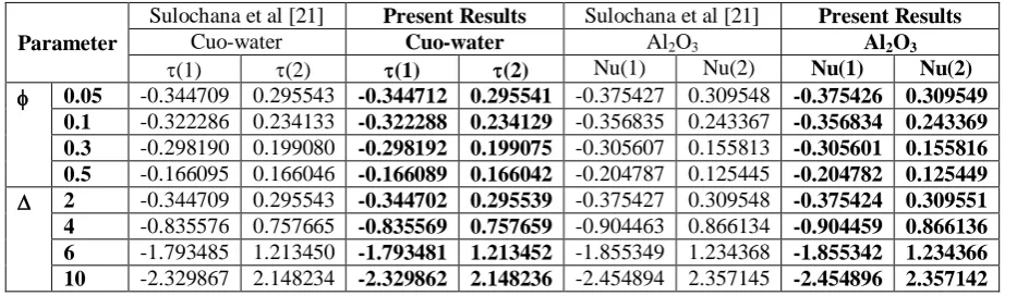
Comparison: In the absence of magnetic field (M=0), Thermal radiation (Rd=0) the results are in good agreement with

Sulochana et al. [21].

Parameter

Sulochana et al [21] Present Results Sulochana et al [21] Present Results

Cuo-water Cuo-water Al2O3 Al2O3

τ(1) τ(2) τ(1) τ(2) Nu(1) Nu(2) Nu(1) Nu(2)

φ 0.05 -0.344709 0.295543 -0.344712 0.295541 -0.375427 0.309548 -0.375426 0.309549

0.1 -0.322286 0.234133 -0.322288 0.234129 -0.356835 0.243367 -0.356834 0.243369 0.3 -0.298190 0.199080 -0.298192 0.199075 -0.305607 0.155813 -0.305601 0.155816 0.5 -0.166095 0.166046 -0.166089 0.166042 -0.204787 0.125445 -0.204782 0.125449 ∆ 2 -0.344709 0.295543 -0.344702 0.295539 -0.375427 0.309548 -0.375424 0.309551 4 -0.835576 0.757665 -0.835569 0.757659 -0.904463 0.866134 -0.904459 0.866136 6 -1.793485 1.213450 -1.793481 1.213452 -1.855349 1.234368 -1.855342 1.234366 10 -2.329867 2.148234 -2.329862 2.148236 -2.454894 2.357145 -2.454896 2.357142

6. RESULTS AND DISCUSSION

The equations governing the flow, heat and mass transfer have been solved by employing Galerkine finite element analysis with quadratic approximation polynomials. We have chosen here ∆=6.2 while M, D-1, α, Rd, φ,∆, are varied over a range, which are listed in the Figure legends.

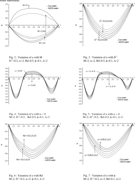
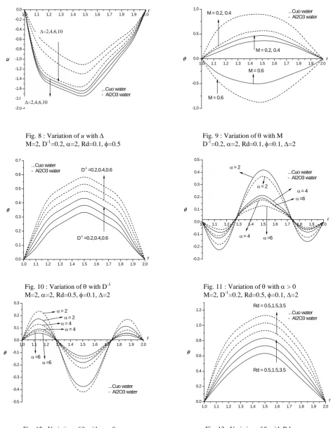
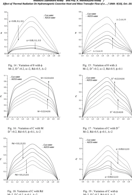
Fig.2 represents the effect of magnetic parameter M on the nanofluid velocity profile. It is observed from the figure that the velocity distribution increases with increasing magnetic parameter M≤4 and for higher M≥6, we notice a reduction in the velocity. This enhancement can be attributed to the fact that the magnetic field provides a resistive type of force known as the Lorentz force. This force tends to lessen the motion of the fluid for higher values of M≥ 6 as a consequence the velocity reduces. We also find that the nano-fluid velocity in the case of CuO – water nanofluid is relatively lesser than that of Al2O3-water nanofluid. This phenomenon has good agreement with the physical realities. Fig.9 represents the effect of magnetic parameter M on the nanofluid temperature profile. It is observed from the figure that the temperature distribution increases with increasing values of M≤4 and it ex h ibits a d ecreasing tend ency for higher M≥6,as a result of increase in the thickness of the thermal boundary layer owing to the Lorentz force developed by the magnetic field. We also find that the nano-fluid temperature in the case of CuO – water nanofluid is relatively greater than that of Al2O3-water nanofluid. This phenomenon has good agreement with the physical realities Fig.16 represents the effect of M on the nanofluid concentration profile. It is observed from the figure that the concentration distribution increases with increasing values of Mas a result of enhancement of the thickness of the solutal boundary layer. We also find that the nanofluid concentration in the case of CuO-water nanofluid is relatively lesser than that of Al2O3-water nanofluid. This phenomenon has good agreement with the physical realities.

Fig.3 represents the effect of inverse Darcy parameter D-1 on the nanofluid velocity profile. It is observed from the figure that the velocity distribution decreases with increasing the inverse Darcy parameter D-1. This is due to the fact that increase in the obstruction of the fluid motion with increase in the inverse Darcy parameter. We also find that the nano-fluid velocity in the case of CuO – water nanofluid is relatively lesser than that of Al2O3-water nanofluid. This phenomenon has good agreement with the physical realities. Fig.10 represents the effect of inverse Darcy parameter D-1 on the nanofluid temperature profile. It is observed from the figure that the temperature distribution increases with increasing values of D-1 as a result of increase in the thickness of the thermal boundary layer owing to the Darcy drag developed by the porous medium.. We also find that the nano-fluid temperature in the case of CuO – water nanofluid is relatively greater than that of Al2O3-water nanofluid. This phenomenon has good agreement with the physical realities Fig.17 represents the effect of inverse Darcy parameter D-1 on the nanofluid concentration profile. It is observed from the figure that the concentration distribution increases with increasing values of D-1 as a result of increasing the thickness of the solutal boundary layer owing to the Darcy drag developed by the porous medium. We also find that the nano-fluid concentration in the case of CuO-water nanofluid is relatively smaller than that of Al2O3-water nanofluid. This phenomenon has good agreement with the physical realities.

The variation of velocity with Radiation parameter (Rd) is exhibited in Fig.6. It is found that velocity shows an enhancement with increasing the values of Rd in the flow region. This is due to the fact that the thickness of the boundary layer increases with values of Rd in both types of nanofluids. Fig.13 shows the variation of temperature with Rd. It is found that an increase in Rd enhances the temperature in the thermal boundary layer. Thus lesser the radiative heat flux larger the temperature in the flow region. We also note that the temperature in Al2O3-water nanofluid is relatively smaller than that of CuO-water nanofluid.

Fig.7 display the effect of nanoparticle volume fraction φ on the nanofluid velocity. It is found that as the nanoparticle volume fraction decreases the nanofluid velocity in both types of nanofluids. These figures illustrate this agreement with the physical behaviour. When the volume of the nanoparticle reduces the thermal conductivity and hence reduces the momentum boundary layer thickness. We also notice that the nanofluid velocity in the case of Al2O3 – water nanofluid is relatively greater than that of CuO-water nanofluid. Fig.14 shows that the variation of temperature with φ. It can be seen from the profiles that an increase in the nanoparticle volume fraction reduces the temperature in the boundary layer. This is due to the fact that the thickness of the thermal boundary layer decreases with increase in φ. Also we find that the temperature in Al203-water is relatively lesser than that of CuO-water fluid. Fig.19 shows the variation of concentration with nanoparticle volume fraction φ.We notice a reduction in the concentration with increasing φ. This may be attributed to the fact that an enhancement in φ results in decreasing the thickness of the solutal boundary layer. The concentration in CuO-water nanofluid is smaller than those values of C in Al203-water nanofluid.

The variation of velocity with ∆ is exhibited in Fig.8. It is found that velocity shows an enhancement with increasing the values of ∆in the flow region. This is due to the fact that the thickness of the boundary layer increases with values of ∆ in both types of nanofluids. Fig.17 shows the variation of temperature with ∆. It is found that an increase in ∆ enhances the temperature in the thermal boundary layer. Thus lesser the thermal diffusivity larger the temperature in the flow region.. We also note that the temperature in Al2O3-water nanofluid is relatively smaller than that of CuO-water nanofluid.

The table 3 displays the behaviour of local skin friction (τ) at the inner and outer cylinders r=1&2. The variation of τ with magnetic parameter M & D-1shows that higher the Lorentz force /Lesser the permeability of the porous medium larger the skin friction at r=1&2 in both types of nanofluids. The rate of heat transfer on r=1&2 with increase in the strength of the heat generating/absorbing source. The Sherwood number reduces on r=1 with increase in the strength of the heat generating/absorption source while a reversed effect is noticed on the r=2. The rate of heat transfer reduces on the inner cylinder and enhances on the outer cylinder with increase in α>0 and in the case of α<0, a reversed effect is noticed in the behaviour of Nu on the both the cylinders.

The variation of τ with radiation parameter Rd shows that higher the radiative heat flux smaller the magnitude of the skin friction on the both walls. With respect to ∆, we find that lesser the thermal diffusivity, smaller the skin friction at both the cylinders in both types of nanofluid. From the tabular values of the skin friction with different parametric variations we find that the magnitude of skin friction in CuO-water nanofluid is relatively lesser than those values in Al2O3-water nanofluid. Also the magnitude of the skin friction at the inner cylinder is relatively larger than those on the outer cylinder for all variations.

The local Nusselt number (Nu) at the inner and outer cylinders r=1&2 is shown in table 3 for different parametric variations. The rate of heat transfer in the CuO-water nanofluid is relatively lesser than those values in Al2O3-water nanofluid. With respect to variation of Nu with magnetic parameter M we find that higher the Lorentz force/lesser the permeability of the porous medium larger the rate of heat transfer at r=1&2 in both types of nanofluids. We observed that the Nusselt number in CuO-water nanofluid is relatively smaller than those values in Al2O3-water nanofluid. The rate of heat transfer with radiation parameter Rd shows that higher the radiative heat flux larger the Nusselt number at both the cylinders. An increase in the Nanoparticle volume fraction φ reduces Nu at r=1&2 in CuO-water and Al2O3 -water nanofluids. The rate of heat transfer in the CuO--water nanofluid is relatively lesser than those values in Al2O3 -water nanofluid. The variation of Nu with Prandtl number Pr shows that |Nu| increases with increase in Pr.and |Nu| in CuO-water nanofluid are lesser than those values in Al2O3-water nanofluid.

smaller than those values in Al2O3-water nanofluid. With reference to Rd we find that the rate of mass transfer reduces with increasing values of Rd on both the cylinders in both types of nanofluids. The variation of Sh with Nano particle volume fraction φ shows that the rate of mass transfer reduces at r=1&2 with increase in φ in CuO-water and Al2O3 -water nanofluids.

1.0 1.1 1.2 1.3 1.4 1.5 1.6 1.7 1.8 1.9 2.0

-1.5 -1.0 -0.5 0.0 0.5 1.0 1.5

M = 2,4,6

...Cuo water - Al2O3 water

M = 2,4 u

M = 6

r

Fig. 2 : Variation of u with M

D-1=0.2, α=2, Rd=0.5, φ=0.1, ∆=2

1.0 1.1 1.2 1.3 1.4 1.5 1.6 1.7 1.8 1.9 2.0

-1.0 -0.8 -0.6 -0.4 -0.2 0.0

...Cuo water - Al2O3 water D-1

=0.2,0.4,0.6

u

D-1

=0.2,0.4,0.6

r

Fig. 3 : Variation of u with D-1 M=2, α=2, Rd=0.5, φ=0.1, ∆=2

1.0 1.1 1.2 1.3 1.4 1.5 1.6 1.7 1.8 1.9 2.0

-1.8 -1.6 -1.4 -1.2 -1.0 -0.8 -0.6 -0.4 -0.2 0.0 0.2 0.4 0.6

α = 2,4,6

...Cuo water - Al2O3 water α = 2,4,6

u

r

Fig. 4 : Variation of u with α > 0

M=2, D-1=0.2, Rd=0.5, φ=0.1, ∆=2

1.0 1.1 1.2 1.3 1.4 1.5 1.6 1.7 1.8 1.9 2.0

-1.8 -1.6 -1.4 -1.2 -1.0 -0.8 -0.6 -0.4 -0.2 0.0 0.2 0.4 0.6

α = -2,-4,-6

...Cuo water - Al2O3 water α = -2,-4,-6

u

r

Fig. 5 : Variation of u with α < 0 M=2, D-1=0.2, Rd=0.5, φ=0.1, ∆=2

1.0 1.1 1.2 1.3 1.4 1.5 1.6 1.7 1.8 1.9 2.0

-1.0 -0.8 -0.6 -0.4 -0.2 0.0

...Cuo water - Al2O3 water Rd = 0.5,1.5,3.5

u

Rd = 0.5,1.5,3.5

r

Fig. 6 : Variation of u with Rd

M=2, D-1=0.2, α=2, φ=0.1, ∆=2

1.0 1.1 1.2 1.3 1.4 1.5 1.6 1.7 1.8 1.9 2.0

-1.0 -0.8 -0.6 -0.4 -0.2 0.0

φ = 0.05,0.1,0.3

φ = 0.05,0.1,0.3

...Cuo water - Al2O3 water

u

r

1.0 1.1 1.2 1.3 1.4 1.5 1.6 1.7 1.8 1.9 2.0

-2.0 -1.8 -1.6 -1.4 -1.2 -1.0 -0.8 -0.6 -0.4 -0.2 0.0

Pr = 0.71,3.71,6.2

u

Pr = 0.71,3.71,6.2

r

...Cuo water - Al2O3 water

Fig. 8 : Variation of u with ∆ M=2, D-1=0.2, α=2, Rd=0.1, φ=0.5

∆=2,4,6,10

∆=2,4,6,10

1.0 1.1 1.2 1.3 1.4 1.5 1.6 1.7 1.8 1.9 2.0

-1.0 -0.5 0.0 0.5 1.0

M = 0.6 M = 0.2, 0.4

M = 0.6

M = 0.2, 0.4 ...Cuo water

- Al2O3 water

θ r

Fig. 9 : Variation of θ with M D-1=0.2, α=2, Rd=0.1, φ=0.1, ∆=2

1.0 1.1 1.2 1.3 1.4 1.5 1.6 1.7 1.8 1.9 2.0

0.0 0.1 0.2 0.3 0.4 0.5 0.6 0.7

...Cuo water

- Al2O3 water D-1

=0.2,0.4,0.6

θ

D-1 =0.2,0.4,0.6

r

Fig. 10 : Variation of θ with D-1

M=2, α=2, Rd=0.5, φ=0.1, ∆=2

1.0 1.1 1.2 1.3 1.4 1.5 1.6 1.7 1.8 1.9 2.0

-0.3 -0.2 -0.1 0.0 0.1 0.2 0.3 0.4 0.5

α = 4

α =6

α = 2

α = 2

...Cuo water - Al2O3 water

θ

r

α =6

α = 4

Fig. 11 : Variation of θ with α > 0 M=2, D-1=0.2, Rd=0.5, φ=0.1, ∆=2

1.0 1.1 1.2 1.3 1.4 1.5 1.6 1.7 1.8 1.9 2.0

-0.5 -0.4 -0.3 -0.2 -0.1 0.0 0.1 0.2 0.3

...Cuo water - Al2O3 water

θ

r

α = 2

α = 2

α = 4

α =6

α =6

α = 4

Fig. 12 : Variation of θ with α < 0

M=2, D-1=0.2, Rd=0.5, φ=0.1, ∆=2

1.0 1.1 1.2 1.3 1.4 1.5 1.6 1.7 1.8 1.9 2.0

0.0 0.2 0.4 0.6 0.8 1.0 1.2

...Cuo water - Al2O3 water

Rd = 0.5,1.5,3.5

θ

Rd = 0.5,1.5,3.5

r

1.0 1.1 1.2 1.3 1.4 1.5 1.6 1.7 1.8 1.9 2.0 0.0

0.1 0.2 0.3 0.4 0.5 0.6

φ = 0.05, 0.1, 0.3

φ = 0.05, 0.1, 0.3

...Cuo water - Al2O3 water

θ

r

Fig. 14 : Variation of θ with φ

M=2, D-1=0.2, α=2, Rd=0.5, ∆=2

1.0 1.1 1.2 1.3 1.4 1.5 1.6 1.7 1.8 1.9 2.0

0.0 0.1 0.2 0.3 0.4 0.5 0.6

...Cuo water - Al2O3 water

Pr = 0.71,3.71,6.2

θ

Pr = 0.71,3.71,6.2

r

Fig. 15 : Variation of θ with ∆ M=2, D-1=0.2, α=2, Rd=0.5, φ=0.1

∆=2,4,6,10

∆=2,4,6,10

1.0 1.1 1.2 1.3 1.4 1.5 1.6 1.7 1.8 1.9 2.0

0.0 0.1 0.2 0.3 0.4 0.5 0.6 0.7

M = 0.2,0.4,0.6 ...Cuo water

- Al2O3 water

C

M = 0.2,0.4,0.6

r

Fig. 16 : Variation of C with M

D-1=0.2, Rd=0.5, φ=0.1, ∆=2

1.0 1.1 1.2 1.3 1.4 1.5 1.6 1.7 1.8 1.9 2.0

0.0 0.1 0.2 0.3 0.4 0.5

D-1

=0.2,0.4,0.6 ...Cuo water

- Al2O3 water

D-1

=0.2,0.4,0.6

C

r

Fig. 17 : Variation of C with D-1 M=2, Rd=0.5, φ=0.1, ∆=2

1.0 1.1 1.2 1.3 1.4 1.5 1.6 1.7 1.8 1.9 2.0

0.0 0.1 0.2 0.3 0.4 0.5

...Cuo water - Al2O3 water

Rd = 0.5,1.5,3.5

C

Rd = 0.5,1.5,3.5

r

Fig. 18: Variation of C with Rd

M=2, D-1=0.2, φ=0.1, ∆=2

1.0 1.1 1.2 1.3 1.4 1.5 1.6 1.7 1.8 1.9 2.0

0.0 0.1 0.2 0.3 0.4

φ = 0.05,0.1,0.3 ...Cuo water

- Al2O3 water

φ = 0.05,0.1,0.3

C

r

Table--2: Skin Friction (τ) at the boundaries r = 1 and 2.

Parameter _τ(1) Cuo-water _{τ(2) τ(1)} Al2O3-water _τ(2)

M 0.5

1.5 3.0 -0.346 -0.397 -0.413 0.271 0.299 0.368 -0.347827 -0.399628 -0.530861 0.272488 0.300678 0.370653

D-1 0.2

0.4 0.6 -0.34 -0.376 -0.413 0.271 0.293 0.319 0.34827 -0.378611 -0.416042 0.272481 0.294481 0.321161 α 2 4 -2 -4 -0.23717 -0.23577 -0.23166 -0.23301 0.16968 0.16861 0,16547 0.16651 -0.238486 -0.236415 -0.230429 -0.232387 0.170687 0.169107 0.164534 0.166031

Rd 0.5

2.5 3.5 5.0 -0.346 -0.344 -0.343 -0.342 0.271 0.270 0.269 0.267 -0.34827 -0.34679 -0.347529 -0.347475 0.272484 0.272378 0.27227 0.272232

φ 0.05 0.1 0.3 0.5 -0.346 -0.268 -0.101 -0.058 0.271 0.133 0.080 0.046 -0.347828 -0.168935 -0.0731107 -0.0558487 0.272484 0.133677 0.058131 0.044451

∆ 2

4 6 10 -0.346 -0.835 -1.796 -3.329 0.271 0.655 1.410 2.618 -0.347824 -0.844163 -1.83489 -3.46394 0.272484 0.661346 1.43768 2.71458

Table – 3: Nusselt Number (Nu) at the boundaries r = 1 and 2.

Parameter Cuo-water Al2O3 -water

Nu (1) Nu (2) Nu (1) Nu (2)

M 0.5

1.5 3.0 0.21577 0.24774 0.32856 -0.1690 -0.1864 -0.2295 0.21665 0.248915 0.330656 -0.169721 -0.187283 -0.230868

D-1 0.2 0.4 0.6 0.2157 0.23476 0.25784 -0.1690 -0.1826 -0.1991 0.21665 0.235825 0.259139 -0.169721 -0.183425 -0.200041 α 2 4 -2 -4 -0.4166 -0.2066 0.4042 0.2036 0.2977 0.1477 -0.2885 -0.1454 -0.418512 -0.207154 0.402134 0.203057 0.299534 0.148175 -0.287137 -0.145076

Rd 0.5

1.5 3.5 5.0 0.21577 0.41708 0.56867 0.61932 -0.1690 -0.3269 -0.4459 -0.4856 0.21665 0.420377 0.626608 0.700219 -0.169721 -0.329331 -0.490914 -0.548591

φ 0.05 0.1 0.3 0.5 0.21577 0.10506 0.06348 0.03618 -0.1690 -0.0831 -0.0503 -0.0287 0.21665 0.105224 0.045538 0.034786 -0.169721 -0.832153 -0.362082 -0.276868

∆ 2

Table – 4: Sherwood Number (Sh) at the boundaries r = 1 and 2.

Parameter Cuo-water Al2O3-water

Sh (1) Sh (2) Sh (1) Sh (2)

M 0.5

1.5 3.0

0.219086 0.250915 0.330908

-0.158652 -0.179936 -0.233166

0.220067 0.252234 0.333139

0.15935 0.180842 0.234712

D-1 0.2 0.4 0.6

0.219086 0.240309 0.266106

-0.158652 -0.173749 -0.192088

0.220067 0.241491 0.267558

-0.15935 -0.174589 -0.193119

α 2

4 -2 -4

0.747845 0.760395 -0.787312 -0.785074

0.748776 0.758563 0.787312 0.777829

-0.736189 -0.754633 -0.808339 -0.790703

0.739688 0.754069 0.796016 0.782227

Rd 0.5

1.5 3.5 5.0

0.219086 0.218977 0.217305 0.217045

-0.158652 -0.157928 -0.157384 -0.157202

0.220067 0.219964 0.219863 0.219823

-0.15935 -0.15927 -0.159202 -0.159176

Sc 0.24 0.66 1.3

0.040446 0.111228 0.219086

-0.0292895 -0.0805462 -0.158652

0.0406278 0.112133 0.220067

-0.0294195 -0.0811948 -0.15935

γ 0.5

1.5 -0.5 -1.5

0.219086 0.0415453 0.0334789 0.0305212

-0.158652 -0.0300361 -0.0242815 -0.0221693

0.220067 0.246593 0.198714 0.181158

-0.15935 -0.178267 -0.144114 -0.131572

φ 0.05 0.1 0.3 0.5

0.219086 0.106332 0.0641656 0.0365028

-0.158652 -0.077171 -0.0466089 -0.0265309

0.220067 0.106509 0.045996 0.0351252

-0.15935 -0.0772964 -0.0334261 -0.0255302

∆ 2

4 6 10

0.219086 0.528328 1.13396 2.09737

-0.158652 -0.382636 -0.821456 -1.519998

0.220067 0.534066 1.16069 2.19075

-0.15935 -0.386715 -0.840484 -1.586456

7. CONCLUSIONS

The coupled equations governing the flow, heat and mass transfer have been solved by using Galerkin finite method with quadratic approximation functions. The velocity, temperature and concentration have been analysed for different parametric variations. The important conclusions of the analysis are

 Higher the Lorentz force smaller the velocity and temperature, larger the concentration. The skin friction, the rate of heat and mass transfer reduces on the cylinders with increase in M.

 The velocity, temperature enhances while the concentration reduces with increase in the strength of the heat generating source and in the case of heat absorption source, the velocity reduces, the temperature and concentration enhances in the flow region. The skin friction enhances with increase in α>0 and reduces with α<0 on both the cylinders. The rate of heat transfer on r=1&2 with increase in the strength of the heat generating/absorbing source. The Sherwood number reduces on r=1 with increase in the strength of the heat generating/absorption source while a reversed effect is noticed on the r=2. The rate of heat transfer reduces on the inner cylinder and enhances on the outer cylinder with increase in α>0 and in the case of α<0, a reversed effect is noticed in the behaviour of Nu on the both the cylinders.

 An increasing Rd increases velocity and temperature.

 An increase in nano particle concentration reduces a velocity, temperature and concentration.

8. REFERENCES

1. Abu-Nada, E., Masoud, Z., Hijazi, A: Natural convection heat transfer enhancement in horizontal concentric annuli using nanofluids, Int Commun Heat Mass Transf, V.35, 657-665(2008),

2. Abu-Nada, E: Effect of variable viscosity and thermal conductivity of Al2O3-water nanofluid on heat transfer enhancement in natural convection, Int J heat Fluid Flow, V.30, 679-690(2009).

3. Behzadmehr, A., Saffar-Avval, M., Galanis, N: Prediction of turbulent forced convection of a nanofluid in a tube with uniform heat flux using a two phase approach, Int J Heat Fluid Flow, V.28, 211-219(2007).

4. Bianco V., Chiacchio. F., Manca, O., Nardini, S: Numerical investigation of nanofluids forced convection in circular tubes, J. Appl Therm Eng, V.29, 3632-3642(2009).

5. Choi, S.U.S: Enhancing thermal conductivity of fluid with nanoparticles, developments and applications of non-Newtonian flow, ASME FED 231, 99-105(1995).

6. Das, S., Jana, R.N., and Makinde, O.D : Mixed convective magneto hydrodynamic flow in a vertical channel filled with nanofluids, Engineering science and technology an International Journal, V.18, 244-255(2015). 7. Jou, R.Y., Tzeng, S. C: Numerical research of nature convective heat transfer enhancement filled with

nanofluids in rectangular enclosures, Int Commun Heat Mass Transf, V.33, 727-736(2006).

8. Kuhen TH, Goldstein RJ: An experimental and theoretical study of natural convection in the annulus between horizontal concentric cylinders, J. Fluid Mech, 74, 695-719 (1976).

9. Kuhen TH, Goldstein RJ: An experimental study of natural convection heat transfer in concentric and eccentric horizontal cylindrical annuli, ASME J Heat Transfer, V.100, 635-640 (1978).

10. Madhusudhana Reddy, Y., Rama Krishna, G.N. and Prasada Rao, D.R.V: Numerical study of Convective Flow of CuO-water and Al2O3-water nanofluids in cylindrical annulus, Int. Journal of Research & Development in Tech., Vol. 7, Issue 3, 142-148 (2017).

11. Maxwell J.C: Electricity and magnetism, Clarendon Press, Oxford, UK (1873).

12. Mokhtari Moghari, R., Akbarinia, A., Shariat, M., Talebi, F., Laur, R: Two phase mixed convection Al2O3 -water nanofluid flow in an annulus, Int J Multiph Flow, V. 37(6), 585-595(2011).

13. Nagasasikala, M and Phrabhakar Rao G: Heat and mass transfer of a MHD flow of a nanofluid through a porous medium in an annular, circular region with outer cylinder maintained at constant heat flux, Presented in NCIT Conference, SSBN Degree College, Ananatapuramu (2016).

14. Parvin, S., Nasrin, R., Alim, M.A., Hossain, N.F., Chamka, A. J: Thermal conductivity variation on natural convection flow of water-alumina nanofluid in an annulus, Int J Heat Mass Transf, V.55 (19-20), 5268-5274(2012).

15. Putra, N., Roetzel W, Das, S.K: Natural convection of nanofluids, Heat and Mass Transfer, V.39 (8-9), 775-784(2003).

16. Santra, A.K., Sen, S., Chakraborty., N: Study of heat transfer due to laminar flow of copper-water nanofluid through two iso-thermally heated parallel plates, Int J Therm Sci., V.48, 391-400(2009).

17. Soleimani, S.I., Sheikholeslami, M., Ganji, D.D., Gorji-Bandpay, M: Natural convection heat transfer in a nanofluid filled semi annulus enclosure, Int Commun Heat Mass Transf, V.39 (4), 565-574(2012).

18. Sree Devi, G., Raghavendra Rao, R., Chamka, A.J and Prasada Rao, D.R.V: Mixed convective heat and mass transfer flow of nanofluids in concentric annulus with constant heat flux, Procedia Engineering, 127, 1048-1055(2015).

19. Srinivas, G., Srikanth Gorti, V.P.N., Suresh Babu, B and Sreenatha Reddy, S: Particle spacing and chemical reaction effects on convective heat transfer through a nanofluid in cylindrical annulus, Procedia Engineering, 127, 263-270 (2015).

20. Sudarsana Reddy, P., Chamka, A.J: Soret and Dufour effects on MHD convective flow of Al2O3-water and TiO2- water nanofluids past a stretching sheet in porous media with heat generation/absorption, J. Advanced Powder Technology, V. 27, 1207-1218(2016).

21. Suochana G and Ramakrishna G N : Effect of Heat Sources on Non-Darcy Convective Heat and Mass Transfer Flow of Nanofluids in Cylindrical Annulus, International Journal of Mathematical Archive (IJMA), Issue 6, Vol. 8, pp. 53-62 (2017), ISSN 2229-5046.

22. Wen, D and Ding, Y: Formulation of nanofluids for natural convective heat transfer applications, Int J Heat Fluid Flow, V. 26(6), 855-864(2005).

Source of support: Nil, Conflict of interest: None Declared.