Applying inventory classification to a large inventory management system

(1)

ISSN: 1984-3046 © JOSCM | São Paulo | V. 10 | n. 1 | Jan-June 2017 |68-86

ARTICLES

Submitted 29.10.2016. Approved 07.03.2017.

Evaluated by double blind review process. Scientific Editor: Nelson Kuwahara

DOI: http:///dx.doi/10.12660/joscmv10n1p68-86

APPLYING INVENTORY CLASSIFICATION TO A

LARGE INVENTORY MANAGEMENT SYSTEM

AbSTRACT

Inventory classification aims to ensure that business-driving inventory items are ef-ficiently managed in spite of constrained resources. There are numerous single- and multiple-criteria approaches to it. Our objective is to improve resource allocation to focus on items that can lead to high equipment availability. This concern is typical of many service industries such as military logistics, airlines, amusement parks and public works. Our study tests several inventory prioritization techniques and finds that a modified multi-criterion weighted non-linear optimization (WNO) technique is a powerful approach for classifying inventory, outperforming traditional tech-niques of inventory prioritization such as ABC analysis in a variety of performance objectives.

KEYWORDS | Multi-criteria inventory classification, priority schemes, ABC analysis, nonlinear programming, spare parts management.

benjamin Isaac May [email protected]

Supply Analyst at US Navy, Weapon Systems Support – Philadelphia, PA, USA

Michael P. Atkinson [email protected]

Professor at Naval Postgraduate School, Department of Operations Research – Monterey – CA, USA

Geraldo Ferrer [email protected]

(2)

ISSN: 1984-3046 © joScm | São Paulo | V. 10 | n. 1 | jan-june 2017 | 68-86

INTRODUCTION

The logistics unit of a large navy is denominated WSS (weapons system support). It is responsible for spare parts support for all maritime and aviation assets in this military force. This support includes procure-ment, production, repair, and transportation. The unit’s responsibility is uniquely complex relative to other military or civilian organizations due to the size of its inventory (400,000+ unique parts) and its multi-item, multi-indenture, multi-echelon inventory system. The WSS planners individually analyze and plan (both long-term and short-term) the supply for each spare part. Once the support plan is determined, contracting specialists place that stock-keeping unit (SKU) on production or repair contracts, a decision based on vendor, budget, and other variables for each item. Planners and contracting specialists cur-rently respond to each part requirement, primarily, on a first-come-first-serve basis. The current system does not allocate limited resources, time and budget, to the items most important to operations. If there are immediate operational needs, supply officers con-tact WSS to request prioritization of certain items, re-gardless of their attributes. The suboptimal resource allocation leads to less-than-ideal performance on key metrics, such as fill rate (fraction of initial orders fulfilled from stock), delay (time to release material for shipment), backorders (unfilled orders awaiting fulfillment), and response time (time between req-uisition and delivery). This multi-criterion decision making process impacts equipment availability, the primary goal of the enterprise.

To increase fill rate of its maritime inventory, WSS is implementing a four-category inventory classification system called WSS4. The goal of this system is to fo-cus WSS resources on items in the highest category to minimize the unfilled orders on those items. The system considers demand and two other factors to classify items: casualty reports (CASREP) and platform readiness drivers.CASREP are emergency requisitions for parts required to fix a system that is critical to a mission. Platform readiness drivers areitems that were identified as problematic, either because of their im-pact on equipment availability or because their sup-ply chain is unreliable. The system considers only demand, casualty reports, and platform readiness drivers to group items into the four categories, but the thresholds used to define the boundaries of these categories are set by inventory managers, based on what they deem a manageable workload within each group.

Although the WSS4 method adopts some prioritiza-tion, there are other factors that influence equipment availability. A model that considers only requisitions and CASREP may not be the best technique for im-proving resource allocation.

This study evaluates existing inventory prioritization methods and compares them against WSS4, the meth-od currently in use. Before we present other methmeth-ods, we briefly introduce ABC Analysis, the seminal inven-tory categorization technique.

Research objective

The purpose of this study is to determine an effective classification approach for a large spare parts inven-tory management system by comparing some of the classification methods in the literature. We use input from inventory planners to identify the factors that have most significant impact on WSS’s primary goal, equipment availability. Based on those factors, an ABC-like model is tailored for WSS inventory man-agement needs. Once the model is built, we test it with inventory data collected by the ERP system. The model is contrasted with alternative prioritization schemes, including the WSS4 method being imple-mented by WSS. Raw spare parts demand data for this study was provided by WSS.

The remainder of this paper is organized as follows: Section presents the literature of inventory pri-oritization with focus on the approaches used in our analysis. Section 3 overviews the data selected for testing our prioritization model. Section 4 presents a subset of the many variables available for each trans-action in the ERP. The section culminates in subsec-tion 4.6 where we present the final variable selecsubsec-tion, supported by the expert judgement of WSS inventory planners. Section 5 explains the methodology behind the WNO approach to inventory prioritization, fol-lowed by the WNO model analysis in Section 6. Sub-section 6.2 compares the WNO model with other in-ventory prioritization approaches. It shows that the WNO model outperforms all other multi-criterion ap-proaches in a variety of performance metrics. Section 7 discusses the analysis.

LITERATURE REVIEW

(3)

stock items into different levels of management at-tention. It is based on Pareto’s law, which states that the significant items in a group usually constitute only a small fraction of the total number of items in that group (Zimmerman 1975). Pareto’s law can be applied to many fields of study, and is particularly ap-plicable to inventory management. ABC uses a single dimension, demand value, the product of demand rate and unit price, as its primary metric (Silver et al. 1998). The reasoning is that there are a finite number of dollars available for inventory management, and those dollars must be used wisely.

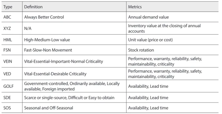
Spare parts inventories can be extremely difficult to manage. The ABC analysis is the first of many clas-sification schemes used by inventory managers. By focusing on the business drivers, the ABC classifica-tion method allows businesses to significantly reduce inventory costs while minimizing stock-out rates. Other methods may focus on different metrics, and their applicability varies, as shown in Table 1 (Go-palakrishnan 2004). With business models varying across industries, these methods are often tailored to fit specific needs.

Table 1. AbC-derived classification techniques (Gopalakrishnan 2004)

Type Definition Metrics

ABC Always Better Control Annual demand value

XYZ N/A Inventory value at the closing of annual _accounts

HML High-Medium-Low value Unit value (price or cost)

FSN Fast-Slow-Non Movement Stock rotation

VEIN Vital-Essential-Important-Normal Criticality Performance, warranty, reliability, safety, _{maintainability, criticality}

VED Vital-Essential-Desirable Criticality Performance, warranty, reliability, safety, _{maintainability, criticality}

GOLF Government-controlled, Ordinarily available, Locally _{available, Foreign imported} Availability, Lead time

SDE Scarce or single-source, Difficult or Easy to obtain Availability, Lead time

SOS Seasonal and Off-Seasonal Availability, Lead time

As business models evolved and computing power increased, complex multi-criteria inventory models were developed. Regardless of the model most appli-cable to a particular business, Pareto’s law remains the underlying principle behind most inventory classifica-tion techniques in use today. This paper explores al-ternative factors that may provide more value to man-aging spare parts than just targeting fill rates.

Pareto’s law is the original theory behind the ABC inventory management technique. Some advanced multi-criteria inventory classification (MCIC) varia-tions have been developed using the Pareto principle. They aim to achieve the same goal of prioritizing items either on a categorical or individual basis. We explore eight specific multi-dimensional models in detail re-garding their applicability to WSS business require-ments. These variants include joint-criteria matrix,

MUSIC-3D, operations-related groups, analytic hier-archy process, genetic algorithm for multi-criteria in-ventory classification, weighted linear optimization, simple classifiers for multiple-criteria ABC analysis, and weighted non-linear optimization models.

(4)

critical-ISSN: 1984-3046 © JOSCM | São Paulo | V. 10 | n. 1 | Jan-June 2017 | 68-86

ity). Items not directly falling on one of the diagonal categories (“AA”, “BB”, or “CC”) are subjectively moved to the diagonal category best representing their pri-ority (Flores and Whybark 1987). Th is approach is reasonable with two factors (demand value and criti-cality), but it becomes more unwieldy with more fac-tors. Our multi-factor analysis overcomes these limi-tations.

Gopalakrishnan introduced the MUSIC-3D model as a 3-D matrix focusing on fi nance, operations, and criticality. Each of the three dimensions is split in two levels: “High/Low consumption value (HCV/LCV)”, “Long/Short Lead Time (LLT/SLT)” and “Critical/ Non-critical (C/NC)”. Each item in inventory is clas-sifi ed and located in one of the eight 3D cells such as LCV-NC-LLT. Th e cells are ranked one dimension at a time, such that all HCV items are ranked higher than LCV items. Among HCV (or LCV) items, all Criti-cal items are ranked higher than Non-critiCriti-cal items. Finally, among Critical (or Non-Critical) items, all LLT items are ranked higher than SLT items. Conse-quently, the cells are ranked following the sequence: HCV-C-LLT, HCV-C-SLT, HCV-NC-LLT, …, and LCV-NC-SLT. Th is classifi cation is quite subjective, but it is easy to implement (Gopalakrishnan 2004). As with the joint-criteria model, this approach does not scale well with additional factors and requires a certain amount of subjective ranking by the decision maker.

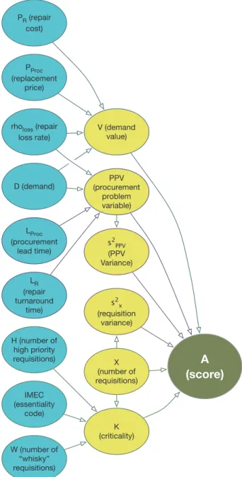
Cohen and Ernst introduced Operations-Related Groups as another MCIC method. Inventory items are clustered based on statistical procedures using operational constraints such as market attributes, production- and distribution-related parameters, and fi nancial data to minimize the impact resulting from the shortage of a few items (Cohen and Ernst 1988). Flores, Olson and Dorai applied Saaty’s Analytic Hier-archy Process (AHP) as yet another MCIC method. Th e AHP arranges complex and unstructured data into a hierarchy of nodes with branches, and assigns relative weights to specifi ed item criteria, which are then used to create and assign scores to inventory items (Saaty 1977, Flores et al. 1992). Items are ranked based on their scores. Figure 1 shows the initial structure of AHP applied to inventory categorization. Th ree crite-ria make up “criticality,” while four critecrite-ria, including “criticality,” make up “utility.” A “relative importance” scale could be used to assign values to the criteria. Scores for each item would then be calculated, and the items’ score would be used to prioritize them. Our primary approach has similarities to AHP in that we score each item based on a weighted sum of criteria.

We determine the weights using a diff erent method that does not require the pairwise comparisons in AHP.

Figure 1. AHP Structure (Flores et al. 1992).

Artifi cial Neural Networks (ANN) and Genetic Al-gorithm for Multi-criteria Inventory Classifi cation (GAMIC) use genetic algorithms to build upon the AHP method. Th ey have been used to alleviate a few of the assumptions and restrictions of AHP, such as measurement of units of criteria and subjective scale assignments, creating consistency between com-parisons (Guvenir and Erel 1998). It is able to detect and extract nonlinear relationships and interactions among predictor variables (Partovi and Murugan 2002). GAMIC relaxes these assumptions by using a sample of classifi ed items to assign criteria weights.

Ramanathan introduced Weighted Linear Optimi-zation (WLO), a weighted additive function used to aggregate the performance of an inventory item, in terms of diff erent criteria, to a single optimal in-ventory score (Ramanathan 2006). To eliminate the requirement for optimization software while also providing comparable results, a Simple Classifi er for Multiple-Criteria (SCMC) analysis was created (Ng 2007). Th is model also converts all criteria measures into a scalar score, but it diff ers from WLO by trans-forming the criteria to a comparable base.

(5)

the model is simple enough to run without advanced software, it has the flexibility to add and change con-straints and factors as needed. Similar attempts to multi-criteria inventory classification (MCIC) include (Bacchetti et al. 2013, Hatefi et al. 2014, Lolli et al. 2014, Millstein et al. 2014, Park et al. 2014, Roda et al. 2014, Soylu and Akyol 2014, Babai et al. 2015).

DATA OVERVIEW

In this large organization, WSS is responsible for pro-viding wholesale- and retail-level support for both maritime and aviation platforms. The introduction of a new enterprise resource planning (ERP) system provided the organization with a single interface to manage its entire inventory, with the ability to track all aspects of parts flow through the organization’s multi-indenture, multi-echelon inventory distribu-tion structure. We filtered the data to include just the spare parts for maritime operations with demand over the three-year period from April 2011 through March 2014. Items that did not receive any order dur-ing that period were excluded from the analysis. We also used the item’s maturity as filter. Maritime items experience five life-cycle phases: initial operational ca-pability, pre-material support date, demand develop-ment interval, maturity, and sunset. Most items are in the mature life-cycle phase, and we only included these in our analysis.

In summary, of the 272,000 WSS-managed maritime items, 131,000 items are in the mature phase of their life cycles. By restricting to a demand history of at least one unit in the specified three-year time frame, only 17,587 items remained in our sample.

Relevant attributes

The reports provided by the ERP include more than 70 different attributes for each item in the system. These attributes are organized in five data categories: demand, lead times, repair capability, price, and clas-sifications. As expected, demand has a significant in-fluence on equipment availability. The primary vari-ables associated with demand are demand forecast, demand deviation (forecast error), requisition fre-quency, requisition size, regeneration demand, and attrition demand. Demand forecast is the expected demand of an item, obtained by analyzing its time-se-ries. Demand deviation is a measure of forecast error.

Requisition size and requisition frequency represent the average number of units per order and the number of orders per quarter, respectively. Regeneration demand

is the fraction of demand fulfilled with the repair of recycled items, while attrition demand is the fraction of demand fulfilled with the purchase of new items.

The next category, lead time, includes the average time and its sigma (deviation) for procurement, produc-tion, procurement administrative, repair, and repair administrative. These times represent the expected delays associated with particular portions of the sup-ply chain. These parameters are used for setting in-ventory safety levels and demand forecasts.

The repair capability category includes forecasts for item survival, carcass (i.e., an item requiring repair) return, and pipeline loss. Survival rate represents the probability that a carcass is repaired successfully by the repair facility. Carcass return rate represents the probability that inoperable items are returned to the repair facility. Pipeline loss rate represents the fraction of carcasses that is lost due to repair and non-repair reasons.

Numerous prices are associated with each item, in-cluding standard, net, replacement, and repair. They measure a part’s reparability, the cost to repair it, and the cost to replace it. Standard and net prices repre-sent incoming revenue for WSS from internal trans-actions. Replacement and repair prices represent costs due to external transactions. The standard price of an item is charged to the customer’s budget in the fleet for either a consumable part or a repairable part with no carcass turn-in. Net price is the rebate price charged to the customer when a carcass turn-in is provided as part of the transaction. Replacement and repair prices

are those paid by WSS to replace and repair the inven-tory items, respectively.

The classification category is the largest portion of ERP’s metadata. Classes, indicators, codes, identi-fiers, symbols, routers, and flags comprise approxi-mately half of the data fields.

VARIABLE SELECTION

In this section we determine which item attributes to include in our analysis to prioritize items for re-source allocation. We use a combination of regression analysis and subject matter expertise to determine the drivers of WSS’s primary goals, fill rate and equip-ment availability.

(6)

forests” approach (Breiman 2001, Benyami 2012), a machine learning method that combines the qualities of advanced cluster analysis with regression analysis to classify observations and prioritize factors. It gen-erates a multitude of decision trees from random data points in a large dataset, where each tree represents a predictive modeling approach to map an item’s quali-ties (predictor variables) to its dependent (response) variable.

For each tree in a random forest, a subset of random observations from a full observation set is chosen, and from these observations, random subsets of predictor variables are selected. An optimal bina-ry split is made on each branch using the variable that best impacts the specified objective function. This process is repeated multiple times, decreas-ing the mean squared residual error at each split. The final product represents one tree in the forest. Ultimately, the random selections of observations and predictor variables produce an ensemble of independently constructed trees. Once the forest is fully assembled, the node split values are aggre-gated and used to create classification criteria. The variables are ranked against each other based on how often and at what level they were chosen as the node’s best binary split variable. Because the objective of this analysis is to identify and verify the key variables driving fill rate, the relative rank-ing of variables is the primary goal of our random forest analysis.

The objective of random forest construction is to minimize the error in predicting the fill rate based on item parameters. We construct random forests of 1,000 trees for full observation of the 17,587 items in our sample. We use fill rate (drawn from compiled sales document data) as the response variable. We start by including all available variables (70+ fields) as predictors. We then proceed in an iterative manual process of removing variables and rebuilding trees to narrow our set of relevant variables. We use common sense, item manager advice, and WSS analyst recom-mendations to further refine our list of variables and confirm that the random forest suggestions are rea-sonable. This iterative process allowed us to remove variables with limited significance for this study and highlight the relative importance of the remaining variables. We finally converge on variables associated with price, criticality, and the mean and variance of demand and lead-time as the most important factors.

In the following subsections we describe the variables

of interest for the period 04/2011 to 03/2014 to de-termine their applicability and contribution to a pri-oritization model. Specific categories include fill rate, demand, lead time, criticality, and price. Each catego-ry includes several variables.

Fill rate

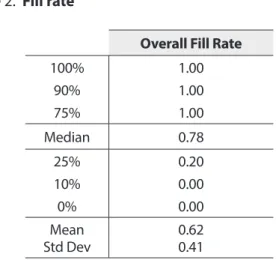
Fill rate (FR), the response variable, is the fraction of requisitions immediately filled with on-hand inven-tory. It is the primary performance measure for WSS because it relates to all other customer-oriented met-rics (such as average delay, backorders, and response time). The fill rate for an item is calculated by averag-ing the hit/miss binary values for each requisition. Ta-ble 2 displays the 36-month histogram for the 17,587 items in our analysis. It shows that the median fill rate was 78% and the mean was 62%, substantially lower than the 85% goal. All items in the upper quar-tile had a fill rate of 100%, but the lower quarquar-tile had a fill rate of 20% or less.

Table 2. Fill rate

Overall Fill Rate

100% 90% 75%

1.00 1.00 1.00

Median 0.78

25% 10% 0%

0.20 0.00 0.00 Mean

Std Dev 0.620.41

Demand

(7)

Table 3. Number of requisitions per item

Requisitions

100% 90% 75%

4871 27 10

Median 3

25% 10% 0%

1 1 1 Mean

Std Dev 13.672.6

A repair program refurbishes used assets to reis-sue them for future use. In most cases, expen-sive parts may be repaired at much lower cost than completely replacing them (Ferrer and Guide 2002). Survival rate and pipeline loss rate measure the reparability of a particular item. Repair surviv-al rate (ρR) is the fraction of assets that experience

a repair attempt and are successfully repaired. Table 4 shows a median repair survival rate of 90% and the mean is 67%. Repair pipeline loss rate (_ρ_LOSS) represents the fraction of assets in the re-pair pipeline that cannot be rere-paired. The pipeline loss rate table shows that the median ρLOSS is 13%,

meaning that more than half of the items in the dataset had less than 13% of the requisitions not repaired by the system.

Table 4. Repair survival rate and Pipeline loss rate

Repair survival rate Pipeline loss rate

100% 90% 75%

1.00 1.00 0.92

1.00 1.00 0.99

Median 0.90 0.13

25% 10% 0%

0.01 0.00 0.00

0.09 0.03 0.01 Mean

Std Dev 0.670.41 0.350.45

Demand (D) represents the annual demand for that item. The majority of the variables of interest relate to demand, not requisitions. Specific demand mea-sures include quantity demanded, demand deviation, regeneration demand, and attrition demand. Table 5 displays the relevant information. One item faced de-mand of 40,567, but the dede-mand for 90% of the items was lower than 39 in the 36-month period, and the median demand was 4.

Table 5. Demand, Demand deviation, Regeneration, and Attrition

Demand Demand deviation Regeneration demand Attrition demand

100% 90% 75%

40567 39 12

2167.77 2.85 1.14

1646.76 2.49 0.82

15423.00 2.63 0.48

Median 4 0.51 0.24 0.12

25% 10% 0%

2 1 0

0.22 0.00 0.00

0.00 0.00 0.00

0.03 0.00 0.00 Mean

Std Dev

38.41 486.11

3.51 37.23

1.46 15.56

8.78 165.86

The demand deviation(ε) is measured as a forecast er-ror. It indicates the difficulty in forecasting demand for low-demand items. Though coefficient of varia-tion (the ratio between the mean demand and its standard deviation) might be a better measure of rela-tive uncertainty, forecast error is tracked by the ERP and is easy to obtain, so it is the uncertainty metric used throughout this analysis. Regeneration demand (D_R) is the demand fulfilled through repair, while at-trition demand (D_ATT) is the demand fulfilled with new

purchases. These values play a large role in budget planning due to the high cost associated with pur-chasing new items. They reflect the importance of the repair pipeline.

Lead time

(8)

turn-ISSN: 1984-3046 © joScm | São Paulo | V. 10 | n. 1 | jan-june 2017 | 68-86

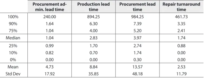
around lead times. Procurement administrative lead time (L_ADM) is the time it takes to award a procurement contract to a supplier. The clock starts when the con-tracting office receives a purchase request, and ends when the contract is awarded. Production lead time (L_PROD) is the time that it takes to manufacture and deliver a purchase order. Procurement lead time (L_PROC)

is the sum of the procurement administrative and production lead times. Repair turnaround time (L_R) is the time required to repair and deliver a repair order. Table 6 shows that the median lead times for each of the processes are relatively low, but their standard de-viations are high.

Table 6. Procurement administrative, Production, Procurement, and Repair time (days)

Procurement

ad-min. lead time Production lead time Procurement lead time Repair turnaround time

100% 90% 75%

240.00 1.64 1.04

894.25 6.30 4.00

984.25 7.39 5.20

461.73 3.35 2.41

Median 1.04 2.83 3.97 1.74

25% 10% 0%

0.99 0.82 0.00

1.70 0.70 0.00

2.74 1.74 0.30

0.88 0.00 0.00 Mean

Std Dev

4.73 17.92

8.84 35.85

13.57 48.18

2.53 11.79

Procurement problem variable (PPV) is a strong indica-tor of supply chain health for a particular item, and is defined in equation (1). It captures how much de-mand occurs while waiting for an ordered part (either

via replacement or repair). PPV identifies potential issues in the supply chain resulting from higher-than-forecasted demand and/or longer-than-expected lead times.

Table 6. Procurement administrative, Production, Procurement, and Repair time (days)

Procurement

admin. lead time Production lead time Procurement lead time turnaround time Repair

100% 240.00 894.25 984.25 461.73

90% 1.64 6.30 7.39 3.35

75% 1.04 4.00 5.20 2.41

Median 1.04 2.83 3.97 1.74

25% 0.99 1.70 2.74 0.88

10% 0.82 0.70 1.74 0.00

0% 0.00 0.00 0.30 0.00

Mean 4.73 8.84 13.57 2.53

Std Dev 17.92 35.85 48.18 11.79

Procurement problem variable (𝑃𝑃𝑃𝑃𝑃𝑃) is a strong indicator of supply chain health for a particular item, and is defined in equation (1). It captures how much demand occurs while waiting for an ordered part (either via replacement or repair). PPV identifies potential issues in the supply chain resulting from higher-than-forecasted demand and/or longer-than-expected lead times.

𝑃𝑃𝑃𝑃𝑃𝑃 = 𝐷𝐷 ∗ 𝐿𝐿𝑃𝑃𝑃𝑃𝑃𝑃𝐶𝐶∗ 𝜌𝜌𝐿𝐿𝑃𝑃𝐿𝐿𝐿𝐿+ 𝐷𝐷 ∗ 𝐿𝐿𝑃𝑃∗ (1 − 𝜌𝜌𝐿𝐿𝑃𝑃𝐿𝐿𝐿𝐿) (1) Table 7 provides the statistics for PPV and PPV variance (𝜎𝜎𝑃𝑃𝑃𝑃𝑃𝑃2 ). Once again, a small number of items is responsible for most cases of high PPV and high PPV variance values.Table 7 provides the statistics for PPV and PPV

vari-ance

Procurement

100% 240.00 894.25 984.25 461.73

90% 1.64 6.30 7.39 3.35

75% 1.04 4.00 5.20 2.41

Median 1.04 2.83 3.97 1.74

25% 0.99 1.70 2.74 0.88

10% 0.82 0.70 1.74 0.00

0% 0.00 0.00 0.30 0.00

Mean 4.73 8.84 13.57 2.53

Std Dev 17.92 35.85 48.18 11.79

𝑃𝑃𝑃𝑃𝑃𝑃 = 𝐷𝐷 ∗ 𝐿𝐿𝑃𝑃𝑃𝑃𝑃𝑃𝐶𝐶∗ 𝜌𝜌𝐿𝐿𝑃𝑃𝐿𝐿𝐿𝐿+ 𝐷𝐷 ∗ 𝐿𝐿𝑃𝑃∗ (1 − 𝜌𝜌𝐿𝐿𝑃𝑃𝐿𝐿𝐿𝐿) (1) Table 7 provides the statistics for PPV and PPV variance (𝜎𝜎𝑃𝑃𝑃𝑃𝑃𝑃2 ). Once again, a small number of items is responsible for most cases of high PPV and high PPV variance values.

. Once again, a small number of items is responsible for most cases of high PPV and high PPV variance values.

Table 7. PPV and PPV variance

Procurement

problem variable PPV variance

100% 90% 75%

15423.00 6.73 1.89

6.80E+07 31.39

4.46

Median 0.63 0.88

25% 10% 0%

0.21 0.02 0.00

0.21 0.00 0.00 Mean

Std Dev

10.24 166.69

8977.81 539085.25

Criticality

The notion of criticality plays a major role in repair parts management. Though a high level of demand

indicates that the item is frequently needed, its criti-cality could range from insignificant to vital. For in-stance, consider two types of light bulbs. The first has an annual demand of 50,000 units because it fits ev-ery reading light socket in a ship. Without the bulb, one needs another light source for reading. The sec-ond bulb has a demand of just 5 units per year, but it lights a control panel required for safe navigation. Without the second bulb, that panel is out of commis-sion. Though both types are important, the second bulb is critical to operational effectiveness and should be managed more carefully than first bulb.

Three types of criticality measures used for this analy-sis: “whisky” (w = 0 or 1) requisitions, requisition pri-orities (H = 0 or 1), and item management essentiality codes (IMEC = 0-5), as follow:

(9)

a ship from achieving its mission. Approximately 7% of all requisitions analyzed were classified as

w. The first column in Table 8 shows that, while one particular item suffered 548 whisky requisi-tions, more than half of the items had none. The last column shows that the urgency of the whisky process has an impact, but it is somewhat limited: the mean fill rate of whisky requisitions is just 75%, compared to the 62% overall fill rate shown in Table 2.

Table 8. Whisky requisitions, Whisky fraction, and Fill Rate

Whisky requisitions

Whisky requisition

fraction

Whisky fill rate

100% 90% 75%

548 4 1

1.00 0.67 0.29

1.00 1.00 1.00

Median 0 0.00 1.00

25% 10% 0%

0 0 0

0.00 0.00 0.00

0.50 0.00 0.00 Mean

Std Dev

1.82 7.06

0.18 0.30

0.75 0.39

2. Requisition priority: Requisitions contain a prior-ity code to identify the current operational status and its need for the part. It is derived as a com-bination of two variables – operational state and urgency – to indicate if the requisition is high pri-ority. Table 9 provides the 36-month statistics for

high-priority requisition (H) and the fraction of high-priority requisitions (δH) for each item. One

partic-ular item received 3669 high priority requisitions, and half of the items had at least 1 high priority requisition. The second column shows that all requisitions were high priority for at least 25% of the items, and half of the items had more than half of their requisitions considered high priority.

Table 9. High-priority requisitions and High-priority fraction

High priority

requisitions requisition rateHigh priority

100% 90% 75%

3669 15

5

1.00 1.00 1.00

Median 1 0.50

25% 10% 0%

0 0 0

0.00 0.00 0.00 Mean

Std Dev

7.63 46.40

0.49 0.39

3. Item Management Essentiality Code: The final criticality measure considered in this analysis is the Item Management Essentiality Code (IMEC), which is assigned to each part based on a combi-nation of its military essentiality code (MEC) and

mission criticality code (MCC). The sum of these codes is the IMEC, an integer number from 0 to 5, which increases with the item’s criticality. Table 10 provides the histogram of IMECs in the data.

Table 10. Item Management Essentiality Codes (IMEC)

IMEC

100% 90% 75%

5 4 4

Median 3

25% 10% 0%

1 1 0 Mean

Std Dev

2.81 1.23

Price

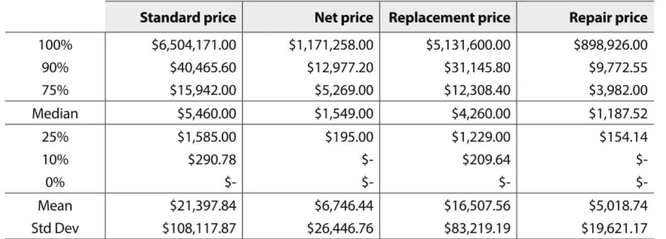
Numerous prices are associated with each item. Four price types correspond to the potential revenue and inventory replenishment costs. Standard price(P) rep-resents the worst-case scenario for the customer. If a customer is unable to return a carcass to the pipeline for possible repair and reissue, the standard price is charged for that order. On the other hand, if the cus-tomer is able to return the carcass, the net price(P_NET)

is charged. The incoming revenue for that order would be added back to the WSS inventory budget and used for further inventory replenishment. As WSS deter-mines what inventory to replenish, it must decide between repairing and replacing assets. The supplier charges WSS with either the repair price(P_R) attached to the asset, if it is repaired, or the replacement price (P_PROC), if it is a new procurement. Table 11 shows the respective summary statistics.

(10)

prices

Standard price Net price Replacement price Repair price

100% 90% 75%

$6,504,171.00 $40,465.60 $15,942.00

$1,171,258.00 $12,977.20 $5,269.00

$5,131,600.00 $31,145.80 $12,308.40

$898,926.00 $9,772.55 $3,982.00

Median $5,460.00 $1,549.00 $4,260.00 $1,187.52

25% 10% 0%

$1,585.00 $290.78

$-$195.00

$-$1,229.00 $209.64

$-$154.14 $-Mean

Std Dev

$21,397.84 $108,117.87

$6,746.44 $26,446.76

$16,507.56 $83,219.19

$5,018.74 $19,621.17

Final variable selection

Demand, reparability, lead times, criticality and price are primary fill rate drivers that affect WSS’s abil-ity to maximize equipment availabilabil-ity. Therefore, they must be present in any model used to prioritize items for resource allocation and management. We discussed 21 specific variables in this section as fill rate and equipment availability drivers, but we do not need to use all them to prioritize the items. They can be represented through various creative combinations and variable substitutions. We want to limit the num-ber of variables in the final analysis to maintain a par-simonious framework, while capturing as much of the important data as possible. We whittle our list down to six variables: criticality, demand value, number of requisitions, requisition variance, PPV, and PPV vari-ance. We now describe the logic behind these choices.

We first make a note about the period of interest. We include items with demand of at least 1 unit over a 36-month period ending in May of 2014. However, to compute each of the six variables of interest, we do not necessarily include information over that entire 36 months. For variables related to requisitions, requisi-tion variance, and high-priority requisirequisi-tions, we used data over a 24-month period. Whisky requisition data covers a range from April 2013 through March 2014. We chose the two-year requisition and one-year whisky requisition time frames because those time frames are most representative of future requirements.

Conceiv-ably, the item management processes would address any major supply issues prior to those time frames.

Number of requisitions (X) and requisition variance (σX2)

warrant their own individual model variables. Every requisition of an item affects fill rate the same way, regardless of criticality, price, or quantity. Requisition and requisition variance are the best tools to predict and plan for the volume and predictability of future requisitions. This proper planning then leads to req-uisition fulfillment and fill rate metrics.

To create one criticality variable, we incorporate high-priority requisitions over the past 24 months, whisky requisitions over the past 12 months, and the IMEC code. The formula used to calculate the criticality score is shown in equation (2).

K = 1.5 *W + H + 0.1 *IMEC*X (2)

The formulation is subjective in nature, but proves to be a good approximation of the importance of each measure to the overall criticality score. A requisition is often under more than one priority criteria (whisky, high-priority, and high IMEC), so it may contribute in three different ways to the item’s criticality score (K). In this formulation, whisky requisitions weigh 50% higher than high-priority requisitions, which may im-pact the items criticality more heavily than its IMEC code. Table 12 shows how criticality scores are calcu-lated for 12 different items.

Table 12. Criticality scores and rankings for 8 hypothetical items

item IMEC Requisitions (X) Whiskeys (W) Hi-Pri (H) Criticality (K)

1 4 2000 1173 891 3450

(11)

78 ARTICLES |Applying Inventory Classification to a Large Inventory Management System

ISSN: 1984-3046 © joSCM | São Paulo | V. 10 | n. 1 | jan-june 2017 | 68-86

3 3 2000 1093 912 3151

4 3 100 51 16 122

5 2 2000 122 100 683

6 2 100 43 34 118

7 1 2000 606 315 1424

8 1 100 18 12 49

We also include procurement problem variable (PPV)

and its variance

Procurement

100% 240.00 894.25 984.25 461.73

90% 1.64 6.30 7.39 3.35

75% 1.04 4.00 5.20 2.41

Median 1.04 2.83 3.97 1.74

25% 0.99 1.70 2.74 0.88

10% 0.82 0.70 1.74 0.00

0% 0.00 0.00 0.30 0.00

Mean 4.73 8.84 13.57 2.53

Std Dev 17.92 35.85 48.18 11.79

𝑃𝑃𝑃𝑃𝑃𝑃 = 𝐷𝐷 ∗ 𝐿𝐿𝑃𝑃𝑃𝑃𝑃𝑃𝐶𝐶∗ 𝜌𝜌𝐿𝐿𝑃𝑃𝐿𝐿𝐿𝐿+ 𝐷𝐷 ∗ 𝐿𝐿𝑃𝑃 ∗ (1 − 𝜌𝜌𝐿𝐿𝑃𝑃𝐿𝐿𝐿𝐿) (1) Table 7 provides the statistics for PPV and PPV variance (𝜎𝜎𝑃𝑃𝑃𝑃𝑃𝑃2 ). Once again, a small number of items is responsible for most cases of high PPV and high PPV variance values.

in the model. They reflect the potential pipeline problems associated with each item, by integrating attrition demand, regeneration demand, procurement lead time, repair pipeline loss rate, and repair turnaround time. PPV and PPV vari-ance are extremely important to fill rate goals because even if WSS knows exactly what the future demand is going to be, if the parts are not on the shelf due to pipeline issues, the requisition scores a “miss” and fill rate decreases.

There are several issues to consider when determining how to factor price into the model. Because WSS has more control over spending than it does over revenue, inventory cost proves to be the best basis for the mod-el’s demand value variable. In summary, the demand value(V) considers unit demand, repair pipeline loss rate, repair price, and replacement price to calculate an expected cost for WSS to supply that unit demand.

The formulation used for demand value is shown be-low in equation (3).

item 𝑰𝑰𝑰𝑰𝑰𝑰𝑰𝑰 ₍_𝑿𝑿₎ ₍_𝑾𝑾₎ ₍_𝑯𝑯₎ ₍_𝑲𝑲₎

1 4 2000 1173 891 3450

2 4 100 57 1 126

3 3 2000 1093 912 3151

4 3 100 51 16 122

5 2 2000 122 100 683

6 2 100 43 34 118

7 1 2000 606 315 1424

8 1 100 18 12 49

We also include procurement problem variable (𝑃𝑃𝑃𝑃𝑃𝑃) and its variance (𝜎𝜎𝑃𝑃𝑃𝑃𝑃𝑃2 ) in the model. They reflect the potential pipeline problems associated with each item, by integrating attrition demand, regeneration demand, procurement lead time, repair pipeline loss rate, and repair turnaround time. PPV and PPV variance are extremely important to fill rate goals because even if WSS knows exactly what the future demand is going to be, if the parts are not on the shelf due to pipeline issues, the requisition scores a “miss” and fill rate decreases.

There are several issues to consider when determining how to factor price into the model. Because WSS has more control over spending than it does over revenue, inventory cost proves to be the best basis for the model’s demand value variable. In summary, the demand value (𝑃𝑃) considers unit demand, repair pipeline loss rate, repair price, and replacement price to calculate an expected cost for WSS to supply that unit demand. The formulation used for demand value is shown below in equation (3).

𝑃𝑃 = 𝜌𝜌𝐿𝐿𝐿𝐿𝐿𝐿𝐿𝐿∗ 𝐷𝐷 ∗ 𝑃𝑃𝑃𝑃𝑃𝑃𝐿𝐿𝑃𝑃+ (1 − 𝜌𝜌𝐿𝐿𝐿𝐿𝐿𝐿𝐿𝐿) ∗ 𝐷𝐷 ∗ 𝑃𝑃𝑃𝑃 (3)

5 METHODOLOGY

We now turn to developing the machinery that will transform the values of the six variables from Table 13 into a score for each item. We can then prioritize them according to this score. Recalling the list of methods from Section 2, we focus on WLO, SCMC, and WNO as potential prioritization candidates. Because SCMC improves upon WLO, and WNO improves slightly upon SCMC, we start with WNO. To reiterate, the major benefits of the WNO model are the

(3)

METHODOLOGY

We now turn to developing the machinery that will transform the values of the six variables from Table 13 into a score for each item. We can then prioritize them according to this score. Recalling the list of methods from Section , we focus on WLO, SCMC, and WNO as potential prioritization candidates. Because SCMC improves upon WLO, and WNO improves slightly upon SCMC, we start with WNO. To reiter-ate, the major benefits of the WNO model are the abil-ity to run without specialized software, the abilabil-ity to consider any number of criteria, the priority ranking of variables, and the ability to rank items individually.

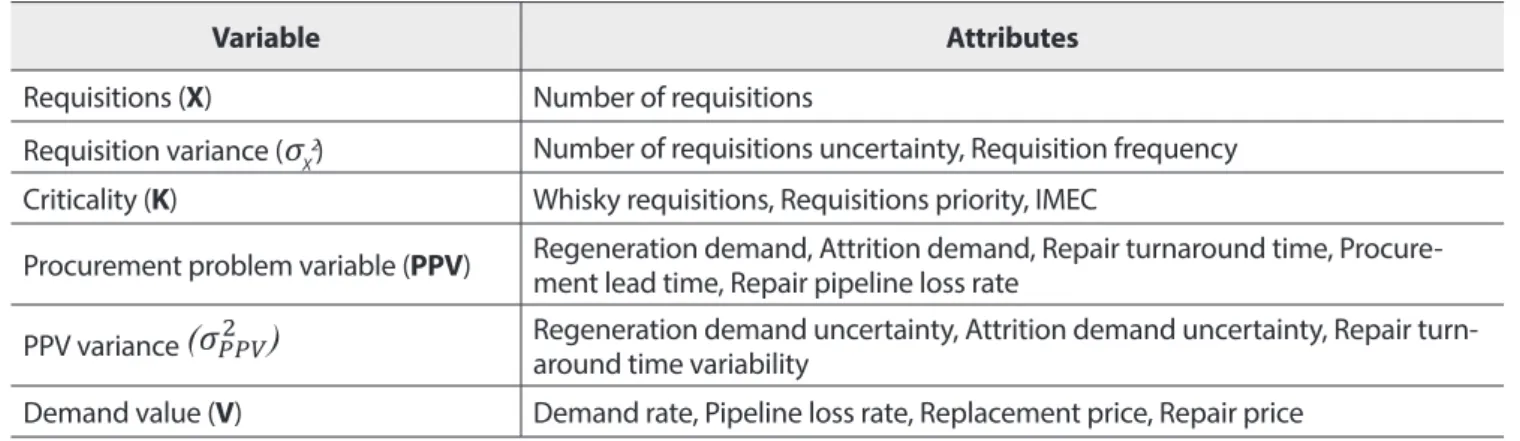
Table 13. Variables selected to prioritize items

Variable Attributes

Requisitions (X) Number of requisitions

Requisition variance (σ_X2₎ _{Number of requisitions uncertainty, Requisition frequency}

Criticality (K) Whisky requisitions, Requisitions priority, IMEC

Procurement problem variable (PPV) Regeneration demand, Attrition demand, Repair turnaround time, Procure-_{ment lead time, Repair pipeline loss rate} PPV variance

Procurement

100% 240.00 894.25 984.25 461.73

90% 1.64 6.30 7.39 3.35

75% 1.04 4.00 5.20 2.41

Median 1.04 2.83 3.97 1.74

25% 0.99 1.70 2.74 0.88

10% 0.82 0.70 1.74 0.00

0% 0.00 0.00 0.30 0.00

Mean 4.73 8.84 13.57 2.53

Std Dev 17.92 35.85 48.18 11.79

𝑃𝑃𝑃𝑃𝑃𝑃 = 𝐷𝐷 ∗ 𝐿𝐿𝑃𝑃𝑃𝑃𝑃𝑃𝐶𝐶∗ 𝜌𝜌𝐿𝐿𝑃𝑃𝐿𝐿𝐿𝐿+ 𝐷𝐷 ∗ 𝐿𝐿𝑃𝑃∗ (1 − 𝜌𝜌𝐿𝐿𝑃𝑃𝐿𝐿𝐿𝐿) (1) Table 7 provides the statistics for PPV and PPV variance (𝜎𝜎𝑃𝑃𝑃𝑃𝑃𝑃2 ). Once again, a small number of items is responsible for most cases of high PPV and high PPV variance values.

Regeneration demand uncertainty, Attrition demand uncertainty, Repair turn-around time variability

Demand value (V) Demand rate, Pipeline loss rate, Replacement price, Repair price

The inputs for the WNO model are the relevant vari-ables associated with each item and the subjective priority ranking of all variables established by the de-cision maker. We label the variables in ascending or-der according to the priority specified by the decision maker. Next, each item is scored for every variable ac-cording to its relative ranking among all items. If the value of the jth_{variable for the}_ith_{item is , then this}

item’s score according to the jth_{variable is , the result}

of the following expression (Ng 2007, Hadi-Vencheh 2010):

ability to run without specialized software, the ability to consider any number of criteria, the priority ranking of variables, and the ability to rank items individually.

Table 13. Variables selected to prioritize items

Requisitions (𝑿𝑿) Number of requisitions

Requisition variance (𝝈𝝈𝑿𝑿𝟐𝟐) Number of requisitions uncertainty, Requisition frequency Criticality (𝑲𝑲) Whisky requisitions, Requisitions priority, IMEC

Procurement problem variable (𝑷𝑷𝑷𝑷𝑷𝑷)

Regeneration demand, Attrition demand, Repair turnaround time, Procurement lead time, Repair pipeline loss rate

PPV variance (𝝈𝝈𝑷𝑷𝑷𝑷𝑷𝑷𝟐𝟐 ) Regeneration demand uncertainty, Attrition demand uncertainty, _{Repair turnaround time variability} Demand value (𝑷𝑷) Demand rate, Pipeline loss rate, Replacement price, Repair price

The inputs for the WNO model are the relevant variables associated with each item and the subjective priority ranking of all variables established by the decision maker. We label the variables in ascending order according to the priority specified by the decision maker. Next, each item is scored for every variable according to its relative ranking among all items. If the value of the jth_{variable for the}_ith_{item is}_𝑦𝑦

𝑖𝑖𝑖𝑖, then this item’s score according to the jth variable is

𝛼𝛼𝑖𝑖𝑖𝑖, the result of the following expression (Ng 2007, Hadi-Vencheh 2010):

𝛼𝛼𝑖𝑖𝑖𝑖 = _max 𝑦𝑦𝑖𝑖𝑖𝑖−min𝑖𝑖=1,2,…𝐼𝐼{𝑦𝑦𝑖𝑖𝑖𝑖} 𝑖𝑖=1,2,…𝐼𝐼{𝑦𝑦𝑖𝑖𝑖𝑖}−min𝑖𝑖−1,2,…𝐼𝐼{𝑦𝑦𝑖𝑖𝑖𝑖}

Considering the relative importance of each variable, an optimization specifies their weights by maximizing the weighted sum of the scores obtained by each item:

max𝑤𝑤𝑖𝑖∑ 𝑤𝑤𝐽𝐽𝑖𝑖 𝑖𝑖∑𝐼𝐼𝑖𝑖=1𝛼𝛼𝑖𝑖𝑖𝑖 (4)

subject to ∑𝐽𝐽𝑖𝑖=1𝑤𝑤𝑖𝑖2 = 1

𝑤𝑤𝑖𝑖 ≥ 𝑤𝑤𝑖𝑖+1 ≥ 0, 𝑗𝑗 = 1,2, … , 𝐽𝐽 − 1

The objective function (4) intends to find the array of weights that maximizes the sum of final scores subject to the following constraints: the sum of the squared weights equals to 1, as

(12)

79 AUTHORS | Benjamin Isaac May | Michael P. Atkinson | Geraldo Ferrer

Requisition variance (𝝈𝝈𝑿𝑿𝟐𝟐) Number of requisitions uncertainty, Requisition frequency

Criticality (𝑲𝑲) Whisky requisitions, Requisitions priority, IMEC Procurement problem

variable (𝑷𝑷𝑷𝑷𝑷𝑷)

PPV variance (𝝈𝝈𝑷𝑷𝑷𝑷𝑷𝑷𝟐𝟐 ) Regeneration demand uncertainty, Attrition demand uncertainty, _{Repair turnaround time variability}

Demand value (𝑷𝑷) Demand rate, Pipeline loss rate, Replacement price, Repair price

𝛼𝛼𝑖𝑖𝑖𝑖=_max 𝑦𝑦𝑖𝑖𝑖𝑖−min𝑖𝑖=1,2,…𝐼𝐼{𝑦𝑦𝑖𝑖𝑖𝑖}

𝑖𝑖=1,2,…𝐼𝐼{𝑦𝑦𝑖𝑖𝑖𝑖}−min𝑖𝑖−1,2,…𝐼𝐼{𝑦𝑦𝑖𝑖𝑖𝑖}

max𝑤𝑤_𝑖𝑖∑ 𝑤𝑤𝐽𝐽𝑖𝑖 𝑖𝑖∑𝐼𝐼𝑖𝑖=1𝛼𝛼𝑖𝑖𝑖𝑖 (4)

subject to ∑𝐽𝐽𝑖𝑖=1𝑤𝑤𝑖𝑖2= 1

𝑤𝑤𝑖𝑖≥ 𝑤𝑤𝑖𝑖+1≥ 0, 𝑗𝑗 = 1,2, … , 𝐽𝐽 − 1

The objective function (4) intends to find the array of weights that maximizes the sum of final scores subject to the following constraints: the sum of the squared weights equals to 1, as recommended by Hadi-Vencheh, and the weights are monotonically increasing, according to the

variable (𝑷𝑷𝑷𝑷𝑷𝑷)

PPV variance (𝝈𝝈𝑷𝑷𝑷𝑷𝑷𝑷𝟐𝟐 ) Regeneration demand uncertainty, Attrition demand uncertainty, _{Repair turnaround time variability}

𝛼𝛼𝑖𝑖𝑖𝑖=_max_{𝑖𝑖=1,2,…𝐼𝐼}𝑦𝑦𝑖𝑖𝑖𝑖−min_{𝑦𝑦_{𝑖𝑖𝑖𝑖}𝑖𝑖=1,2,…𝐼𝐼_}−min_{𝑖𝑖−1,2,…𝐼𝐼}{𝑦𝑦𝑖𝑖𝑖𝑖} _{𝑦𝑦_{𝑖𝑖𝑖𝑖}_}

max𝑤𝑤𝑖𝑖∑ 𝑤𝑤𝐽𝐽𝑖𝑖 𝑖𝑖∑𝐼𝐼𝑖𝑖=1𝛼𝛼𝑖𝑖𝑖𝑖 (4)

𝑤𝑤𝑖𝑖≥ 𝑤𝑤𝑖𝑖+1≥ 0, 𝑗𝑗 = 1,2, … , 𝐽𝐽 − 1

The objective function (4) intends to find the array of weights that maximizes the sum of final scores subject to the following constraints: the sum of the squared weights equals to 1, as recommended by Hadi-Vencheh, and the weights are monotonically increasing, according to the priority ranking of variables, and the ability to rank items individually.

variable (𝑷𝑷𝑷𝑷𝑷𝑷) Regeneration demand, Attrition demand, Repair turnaround time, Procurement lead time, Repair pipeline loss rate PPV variance (𝝈𝝈𝑷𝑷𝑷𝑷𝑷𝑷𝟐𝟐 ) Regeneration demand uncertainty, Attrition demand uncertainty, _{Repair turnaround time variability}

𝛼𝛼𝑖𝑖𝑖𝑖=_max_{𝑖𝑖=1,2,…𝐼𝐼}𝑦𝑦𝑖𝑖𝑖𝑖−min_{𝑦𝑦_{𝑖𝑖𝑖𝑖}𝑖𝑖=1,2,…𝐼𝐼_}−min_{𝑖𝑖−1,2,…𝐼𝐼}{𝑦𝑦𝑖𝑖𝑖𝑖} _{𝑦𝑦_{𝑖𝑖𝑖𝑖}_}

max𝑤𝑤𝑖𝑖∑ 𝑤𝑤𝑖𝑖∑𝐼𝐼𝑖𝑖=1𝛼𝛼𝑖𝑖𝑖𝑖 𝐽𝐽

𝑖𝑖 (4)

𝑤𝑤𝑖𝑖≥ 𝑤𝑤𝑖𝑖+1≥ 0, 𝑗𝑗 = 1,2, … , 𝐽𝐽 − 1

The objective function (4) intends to find the array of weights that maximizes the sum of final scores subject to the following constraints: the sum of the squared weights equals to 1, as recommended by Hadi-Vencheh, and the weights are monotonically increasing, according to the

The objective function (4) intends to find the array of weights that maximizes the sum of final scores subject to the following constraints: the sum of the squared weights equals to 1, as recommended by Hadi-Vencheh, and the weights are monotonically increasing, according to the subjective ranking previ-ously determined by the decision maker. By squaring the weights, we avoid results that assign the value of zero to some weights, an important consideration to ensure that all variables are represented in the priori-tization scheme.

Our objective function is modified from the origi-nal WNO model proposed by Hadi-Vencheh. In that model, the user solves a separate optimization model for each item, rather than a single optimization over the sum of scores for each variable. Our simplification allows easy integration with ERP systems, an impor-tant concern if you have a large number of stock-keep-ing units or a large number of variables

In order to perform the optimization in (4), we must rank the selected variables

subjective ranking previously determined by the decision maker. By squaring the weights, we avoid results that assign the value of zero to some weights, an important consideration to ensure that all variables are represented in the prioritization scheme.

Our objective function is modified from the original WNO model proposed by Hadi -Vencheh. In that model, the user solves a separate optimization model for each item, rather than a single optimization over the sum of scores for each variable. Our simplification allows easy integration with ERP systems, an important concern if you have a large number of stock-keeping units or a large number of variables

In order to perform the optimization in (4), we must rank the selected variables

(𝑋𝑋, 𝜎𝜎𝑋𝑋2, 𝐾𝐾, 𝑃𝑃𝑃𝑃𝑃𝑃, 𝜎𝜎𝑃𝑃𝑃𝑃𝑃𝑃2 , 𝑃𝑃) in order of importance. In addition to choice of time frame for data

selection, this is the only subjective part of the model. All six variables include some measure of demand rate. Therefore, number of requisitions (𝑋𝑋) is strongly represented regardless of the variable ranking. With that in mind, focus shifts to variables that encompass other aspects affecting equipment availability.

Criticality (𝐾𝐾) represents equipment availability better than all other variables. The fact that just one small part could potentially render an entire warship not operationally ready is reason enough to designate criticality as the highest priority variable. Demand value (𝑃𝑃) falls in line with the original theory behind ABC analysis. Resources committed to stagnant inventory severely diminish a business’s ability to fund high-demand and/or highly critical stock. Stagnant stock not only limits replenishment of high-demand stock that drives fill rate, but also critical parts that strongly affect equipment availability. We assign demand value as the second highest priority variable to capture WSS’s need to be efficient with its limited budget.

in order of importance. In addition to choice of time frame for data selection, this is the only subjective part of the model. All six variables include some measure of demand rate. Therefore, number of requisitions (X) is strongly represented regardless of the variable ranking. With that in mind, focus shifts to variables that encompass other aspects affecting equipment availability.

Criticality (K) represents equipment availability better than all other variables. The fact that just one small part could potentially render an entire warship not operationally ready is reason enough to designate criti-cality as the highest priority variable. Demand value (V) falls in line with the original theory behind ABC analysis. Resources committed to stagnant inventory severely diminish a business’s ability to fund high-de-mand and/or highly critical stock. Stagnant stock not only limits replenishment of high-demand stock that drives fill rate, but also critical parts that strongly affect equipment availability. We assign demand value as the second highest priority variable to capture WSS’s need to be efficient with its limited budget.

Figure 2: WNO structure with selected variables

Figure 2: WNO structure with selected variables

Requisitions, requisition variance, procurement problem variable, and PPV variance are all heavily correlated with demand. Though PPV and PPV variance can identify potential pipeline problems created by long lead-times, high values aren’t necessarily indicative of greater concerns. If inventory levels are set high enough for a high-PPV item, the pipeline may still be healthy. Still, the item does have the potential to quickly experience major issues due to demand or lead time volatility. On the other hand, high requisitions and requisition variance values do

Requisitions, requisition variance, procurement prob-lem variable, and PPV variance are all heavily correlat-ed with demand. Though PPV and PPV variance can identify potential pipeline problems created by long lead-times, high values aren’t necessarily indicative of greater concerns. If inventory levels are set high enough for a high-PPV item, the pipeline may still be healthy. Still, the item does have the potential to quickly experience major issues due to demand or lead time volatility. On the other hand, high requisitions and requisition variance values do directly reflect higher importance to fill rate and equipment availabil-ity. Therefore, we ranked the remaining four variables in this order: number of requisitions (X), requisition variance (σX2), procurement problem variable (PPV)

and PPV variance

Procurement

100% 240.00 894.25 984.25 461.73

90% 1.64 6.30 7.39 3.35

75% 1.04 4.00 5.20 2.41

Median 1.04 2.83 3.97 1.74

25% 0.99 1.70 2.74 0.88

10% 0.82 0.70 1.74 0.00

0% 0.00 0.00 0.30 0.00

Mean 4.73 8.84 13.57 2.53

Std Dev 17.92 35.85 48.18 11.79

(13)

variables in the raw data participate in the variables selected in the model to build each item’s score.

MODEL ANALYSIS

One of the major advantages of the modified WNO model is its simplicity. The input of the classifica-tion scheme is the set of weights associated with each variable in the objective function in section . To generate a score, we compute the weighted sum of the standardized variables associated with that item. The weighted sum of all criteria (A_i) becomes the final score for the ith_{item used in the priority scheme.}

procurement problem variable (𝑃𝑃𝑃𝑃𝑃𝑃) and PPV variance (𝜎𝜎𝑃𝑃𝑃𝑃𝑃𝑃2 ). Figure 2 shows how the

variables in the raw data participate in the variables selected in the model to build each item’s score.

6 MODEL ANALYSIS

One of the major advantages of the modified WNO model is its simplicity. The input of the classification scheme is the set of weights associated with each variable in the objective function in section 5. To generate a score, we compute the weighted sum of the standardized variables associated with that item. The weighted sum of all criteria (𝐴𝐴_𝑖𝑖) becomes the final score for the ith item used in the priority scheme.

𝐴𝐴𝑖𝑖 = ∑ 𝑤𝑤𝐽𝐽𝑗𝑗 𝑗𝑗∗ 𝛼𝛼𝑖𝑖𝑗𝑗 (5)

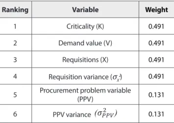
We then prioritize items by their individual scores. Table 14 presents the optimal weights for our WSS data. To generate the numbers in this table we find the coefficients 𝑤𝑤𝑗𝑗 by solving

the objective function in equation (4) using the Generalized Reduced Gradient (GRG) non-linear optimization algorithm available in the Solver add-in in MS Excel 2014 on a MacBook Pro 2.7 GHz. We specified a multi-start method with a population size of 250 random starting points, where each starting point was a different weight array.

Table 14. Optimal weights for the WNO model

Ranking Variable Weight

1 Criticality (𝐾𝐾) 0.491

2 Demand value (𝑃𝑃) 0.491

3 Requisitions (𝑋𝑋) 0.491

4 Requisition variance (𝜎𝜎𝑋𝑋2) 0.491

5 Procurement problem variable (𝑃𝑃𝑃𝑃𝑃𝑃) 0.131

6 PPV variance (𝜎𝜎𝑃𝑃𝑃𝑃𝑃𝑃2 ) 0.131

Recall that the WNO model constrains the sum of squared weights to 1 and that the weights must have non-increasing values according to the variable prioritization described

(5)

We then prioritize items by their individual scores. Table 14 presents the optimal weights for our WSS data. To generate the numbers in this table we find the coefficients w_j by solving the objective function in equation (4) using the Generalized Reduced Gradient (GRG) non-linear optimization algorithm available in the Solver add-in in MS Excel 2014 on a MacBook Pro 2.7 GHz. We specified a multi-start method with a population size of 250 random starting points, where each starting point was a different weight array.

Table 14. Optimal weights for the WNO model

Ranking Variable Weight

1 Criticality (K) 0.491

2 Demand value (V) 0.491

3 Requisitions (X) 0.491

4 Requisition variance (σ_X2₎ _0.491

5 Procurement problem variable _(PPV) 0.131

6 PPV variance

Procurement

100% 240.00 894.25 984.25 461.73

90% 1.64 6.30 7.39 3.35

75% 1.04 4.00 5.20 2.41

Median 1.04 2.83 3.97 1.74

25% 0.99 1.70 2.74 0.88

10% 0.82 0.70 1.74 0.00

0% 0.00 0.00 0.30 0.00

Mean 4.73 8.84 13.57 2.53

Std Dev 17.92 35.85 48.18 11.79

𝑃𝑃𝑃𝑃𝑃𝑃 = 𝐷𝐷 ∗ 𝐿𝐿𝑃𝑃𝑃𝑃𝑃𝑃𝐶𝐶∗ 𝜌𝜌𝐿𝐿𝑃𝑃𝐿𝐿𝐿𝐿+ 𝐷𝐷 ∗ 𝐿𝐿𝑃𝑃 ∗ (1 − 𝜌𝜌𝐿𝐿𝑃𝑃𝐿𝐿𝐿𝐿) (1) Table 7 provides the statistics for PPV and PPV variance (𝜎𝜎𝑃𝑃𝑃𝑃𝑃𝑃2 ). Once again, a small number of items is responsible for most cases of high PPV and high PPV variance values.

0.131

Recall that the WNO model constrains the sum of squared weights to 1 and that the weights must have non-increasing values according to the variable pri-oritization described above. In this case, WNO as-signs criticality, demand value, requisitions, and requisition variance an equal weight. Based on the priority constraint, this suggests that the requisition variables are particularly crucial attributes. If the maximization were unconstrained, requisition vari-ance would receive the highest weight.

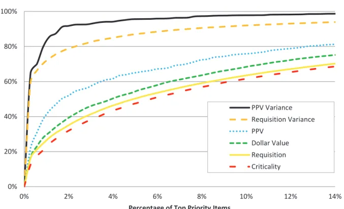
Given the optimal weights, we can score each item and evaluate our priority scheme against a few can-didate prioritizations. To do this we focus on the Pa-reto nature of the original ABC analysis: if the WNO rankings are effective, a small fraction of the top ranked items (the “A” items) should capture a large fraction of the key business drivers. In the follow-ing section we create a Pareto plot to examine if the highest ranked items according to the WNO method capture a large fraction of requisitions, PPV, critical-ity and demand value.

WNO results

Figure 3 is a Pareto chart that shows the increasing amount of the six selected variables that are captured by the WNO model. Starting with the highest ranked item, it successively adds the highest ranked among the ones still remaining, one by one, as desired. Each curve refers to a single variable in the model. The x-axis represents the percentage of all 17,857 items ranked according to WNO. The y-axis represents the cumulative percentage of the variable captured by those items. The chart shows that PPV variance in the 17,857 items (black continuous line) is quickly cap-tured by the first few items: just 2% of the items (351 items) ranked by WNO capture 92% of the PPV vari-ance in the data. These same items also capture 79% of the requisition variance (long dashed line), 52% of the procurement problem variable (light dotted line), 39% of demand value (short dashed line), 35% of all requisitions (light continuous line) and 32% of the criticality (dot-dashed line) present in our dataset. Figure 3 illustrates the Pareto shape that we desire. A few items account for a large fraction of the metrics of interest. For all 6 metrics, 10% of the highest ranked items capture at least 60% of each variable identified as the key business drivers in the organization.

The approach adopted by this organization, the WSS4 method, categorizes 673 items as A. If we se-lect the top 673 items of the WNO ranking (3.8% of the total), they capture 94%, 84.6%, 61.2%, 49.5%, 45.6%, and 42.6% of the data’s total PPV variance, requisition variance, PPV, demand value, number of requisitions, and criticality, respectively.