Available online throug
ISSN 2229 – 5046
EFFECT OF HALL CURRENTS, THERMOPHORESIS ON THE MHD MIXED CONVECTIVE
FLOW PAST A PERMEABLE STRETCHING SURFACE WITH THERMAL RADIATION
KALYANI Ch
1, SREELAKSHMI K
2AND SAROJAMMA G
3,*1, 2, 3
Department of Applied Mathematics,
Sri Padmavati Mahila Visvavidyalayam, Tirupati-517502, India.
(Received On: 04-04-16; Revised & Accepted On: 17-04-16)
ABSTRACT
T
he present analysis deals with the effect of Hall currents, thermal radiation on the mixed convection flow of a viscousincompressible electrically conducting fluid past an unsteady porous stretching sheet embedded in a porous medium under the influence of transverse uniform magnetic field in the presence of thermophoresis and chemical reaction with convective boundary condition. Numerical solutions of the governing equations are obtained using Keller-box technique. The profiles of primary and secondary velocities, temperature and concentration are graphically presented for various values of suction parameter, thermal radiation parameter, Hall parameter, magnetic parameter etc. The values of local skin friction coefficient, local Nusselt number and local Sherwood number are tabulated for various values of parameters that occur in the analysis.
Keywords: MHD, Hall currents, convective boundary condition, thermophoresis.
1. INTRODUCTION
Thermophoresis is a phenomenon in which micro-sized particles, when suspended in a gas with thermal gradient, experience a force which causes the small particles to move from a hot surface towards a colder one. The force experienced by these particles as a result of the temperature gradient is known as thermophoretic force and the velocity with which the particles move is called the thermophoretic velocity. Thermophoresis is found to be one of the important mechanisms of mass transfer in the process of modified chemical vapor deposition (MCVD). This phenomenon plays a significant role in a wide range of applications such as the production of ceramic powders in high temperature aerosol flow reactors and optical fibers obtained by the MCVD process. It is observed that the thermophoretic deposition of the radioactive particles to be one of the reasons for the occurrence of accidents in the nuclear reactors. The principle of thermophoresis is employed in the manufacturing of graded index silicon dioxide and germanium dioxide optical fiber. Goldsmith and May (1966) appear to be the first researchers to investigate the thermophoretic transport in a one-dimensional flow to measure the thermophoretic velocity. Hales et al. (1972) studied the thermophoretic deposition of the aerosol particles on to an isothermal vertical surface situated adjacent to a large body of an otherwise quiescent air- stream-aerosol mixture. Selim et al. (2003) studied the effects of thermophoresis and non uniform surface mass flux on the mixed convection flow past a heated vertical permeable plate.
Thermal radiation plays a vital role in manufacturing process in industry. For example, in casting and levitation, metallic rolling, design of furnace and fins etc. In engineering, many processes involve very high temperatures and the application of radiative heat transfer is essentially required to design the specific equipment. Nuclear power plants, gas turbines, satellites and space vehicles are some of the examples (Seddeek (2002)) which involve radiative heat transfer.
In this paper we made an effort to study the effects of Hall currents, thermophoresis and heat source/sink on the unsteady flow of a viscous incompressible electrically conducting fluid past a porous stretching sheet embedded in a porous medium subject to a transverse magnetic field in the presence of first order chemical reaction with velocity slip and convective heat boundary conditions.
2. MATHEMATICAL FORMULATION
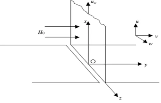
Consider the unsteady flow, heat and mass transfer of a viscous, incompressible and electrically conducting fluid past a vertical permeable stretching sheet coinciding with the plane 𝑦𝑦 = 0 and the flow is confined to the region 𝑦𝑦 > 0. A schematic representation of the physical model is shown in Fig. 1.
Fig. 1: Physical model and coordinate system
We choose the frame of reference (x, y, z) such that the x-axis is along the direction of motion of the surface, the y-axis is normal to the surface and the z-axis transverse to the xy-plane. An external constant magnetic field H0 is applied in the positive y-direction. The effects of thermophoresis, thermal radiation and chemical reaction are considered.
Taking Hall effects into consideration and assuming that the electron pressure gradient, the ion slip and the thermo-electric effects are negligible, the generalized Ohm's law can be written as (Sutton and Sherman (1965))
𝒋𝒋=𝜎𝜎 �𝑬𝑬+𝜇𝜇𝑒𝑒𝒒𝒒 ×𝑯𝑯 −𝑒𝑒𝑛𝑛𝜇𝜇𝑒𝑒𝑒𝑒𝒋𝒋×𝑯𝑯� (1)
where neand e stand for the electron number density and the electric charge, respectively, 𝜎𝜎(𝜎𝜎=𝑒𝑒2𝑛𝑛𝑒𝑒𝑇𝑇𝑒𝑒
𝑚𝑚𝑒𝑒 ) is the electrical conductivity, 𝑇𝑇𝑒𝑒 and 𝑚𝑚𝑒𝑒 denote the electron collision time and the mass of an electron respectively. The effect of Hall current gives rise to a force in the z-direction resulting in a cross-flow in this direction and thus the cross-flow becomes three-dimensional. where (u, v, w), (𝐸𝐸𝑥𝑥,𝐸𝐸𝑦𝑦,𝐸𝐸𝑧𝑧) and ( 𝑗𝑗𝑥𝑥,𝑗𝑗𝑦𝑦,𝑗𝑗𝑧𝑧) are the components of 𝒒𝒒, E and j respectively. In this study, we assume that the magnetic Reynolds number is small
(𝑅𝑅𝑒𝑒𝑚𝑚≪1) so that the induced magnetic field is negligible. 𝑗𝑗𝑦𝑦is a constant due to the equation of conservation of electric charge 𝛻𝛻.𝒋𝒋= 0. Since 𝑗𝑗𝑦𝑦 = 0 at the plate which is electrically non-conducting, we obtain 𝑗𝑗𝑦𝑦 = 0 everywhere in the flow.
Hence (1) reduces to
𝐽𝐽𝑥𝑥=(1+𝜎𝜎𝜎𝜎𝑚𝑚2)(𝑚𝑚𝑚𝑚 − 𝑤𝑤) (2) 𝐽𝐽𝑧𝑧 =(1+𝜎𝜎𝜎𝜎𝑚𝑚2)(𝑚𝑚+𝑚𝑚𝑤𝑤) (3)
where (u, v, w) are the velocity components in the (x, y, z) directions respectively, m (=𝜔𝜔𝑒𝑒𝑡𝑡𝑒𝑒) is the Hall parameter,
𝜎𝜎=𝜇𝜇𝑒𝑒𝐻𝐻0is the strength of the imposed magnetic field and 𝜔𝜔𝑒𝑒 is the electron frequency.
The continuity, momentum, energy and concentration equations governing such type of flow can be written as 𝜕𝜕𝑚𝑚
𝜕𝜕𝑥𝑥 +
𝜕𝜕𝜕𝜕
𝜕𝜕𝑦𝑦 = 0 (4)
𝜕𝜕𝑚𝑚 𝜕𝜕𝑡𝑡 +𝑚𝑚
𝜕𝜕𝑚𝑚 𝜕𝜕𝑥𝑥 +𝜕𝜕
𝜕𝜕𝑚𝑚
𝜕𝜕𝑦𝑦 = 𝜈𝜈
𝜕𝜕2𝑚𝑚 𝜕𝜕𝑦𝑦2 − 𝜎𝜎𝜎𝜎
2
𝜕𝜕𝑤𝑤
𝜕𝜕𝑡𝑡 +𝑚𝑚 𝜕𝜕𝑤𝑤 𝜕𝜕𝑥𝑥 +𝜕𝜕
𝜕𝜕𝑤𝑤 𝜕𝜕𝑦𝑦 =𝜈𝜈
𝜕𝜕2𝑤𝑤
𝜕𝜕𝑦𝑦2 +
𝜎𝜎𝜎𝜎2
𝜌𝜌(1+𝑚𝑚2)(𝑚𝑚𝑚𝑚 − 𝑤𝑤)−
𝜈𝜈
𝑘𝑘1𝑤𝑤 (6)
𝜕𝜕𝑇𝑇 𝜕𝜕𝑡𝑡 +𝑚𝑚
𝜕𝜕𝑇𝑇 𝜕𝜕𝑥𝑥 +𝜕𝜕
𝜕𝜕𝑇𝑇 𝜕𝜕𝑦𝑦 =
𝐾𝐾 𝜌𝜌𝑐𝑐𝑝𝑝
𝜕𝜕2𝑇𝑇
𝜕𝜕𝑦𝑦2−𝜌𝜌𝑐𝑐𝑝𝑝1 𝜕𝜕𝑞𝑞𝑟𝑟𝜕𝜕𝑦𝑦 + 𝑄𝑄
∗
𝜌𝜌𝑐𝑐𝑝𝑝(𝑇𝑇 − 𝑇𝑇∞) (7) 𝜕𝜕𝜕𝜕
𝜕𝜕𝑡𝑡 +𝑚𝑚 𝜕𝜕𝜕𝜕 𝜕𝜕𝑥𝑥 +𝜕𝜕
𝜕𝜕𝜕𝜕 𝜕𝜕𝑦𝑦 =𝐷𝐷
𝜕𝜕2𝜕𝜕
𝜕𝜕𝑦𝑦2− 𝑘𝑘(𝜕𝜕 − 𝜕𝜕∞)−
𝜕𝜕
𝜕𝜕𝑦𝑦[𝑉𝑉𝑇𝑇(𝜕𝜕 − 𝜕𝜕∞)] (8)
Where T is the temperature inside the boundary layer, 𝑇𝑇∞ is the ambient temperature, C is the fluid concentration, 𝜕𝜕∞ is the ambient concentration, 𝛼𝛼 is thermal diffusivity, 𝜈𝜈 is the kinematic viscosity, 𝜌𝜌 is the density of the fluid, 𝜎𝜎 is the electrical conductivity, 𝑐𝑐𝑝𝑝 is the specific heat at constant pressure, μis the dynamic viscocity of the fluid, 𝑞𝑞𝑟𝑟 is the radiative heat flux, K is the thermal conductivity of the medium, k1 is the permeability of porous medium, D is the mass diffusivity, 𝑄𝑄∗ is the uniform volumetric heat absorption, k is the chemical reaction, 𝑉𝑉𝑇𝑇 is the thermophoresis velocity, following Talbot et al. (1980) taken as 𝑉𝑉𝑇𝑇 =− 𝑘𝑘𝑡𝑡𝜈𝜈
𝑇𝑇𝑟𝑟𝑒𝑒𝑟𝑟 𝜕𝜕𝑇𝑇
𝜕𝜕𝑦𝑦, where 𝑇𝑇𝑟𝑟𝑒𝑒𝑟𝑟 is some reference temperature, the value of 𝑘𝑘𝑡𝑡𝜈𝜈 represents the thermophoretic diffusivity.
By using Rosseland approximation, the radiative heat flux is given by
𝑞𝑞𝑟𝑟 = −4𝜎𝜎 ∗
3𝑘𝑘∗𝜕𝜕𝑇𝑇
4
𝜕𝜕𝑦𝑦 (9) Where 𝜎𝜎∗ is the Stefen-Boltzman constant and 𝑘𝑘∗ is the absorption coefficient.
𝑇𝑇4 may be linearly expanded in a Taylor’s series about 𝑇𝑇
∞ to get
𝑇𝑇4=𝑇𝑇
∞4+ 4𝑇𝑇∞3(𝑇𝑇 − 𝑇𝑇∞) + 6𝑇𝑇∞2(𝑇𝑇 − 𝑇𝑇∞)2+⋯, (10) and neglecting higher order terns beyond the first degree in (𝑇𝑇 − 𝑇𝑇∞),
we obtain 𝑇𝑇4≅4𝑇𝑇∞3𝑇𝑇 −3𝑇𝑇∞4 (11)
The boundary conditions of the problem are
u =𝑈𝑈𝑤𝑤+𝑁𝑁1𝜈𝜈𝜕𝜕𝑚𝑚
𝜕𝜕𝑦𝑦, v = −𝑉𝑉𝑤𝑤(x, t), w =𝑁𝑁1𝜈𝜈 𝜕𝜕𝑤𝑤 𝜕𝜕𝑦𝑦, −𝐾𝐾
𝜕𝜕𝑇𝑇
𝜕𝜕𝑦𝑦=ℎ𝑟𝑟(𝑇𝑇𝑟𝑟− 𝑇𝑇), C =𝜕𝜕𝑤𝑤(x, t) at y = 0, (12)
u→0, w→0, T→ 𝑇𝑇∞, C→ 𝜕𝜕∞ as y→ ∞ (13) where 𝑉𝑉𝑤𝑤(𝑥𝑥,𝑡𝑡) = (𝜈𝜈𝑈𝑈𝑤𝑤/𝑥𝑥)1 2⁄ 𝑟𝑟𝑤𝑤 represents the mass transfer at the surface with 𝑉𝑉𝑤𝑤 > 0 for injection and 𝑉𝑉𝑤𝑤 < 0 for suction, 𝑁𝑁1=𝑁𝑁0(1− 𝑐𝑐𝑡𝑡)1 2⁄ is the velocity slip factor which changes with time, 𝑁𝑁0 is the initial value of the velocity slip factor (at 𝑁𝑁1= 0, the no-slip case is observed), ℎ𝑟𝑟 is the convective heat transfer coefficient and 𝑇𝑇𝑟𝑟 is the convective fluid temperature.
The flow is induced by the stretching of the sheet which moves in its own plane with the surface velocity
𝑈𝑈𝑤𝑤(𝑥𝑥,𝑡𝑡) =(1𝑎𝑎𝑥𝑥−𝑐𝑐𝑡𝑡), where a (stretching rate) and c are the positive constants having dimension time−1 (with𝑐𝑐𝑡𝑡< 1,
𝑐𝑐 ≥0). It is noted that the stretching rate 𝑎𝑎
(1−𝑐𝑐𝑡𝑡)increases with time since a > 0.
The convective fluid temperature of the sheet varies with square of distance x from the slot and time t in the form
𝑇𝑇𝑟𝑟(𝑥𝑥,𝑡𝑡) =𝑇𝑇∞+ 𝑎𝑎𝑥𝑥
2
2𝜈𝜈(1−𝑐𝑐𝑡𝑡)3 2⁄ (14)
The surface concentration of the sheet varies with square of distance x from the slot and time t in the form
𝜕𝜕𝑤𝑤(𝑥𝑥,𝑡𝑡) =𝜕𝜕∞+ 𝑎𝑎𝑥𝑥
2
2𝜈𝜈(1−𝑐𝑐𝑡𝑡)3 2⁄ (15) where a is constant with𝑎𝑎 ≥0. It should be noted that when t = 0 (initial condition), equations (5) – (8) describe the case of steady flow over a stretching sheet. The particular form of 𝑈𝑈𝑤𝑤(𝑥𝑥,𝑡𝑡), 𝑇𝑇𝑟𝑟(𝑥𝑥,𝑡𝑡) and 𝜕𝜕𝑤𝑤(𝑥𝑥,𝑡𝑡) has been chosen in order to devise a similarity transformation which transforms the governing partial differential equations (5) – (8) into a set of highly nonlinear ordinary differential equations.
The stream function 𝜓𝜓(𝑥𝑥,𝑦𝑦,𝑡𝑡) is defined as:
𝑚𝑚=𝜕𝜕𝜓𝜓𝜕𝜕𝑦𝑦 =(1𝑎𝑎𝑥𝑥−𝑐𝑐𝑡𝑡) 𝑟𝑟′(𝜂𝜂), (16)
𝜕𝜕=−𝜕𝜕𝜓𝜓𝜕𝜕𝑥𝑥 =− �1𝜈𝜈𝑎𝑎−𝑐𝑐𝑡𝑡�1/2𝑟𝑟(𝜂𝜂), (17) which automatically satisfies the continuity equation (4)
The governing partial differential equations (5) – (8) can be reduced to a set of ordinary differential equations on introducing the following similarity variables (Dulal Pal and Hiremath (2010)):
𝜓𝜓(𝑥𝑥,𝑦𝑦,𝑡𝑡) =�1𝜈𝜈𝑎𝑎−𝑐𝑐𝑡𝑡� 1
𝜂𝜂=�𝜈𝜈(1𝑎𝑎−𝑐𝑐𝑡𝑡)𝑦𝑦 (19)
𝑤𝑤=(1𝑎𝑎𝑥𝑥−𝑐𝑐𝑡𝑡)𝑔𝑔(𝜂𝜂) (20)
𝑇𝑇(𝑥𝑥,𝑦𝑦,𝑡𝑡) =𝑇𝑇∞+ 𝑎𝑎𝑥𝑥
2
2𝜈𝜈(1−𝑐𝑐𝑡𝑡)3 2⁄ 𝜃𝜃(𝜂𝜂), 𝜃𝜃(𝜂𝜂) =𝑇𝑇𝑇𝑇−𝑇𝑇𝑟𝑟−𝑇𝑇∞∞ (21)
𝜕𝜕(𝑥𝑥,𝑦𝑦,𝑡𝑡) =𝜕𝜕∞+ 𝑎𝑎𝑥𝑥
2
2𝜈𝜈(1−𝑐𝑐𝑡𝑡)3 2⁄ 𝜙𝜙(𝜂𝜂), 𝜙𝜙(𝜂𝜂) =𝜕𝜕𝑤𝑤𝜕𝜕−𝜕𝜕−𝜕𝜕∞∞ (22)
𝜎𝜎2=𝜎𝜎
02(1− 𝑐𝑐𝑡𝑡)−1, 𝑄𝑄∗=𝑄𝑄0(1− 𝑐𝑐𝑡𝑡)−1 (23)
Substituting equations (18) – (23) into (5) – (8), we obtain
𝑟𝑟′′′ +𝑟𝑟𝑟𝑟′′ − 𝑟𝑟′2− 𝐴𝐴 �𝑟𝑟′+𝜂𝜂
2𝑟𝑟′′� −
𝑀𝑀
1+𝑚𝑚2(𝑟𝑟′+𝑚𝑚𝑔𝑔)− 𝜆𝜆𝑟𝑟′= 0 (24) 𝑔𝑔′′ +𝑟𝑟𝑔𝑔′− 𝑟𝑟′𝑔𝑔 − 𝐴𝐴 �𝑔𝑔+𝜂𝜂
2𝑔𝑔′�+
𝑀𝑀
1+𝑚𝑚2(𝑚𝑚𝑟𝑟′− 𝑔𝑔)− 𝜆𝜆𝑔𝑔= 0 (25) 𝜃𝜃′′�1 +4
3𝑁𝑁𝑟𝑟�+𝑃𝑃𝑟𝑟 �𝑟𝑟𝜃𝜃′−2𝑟𝑟′𝜃𝜃 −
𝐴𝐴
2(3𝜃𝜃+𝜂𝜂𝜃𝜃′ ) +𝑄𝑄𝜃𝜃�= 0 (26)
𝜙𝜙′′ +𝑆𝑆𝑐𝑐 �𝑟𝑟𝜙𝜙′−2𝑟𝑟′𝜙𝜙 −𝐴𝐴
2(3𝜙𝜙+𝜂𝜂𝜙𝜙′ )− 𝜏𝜏(𝜃𝜃′𝜙𝜙′+𝜃𝜃′′𝜙𝜙)− 𝛾𝛾𝜙𝜙�= 0 (27)
The associated boundary conditions are
𝜂𝜂= 0 : 𝑟𝑟= 𝑟𝑟𝑤𝑤, 𝑟𝑟′= 1 +ℎ𝑟𝑟′′, 𝑔𝑔=ℎ𝑔𝑔′,𝜃𝜃′(0) =−𝜎𝜎𝐵𝐵(1− 𝜃𝜃(0)), 𝜙𝜙= 1 (28)
𝜂𝜂 → ∞ : 𝑟𝑟′→0, 𝑔𝑔 →0, 𝜃𝜃 →0, 𝜙𝜙 →0 (29) where the primes denote the differentiation with respect to η, 𝐴𝐴 =𝑐𝑐/𝑎𝑎 is the unsteadiness parameter, 𝑀𝑀=𝜎𝜎𝜎𝜎02⁄𝜌𝜌𝑎𝑎 is the magnetic parameter, 𝜆𝜆=𝜈𝜈(1− 𝑐𝑐𝑡𝑡)⁄𝑘𝑘1𝑎𝑎 is the porous parameter,𝑃𝑃𝑟𝑟= 𝜌𝜌𝑐𝑐𝑝𝑝𝜈𝜈 𝐾𝐾⁄ is the Prandtl number,
𝑁𝑁𝑟𝑟= 4𝜎𝜎∗𝑇𝑇
∞3⁄𝐾𝐾𝑘𝑘∗is the thermal radiation parameter, 𝑄𝑄=𝑄𝑄0⁄𝑎𝑎𝜌𝜌𝑐𝑐𝑝𝑝 is the heat source/sink parameter, 𝑆𝑆𝑐𝑐=𝜈𝜈 𝐷𝐷⁄ is the Schmidt number, 𝛾𝛾=𝑘𝑘(1− 𝑐𝑐𝑡𝑡)⁄𝑎𝑎 is the chemical reaction parameter, 𝜏𝜏=− 𝑘𝑘𝑡𝑡(𝑇𝑇𝑟𝑟 − 𝑇𝑇∞)⁄𝑇𝑇𝑟𝑟𝑒𝑒𝑟𝑟 is the
thermophoretic parameter, ℎ=𝑁𝑁0(𝑎𝑎𝜈𝜈)1/2 is the velocity slip parameter and 𝜎𝜎𝐵𝐵=ℎ𝑟𝑟 𝐾𝐾 �
(1−𝑐𝑐𝑡𝑡)𝜈𝜈
𝑎𝑎 is the Biot number.
The physical quantities of engineering interest in this problem are the skin friction coefficient Cf, the local Nusselt number Nux and local Sherwood number Shxwhich are defined by
𝜕𝜕𝑟𝑟𝑥𝑥 = 2𝜌𝜌𝑈𝑈𝜏𝜏𝑤𝑤𝑥𝑥
𝑤𝑤2, the skin friction coefficient in the x – direction
𝜕𝜕𝑟𝑟𝑧𝑧 = 2𝜌𝜌𝑈𝑈𝜏𝜏𝑤𝑤𝑧𝑧
𝑤𝑤2, the skin friction coefficient in the z – direction
𝑁𝑁𝑚𝑚𝑥𝑥 =𝐾𝐾(𝑇𝑇𝑥𝑥𝑞𝑞𝑤𝑤
𝑟𝑟−𝑇𝑇∞), 𝑆𝑆ℎ𝑥𝑥 = 𝑥𝑥𝑚𝑚𝑤𝑤
𝐷𝐷(𝜕𝜕𝑤𝑤−𝜕𝜕∞) (30) where the wall shear stress 𝜏𝜏𝑤𝑤, the surface heat flux 𝑞𝑞𝑤𝑤 and mass flux 𝑚𝑚𝑤𝑤 are given by
𝜏𝜏𝑤𝑤𝑥𝑥 =𝜇𝜇 �𝜕𝜕𝑚𝑚𝜕𝜕𝑦𝑦�
𝑦𝑦=0, 𝜏𝜏𝑤𝑤𝑧𝑧 =𝜇𝜇 �
𝜕𝜕𝑤𝑤 𝜕𝜕𝑦𝑦�𝑦𝑦=0,
𝑞𝑞𝑤𝑤 =−𝐾𝐾 �𝜕𝜕𝑇𝑇𝜕𝜕𝑦𝑦�
𝑦𝑦=0, 𝑚𝑚𝑤𝑤 =−𝐷𝐷 �
𝜕𝜕𝜕𝜕
𝜕𝜕𝑦𝑦�𝑦𝑦=0 (31)
Using equation (31), the quantity (30) can be expressed as
1
2𝜕𝜕𝑟𝑟𝑥𝑥�𝑅𝑅𝑒𝑒𝑥𝑥=𝑟𝑟′′(0), 1
2𝜕𝜕𝑟𝑟𝑧𝑧�𝑅𝑅𝑒𝑒𝑥𝑥 =𝑔𝑔′(0) ,
𝑁𝑁𝑚𝑚𝑥𝑥⁄�𝑅𝑅𝑒𝑒𝑥𝑥=−𝜃𝜃′(0), 𝑆𝑆ℎ𝑥𝑥⁄�𝑅𝑅𝑒𝑒𝑥𝑥=−𝜙𝜙′(0), (32) where 𝜇𝜇=𝜈𝜈𝜌𝜌 is the dynamic viscosity of the fluid and 𝑅𝑅𝑒𝑒𝑥𝑥 is Reynolds number.
3. RESULTS AND DISCUSSION
In this investigation, we made an effort to analyze the effects of Hall currents, thermophoresis, thermal radiation and chemical reaction on the heat and mass transfer and flow of a viscous incompressible electrically conducting fluid past an unsteady porous stretching sheet embedded in a porous medium subject to a transverse magnetic field in the presence of heat source/sink with velocity slip and convective heat boundary condition. The equations (24) – (29) constitute a nonlinear coupled boundary value problem. It is difficult to obtain exact analytical solutions for this problem. Hence we employed the efficient finite difference method known as the Keller-box method. Computational results are obtained for a variety of physical parameters which are illustrated through graphs. In order to validate the accuracy of the numerical scheme applied we have compared our results, namely, wall temperature gradient of the present study with those of Chen (1998), Grubka and Bobba (1958), Aziz (2010) for different values of Prandlt number for a non permeable surface in the absence of diffusion equation, magnetic field, Hall currents, thermal radiation, heat source/sink and velocity slip for steady flow prescribing surface temperature (M = m =𝜆𝜆= A = Nr =
Table-1: Comparison of−𝜃𝜃′(0) for M = m =𝜆𝜆= A = Nr = Q =γ= Sc =𝜏𝜏= fw = h = Bi = 0.
Pr Chen (1998) Gurbka and Bobba (1985) Aziz (2010) Present results
0.01 0.72 1.0 3.0 7.0 10 100
0.02942 1.08853 1.33334 2.50972 3.97150 4.79686 15.7118
0.0294 1.0885 1.3333 2.5097
- 4.7969 15.712
0.02948 1.08855 1.33333 2.50972 3.97151 4.79687 15.7120
0.02942 1.08854 1.33333 2.50972 3.97151 4.79686 15.7119
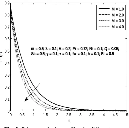
Figs. 2 – 5 present the influence of the magnetic field on the primary and secondary velocities, temperature and mass concentration. The presence of magnetic field decelerates the primary flow as a result of the resistive effect of the Lorentz force generated owing to the magnetic field which acts in the opposite direction to the fluid flow. Stronger magnetic fields result in further reduction in velocity and hence the thickness of the hydrodynamic boundary layers decreases. No secondary flow occurs in the absence of magnetic field and as the magnetic field strength increases a cross flow in the lateral direction is induced on account of the Hall currents. The secondary velocity is found to increase rapidly for increasing values of M in the vicinity of the boundary and attains its maximum and descends rapidly. For small values of M the velocity descends asymptotically to reach its free stream value. The temperature and the mass concentration are enhanced with increase in magnetic field strength and thus thermal boundary layer and mass concentration boundary layers are enlarged.
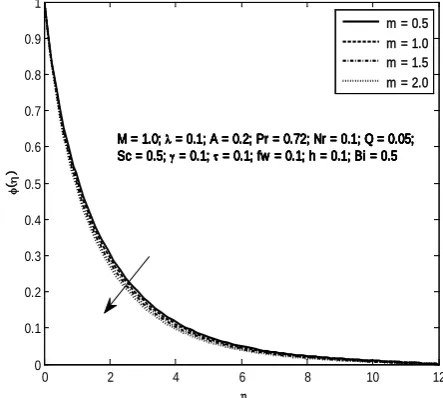
The effect of Hall parameter on the primary and secondary velocities, temperature and mass concentration is illustrated in Figs. 6 – 9. As mentioned above, the Lorentz force has a retarding effect on the primary velocity, this retardation is reduced with increase in the Hall parameter and hence the primary velocity is enhanced and consequently the hydrodynamic boundary layers become thicker. The secondary velocity increases as the Hall parameter m increases. The effect of Hall parameter on temperature and concentration is observed to be opposite to that of magnetic field. However, the variation in species concentration is small.
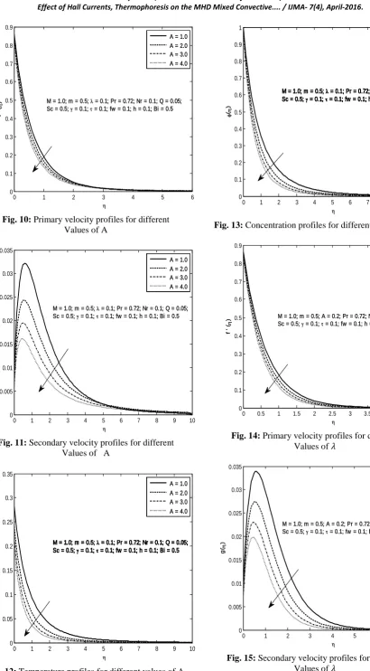
Figs. 10 – 13 reveal that primary and secondary velocities diminish with an increase in the unsteadiness parameter with a reduction in the thickness of the boundary layer. The temperature and concentration distributions also show a decreasing tendency with the unsteadiness parameter. The presence of porous medium causes a resistance to the fluid motion which leads to a reduction in both velocities (Figs. 14 and 15) and consequently the temperature and concentration rise. Fig. 16 shows that the temperature profiles increase with increasing porous parameter. Fig. 17 illustrates that the concentration increases in the solutal boundary layer with increasing values of porous parameter.
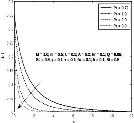
Fig. 18 presents the effect of Biot number on the thermal boundary layer. As Biot number increases convection becomes stronger resulting in higher surface temperature and the thermal effect penetrates deeper into the quiescent fluid. The thickness of corresponding thermal boundary layers increase. Fig. 19 illustrates that the temperature of higher Prandtl number fluids falls at a greater rate than the lower Prandtl number fluids. As Prandtl number is the ratio of the momentum diffusivity to thermal diffusivity, higher values of Pr correspond to diminishing of the thermal conductivity and hence the heat transfer from the heated plate takes place more rapidly for larger values of Prandtl number. Therefore, thermal boundary layer of higher Prandtl number fluids shrinks when compared to low Prandtl number fluids.
It is observed from Fig. 20 that increasing values of thermal radiation parameter produce thicker thermal boundary layers with a rise in temperature. The presence of (1 +4
3Nr)/Pr in the temperature equation (26) contributes for the
rise in temperature for higher values of thermal radiation parameter. Fig. 21 depicts that the temperature is enhanced in the presence of heat source. The heat source releases energy in the thermal boundary layer resulting in the rise of temperature. On increasing 𝑄𝑄> 0 (heat source) the temperature further rises. In the case of heat absorption 𝑄𝑄< 0 (heat sink) the temperature drops with decreasing values of 𝑄𝑄< 0 due to the absorption of energy in the thermal boundary layer.
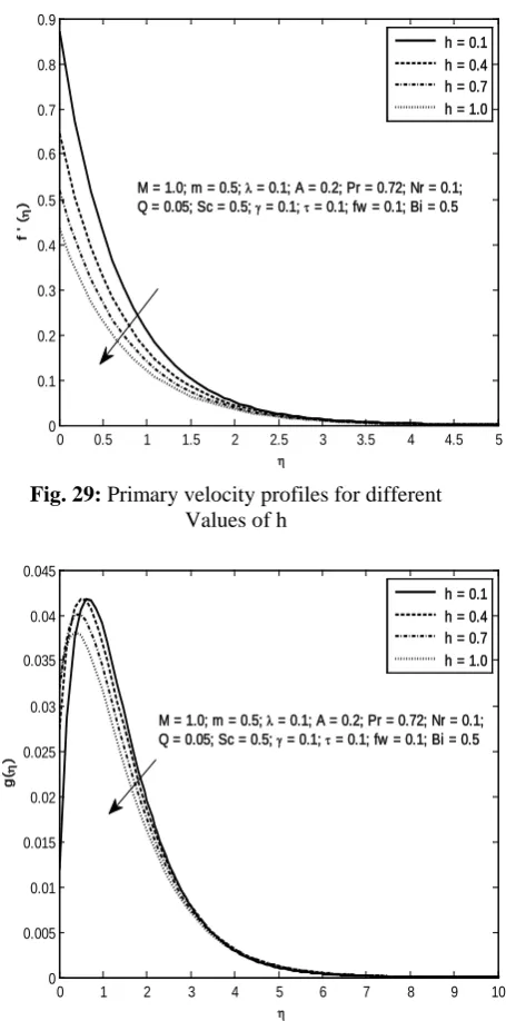
Figs. 25 – 28 depict the plots of velocities, temperature and concentration distribution for different values of suction. It is observed that the wall suction tends to reduce the thickness of the boundary layers. The temperature is observed to decrease with increasing suction parameter. Concentration is also observed to reduce for increasing values of suction. Figs. 29 and 30 display that the effect of velocity slip parameter h is to retard both the primary and secondary velocities as expected and consequently the temperature and concentration increase. It is evident from the Fig. 31 the temperature rises with increasing values of the slip parameter. The species concentration is also found to enhance for higher values of slip parameter (Fig. 32).
From Table 2 it is noted that the local skin friction coefficient CfxRex1/2 decreases for increasing values of magnetic parameter and shows an opposite trend for increasing values of Hall parameter. The skin friction coefficient CfzRez1/2 in the z-direction increases with increasing values of magnetic parameter, whereas the effect of Hall parameter is to enhance monotonically when m increases to 1.5 and reduces for values of m greater than 1.5. Salem and Aziz (2008)
also noticed the same behaviour. The heat transfer coefficient (local Nusselt number NuxRex−1/2) and the mass transfer coefficient (local Sherwood number ShxRex−1/2) are observed to decrease for increasing values of magnetic parameter (M) while a totally reversal behaviour is noticed with an increase in the Hall parameter. The skin friction coefficient in both directions decrease with increasing values of unsteady parameter and an enhancement in the Nusselt number and Sherwood number is observed. The velocity slip parameter has a decreasing influence on skin friction coefficient in x and z – directions, heat and mass transfer coefficients. It is observed that higher Prandtl number fluids have higher values of Nusselt number. The effect of thermal radiation parameter (Nr) on the Nusselt number is opposite to that of the Prandtl number. Increasing values of Nr reduces Sherwood number. Increasing values of the heat source parameter
(𝑄𝑄> 0) favour the heat and mass transfer rates whereas a reversal trend is found for increase in the sink parameter
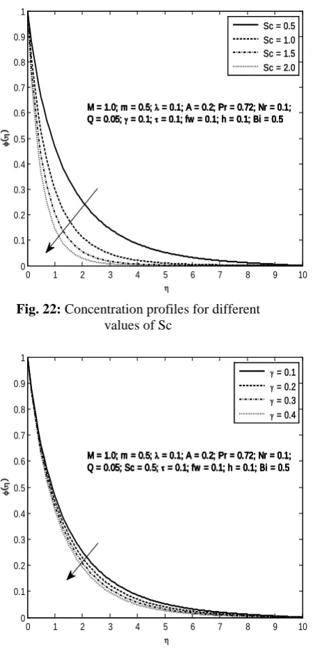
(𝑄𝑄< 0). As the Schmidt number increases, the Sherwood number enhances. The influence of chemical reaction
parameter on Sherwood number is similar to that of the Schmidt number. Increasing values of thermophoresis parameter enhances the Sherwood number. The Nusselt number and Sherwood number are observed to increase with increasing values of suction. The effect of increasing suction on the Skin friction coefficient in the both directions is to decrease whereas the local Nusselt number and the local Sherwood number are enhanced. The velocity slip parameter increases the skin friction coefficient in the x-direction while it reduces in the z-direction. The local Nusselt number and the local Sherwood number are observed to decrease for increasing values of velocity slip parameter. The Biot number has a significant effect on the heat transfer coefficient producing an enhancement for increasing values of Biot number.
Fig. 2: Primary velocity profiles for different Values of M
Fig. 3: Secondary velocity profiles for different Values of M
0 0.5 1 1.5 2 2.5 3 3.5 4 4.5 5
0 0.1 0.2 0.3 0.4 0.5 0.6 0.7 0.8 0.9
η
f '
(η
) m = 0.5; λ = 0.1; A = 0.2; Pr = 0.72; Nr = 0.1; Q = 0.05;
Sc = 0.5; γ = 0.1; τ = 0.1; fw = 0.1; h = 0.1; Bi = 0.5 m = 0.5; λ = 0.1; A = 0.2; Pr = 0.72; Nr = 0.1; Q = 0.05; Sc = 0.5; γ = 0.1; τ = 0.1; fw = 0.1; h = 0.1; Bi = 0.5 m = 0.5; λ = 0.1; A = 0.2; Pr = 0.72; Nr = 0.1; Q = 0.05; Sc = 0.5; γ = 0.1; τ = 0.1; fw = 0.1; h = 0.1; Bi = 0.5 m = 0.5; λ = 0.1; A = 0.2; Pr = 0.72; Nr = 0.1; Q = 0.05; Sc = 0.5; γ = 0.1; τ = 0.1; fw = 0.1; h = 0.1; Bi = 0.5
M = 1.0 M = 2.0 M = 3.0 M = 4.0
0 1 2 3 4 5 6 7 8
0 0.01 0.02 0.03 0.04 0.05 0.06 0.07
η
g(
η
)
m = 0.5; λ = 0.1; A = 0.2; Pr = 0.72; Nr = 0.1; Q = 0.05; Sc = 0.5; γ = 0.1; τ = 0.1; fw = 0.1; h = 0.1; Bi = 0.5 m = 0.5; λ = 0.1; A = 0.2; Pr = 0.72; Nr = 0.1; Q = 0.05; Sc = 0.5; γ = 0.1; τ = 0.1; fw = 0.1; h = 0.1; Bi = 0.5 m = 0.5; λ = 0.1; A = 0.2; Pr = 0.72; Nr = 0.1; Q = 0.05; Sc = 0.5; γ = 0.1; τ = 0.1; fw = 0.1; h = 0.1; Bi = 0.5 m = 0.5; λ = 0.1; A = 0.2; Pr = 0.72; Nr = 0.1; Q = 0.05; Sc = 0.5; γ = 0.1; τ = 0.1; fw = 0.1; h = 0.1; Bi = 0.5
Fig. 4: Temperature profiles for different values of M
Fig. 5: Concentration profiles for different values of M
Fig. 6: Primary velocity profiles for different Values of m
Fig. 7: Secondary velocity profiles for different Values of m
Fig. 8: Temperature profiles for different values of m
Fig. 9: Concentration profiles for different values of m
0 2 4 6 8 10 12
0 0.05 0.1 0.15 0.2 0.25 0.3 0.35 0.4
η
θ
(η
)
m = 0.5; λ = 0.1; A = 0.2; Pr = 0.72; Nr = 0.1; Q = 0.05; Sc = 0.5; γ = 0.1; τ = 0.1; fw = 0.1; h = 0.1; Bi = 0.5 m = 0.5; λ = 0.1; A = 0.2; Pr = 0.72; Nr = 0.1; Q = 0.05; Sc = 0.5; γ = 0.1; τ = 0.1; fw = 0.1; h = 0.1; Bi = 0.5 m = 0.5; λ = 0.1; A = 0.2; Pr = 0.72; Nr = 0.1; Q = 0.05; Sc = 0.5; γ = 0.1; τ = 0.1; fw = 0.1; h = 0.1; Bi = 0.5 m = 0.5; λ = 0.1; A = 0.2; Pr = 0.72; Nr = 0.1; Q = 0.05; Sc = 0.5; γ = 0.1; τ = 0.1; fw = 0.1; h = 0.1; Bi = 0.5
M = 1.0 M = 2.0 M = 3.0 M = 4.0
0 2 4 6 8 10 12
0 0.1 0.2 0.3 0.4 0.5 0.6 0.7 0.8 0.9 1
η
φ
(η
)
m = 0.5; λ = 0.1; A = 0.2; Pr = 0.72; Nr = 0.1; Q = 0.05; Sc = 0.5; γ = 0.1; τ = 0.1; fw = 0.1; h = 0.1; Bi = 0.5 m = 0.5; λ = 0.1; A = 0.2; Pr = 0.72; Nr = 0.1; Q = 0.05; Sc = 0.5; γ = 0.1; τ = 0.1; fw = 0.1; h = 0.1; Bi = 0.5 m = 0.5; λ = 0.1; A = 0.2; Pr = 0.72; Nr = 0.1; Q = 0.05; Sc = 0.5; γ = 0.1; τ = 0.1; fw = 0.1; h = 0.1; Bi = 0.5 m = 0.5; λ = 0.1; A = 0.2; Pr = 0.72; Nr = 0.1; Q = 0.05; Sc = 0.5; γ = 0.1; τ = 0.1; fw = 0.1; h = 0.1; Bi = 0.5
M = 1.0 M = 2.0 M = 3.0 M = 4.0
0 0.5 1 1.5 2 2.5 3 3.5 4 4.5 5
0 0.1 0.2 0.3 0.4 0.5 0.6 0.7 0.8 0.9
η
f '
(η
) M = 1.0; λ = 0.1; A = 0.2; Pr = 0.72; Nr = 0.1; Q = 0.05;
Sc = 0.5; γ = 0.1; τ = 0.1; fw = 0.1; h = 0.1; Bi = 0.5 m = 0.5 m = 1.0 m = 1.5 m = 2.0
0 1 2 3 4 5 6 7 8
0 0.02 0.04 0.06 0.08 0.1 0.12 0.14
η
g(
η
)
M = 1.0; λ = 0.1; A = 0.2; Pr = 0.72; Nr = 0.1; Q = 0.05; Sc = 0.5; γ = 0.1; τ = 0.1; fw = 0.1; h = 0.1; Bi = 0.5
m = 0.5 m = 1.0 m = 1.5 m = 2.0
0 2 4 6 8 10 12
0 0.05 0.1 0.15 0.2 0.25 0.3 0.35 0.4
η
θ
(η
) M = 1.0; λ = 0.1; A = 0.2; Pr = 0.72; Nr = 0.1; Q = 0.05;
Sc = 0.5; γ = 0.1; τ = 0.1; fw = 0.1; h = 0.1; Bi = 0.5 M = 1.0; λ = 0.1; A = 0.2; Pr = 0.72; Nr = 0.1; Q = 0.05; Sc = 0.5; γ = 0.1; τ = 0.1; fw = 0.1; h = 0.1; Bi = 0.5 M = 1.0; λ = 0.1; A = 0.2; Pr = 0.72; Nr = 0.1; Q = 0.05; Sc = 0.5; γ = 0.1; τ = 0.1; fw = 0.1; h = 0.1; Bi = 0.5 M = 1.0; λ = 0.1; A = 0.2; Pr = 0.72; Nr = 0.1; Q = 0.05; Sc = 0.5; γ = 0.1; τ = 0.1; fw = 0.1; h = 0.1; Bi = 0.5
m = 0.5 m = 1.0 m = 1.5 m = 2.0
0 2 4 6 8 10 12
0 0.1 0.2 0.3 0.4 0.5 0.6 0.7 0.8 0.9 1
η
φ
(η
)
M = 1.0; λ = 0.1; A = 0.2; Pr = 0.72; Nr = 0.1; Q = 0.05; Sc = 0.5; γ = 0.1; τ = 0.1; fw = 0.1; h = 0.1; Bi = 0.5 M = 1.0; λ = 0.1; A = 0.2; Pr = 0.72; Nr = 0.1; Q = 0.05; Sc = 0.5; γ = 0.1; τ = 0.1; fw = 0.1; h = 0.1; Bi = 0.5 M = 1.0; λ = 0.1; A = 0.2; Pr = 0.72; Nr = 0.1; Q = 0.05; Sc = 0.5; γ = 0.1; τ = 0.1; fw = 0.1; h = 0.1; Bi = 0.5 M = 1.0; λ = 0.1; A = 0.2; Pr = 0.72; Nr = 0.1; Q = 0.05; Sc = 0.5; γ = 0.1; τ = 0.1; fw = 0.1; h = 0.1; Bi = 0.5
Fig. 10: Primary velocity profiles for different Values of A
Fig. 11: Secondary velocity profiles for different Values of A
Fig. 12: Temperature profiles for different values of A
Fig. 13: Concentration profiles for different values of A
Fig. 14: Primary velocity profiles for different Values of 𝜆𝜆
Fig. 15: Secondary velocity profiles for different Values of 𝜆𝜆
0 1 2 3 4 5 6
0 0.1 0.2 0.3 0.4 0.5 0.6 0.7 0.8 0.9
η
f '
(η
) M = 1.0; m = 0.5; λ = 0.1; Pr = 0.72; Nr = 0.1; Q = 0.05; Sc = 0.5; γ = 0.1; τ = 0.1; fw = 0.1; h = 0.1; Bi = 0.5
A = 1.0 A = 2.0 A = 3.0 A = 4.0
0 1 2 3 4 5 6 7 8 9 10
0 0.005 0.01 0.015 0.02 0.025 0.03 0.035
η
g(
η
)
M = 1.0; m = 0.5; λ = 0.1; Pr = 0.72; Nr = 0.1; Q = 0.05; Sc = 0.5; γ = 0.1; τ = 0.1; fw = 0.1; h = 0.1; Bi = 0.5
A = 1.0 A = 2.0 A = 3.0 A = 4.0
0 1 2 3 4 5 6 7 8 9 10
0 0.05 0.1 0.15 0.2 0.25 0.3 0.35
η
θ
(η
)
M = 1.0; m = 0.5; λ = 0.1; Pr = 0.72; Nr = 0.1; Q = 0.05; Sc = 0.5; γ = 0.1; τ = 0.1; fw = 0.1; h = 0.1; Bi = 0.5 M = 1.0; m = 0.5; λ = 0.1; Pr = 0.72; Nr = 0.1; Q = 0.05; Sc = 0.5; γ = 0.1; τ = 0.1; fw = 0.1; h = 0.1; Bi = 0.5 M = 1.0; m = 0.5; λ = 0.1; Pr = 0.72; Nr = 0.1; Q = 0.05; Sc = 0.5; γ = 0.1; τ = 0.1; fw = 0.1; h = 0.1; Bi = 0.5 M = 1.0; m = 0.5; λ = 0.1; Pr = 0.72; Nr = 0.1; Q = 0.05; Sc = 0.5; γ = 0.1; τ = 0.1; fw = 0.1; h = 0.1; Bi = 0.5
A = 1.0 A = 2.0 A = 3.0 A = 4.0
0 1 2 3 4 5 6 7 8 9 10
0 0.1 0.2 0.3 0.4 0.5 0.6 0.7 0.8 0.9 1
η
φ
(η
)
M = 1.0; m = 0.5; λ = 0.1; Pr = 0.72; Nr = 0.1; Q = 0.05; Sc = 0.5; γ = 0.1; τ = 0.1; fw = 0.1; h = 0.1; Bi = 0.5 M = 1.0; m = 0.5; λ = 0.1; Pr = 0.72; Nr = 0.1; Q = 0.05; Sc = 0.5; γ = 0.1; τ = 0.1; fw = 0.1; h = 0.1; Bi = 0.5 M = 1.0; m = 0.5; λ = 0.1; Pr = 0.72; Nr = 0.1; Q = 0.05; Sc = 0.5; γ = 0.1; τ = 0.1; fw = 0.1; h = 0.1; Bi = 0.5 M = 1.0; m = 0.5; λ = 0.1; Pr = 0.72; Nr = 0.1; Q = 0.05; Sc = 0.5; γ = 0.1; τ = 0.1; fw = 0.1; h = 0.1; Bi = 0.5
A = 1.0 A = 2.0 A = 3.0 A = 4.0
0 0.5 1 1.5 2 2.5 3 3.5 4 4.5 5
0 0.1 0.2 0.3 0.4 0.5 0.6 0.7 0.8 0.9
η
f '
(η
) M = 1.0; m = 0.5; A = 0.2; Pr = 0.72; Nr = 0.1; Q = 0.05;
Sc = 0.5; γ = 0.1; τ = 0.1; fw = 0.1; h = 0.1; Bi = 0.5
λ = 0.5
λ = 1.0
λ = 1.5
λ = 2.0
0 1 2 3 4 5 6 7 8
0 0.005 0.01 0.015 0.02 0.025 0.03 0.035
η
g(
η
)
M = 1.0; m = 0.5; A = 0.2; Pr = 0.72; Nr = 0.1; Q = 0.05; Sc = 0.5; γ = 0.1; τ = 0.1; fw = 0.1; h = 0.1; Bi = 0.5
λ = 0.5
λ = 1.0
λ = 1.5
Fig. 16: Temperature profiles for different values of 𝜆𝜆
Fig. 17: Concentration profiles for different values of 𝜆𝜆
Fig. 18: Temperature profiles for different values of Bi
Fig. 19: Temperature profiles for different values of Pr
Fig. 20: Temperature profiles for different values of Nr
Fig. 21: Temperature profiles for different values of Q
0 2 4 6 8 10 12
0 0.05 0.1 0.15 0.2 0.25 0.3 0.35 0.4
η
θ
(η
) M = 1.0; m = 0.5; A = 0.2; Pr = 0.72; Nr = 0.1; Q = 0.05;
Sc = 0.5; γ = 0.1; τ = 0.1; fw = 0.1; h = 0.1; Bi = 0.5 M = 1.0; m = 0.5; A = 0.2; Pr = 0.72; Nr = 0.1; Q = 0.05; Sc = 0.5; γ = 0.1; τ = 0.1; fw = 0.1; h = 0.1; Bi = 0.5 M = 1.0; m = 0.5; A = 0.2; Pr = 0.72; Nr = 0.1; Q = 0.05; Sc = 0.5; γ = 0.1; τ = 0.1; fw = 0.1; h = 0.1; Bi = 0.5 M = 1.0; m = 0.5; A = 0.2; Pr = 0.72; Nr = 0.1; Q = 0.05; Sc = 0.5; γ = 0.1; τ = 0.1; fw = 0.1; h = 0.1; Bi = 0.5
λ = 0.5
λ = 1.0
λ = 1.5
λ = 2.0
0 2 4 6 8 10 12
0 0.1 0.2 0.3 0.4 0.5 0.6 0.7 0.8 0.9 1
η
φ
(η
)
M = 1.0; m = 0.5; A = 0.2; Pr = 0.72; Nr = 0.1; Q = 0.05; Sc = 0.5; γ = 0.1; τ = 0.1; fw = 0.1; h = 0.1; Bi = 0.5 M = 1.0; m = 0.5; A = 0.2; Pr = 0.72; Nr = 0.1; Q = 0.05; Sc = 0.5; γ = 0.1; τ = 0.1; fw = 0.1; h = 0.1; Bi = 0.5 M = 1.0; m = 0.5; A = 0.2; Pr = 0.72; Nr = 0.1; Q = 0.05; Sc = 0.5; γ = 0.1; τ = 0.1; fw = 0.1; h = 0.1; Bi = 0.5 M = 1.0; m = 0.5; A = 0.2; Pr = 0.72; Nr = 0.1; Q = 0.05; Sc = 0.5; γ = 0.1; τ = 0.1; fw = 0.1; h = 0.1; Bi = 0.5
λ = 0.5
λ = 1.0
λ = 1.5
λ = 2.0
0 2 4 6 8 10 12
0 0.1 0.2 0.3 0.4 0.5
η
θ
(η
) M = 1.0; m = 0.5; λ = 0.1; A = 0.2; Pr = 0.72; Nr = 0.1;
Q = 0.05; Sc = 0.5; γ = 0.1; τ = 0.1; fw = 0.1; h = 0.1 M = 1.0; m = 0.5; λ = 0.1; A = 0.2; Pr = 0.72; Nr = 0.1; Q = 0.05; Sc = 0.5; γ = 0.1; τ = 0.1; fw = 0.1; h = 0.1 M = 1.0; m = 0.5; λ = 0.1; A = 0.2; Pr = 0.72; Nr = 0.1; Q = 0.05; Sc = 0.5; γ = 0.1; τ = 0.1; fw = 0.1; h = 0.1 M = 1.0; m = 0.5; λ = 0.1; A = 0.2; Pr = 0.72; Nr = 0.1; Q = 0.05; Sc = 0.5; γ = 0.1; τ = 0.1; fw = 0.1; h = 0.1
Bi = 0.1 Bi = 0.4 Bi = 0.7 Bi = 1.0
0 2 4 6 8 10 12
0 0.05 0.1 0.15 0.2 0.25 0.3 0.35 0.4
η
θ
(η
) M = 1.0; m = 0.5; λ = 0.1; A = 0.2; Nr = 0.1; Q = 0.05;
Sc = 0.5; γ = 0.1; τ = 0.1; fw = 0.1; h = 0.1; Bi = 0.5 M = 1.0; m = 0.5; λ = 0.1; A = 0.2; Nr = 0.1; Q = 0.05; Sc = 0.5; γ = 0.1; τ = 0.1; fw = 0.1; h = 0.1; Bi = 0.5 M = 1.0; m = 0.5; λ = 0.1; A = 0.2; Nr = 0.1; Q = 0.05; Sc = 0.5; γ = 0.1; τ = 0.1; fw = 0.1; h = 0.1; Bi = 0.5 M = 1.0; m = 0.5; λ = 0.1; A = 0.2; Nr = 0.1; Q = 0.05; Sc = 0.5; γ = 0.1; τ = 0.1; fw = 0.1; h = 0.1; Bi = 0.5
Pr = 0.72 Pr = 1.0 Pr = 2.0 Pr = 3.0
0 2 4 6 8 10 12
0 0.05 0.1 0.15 0.2 0.25 0.3 0.35 0.4 0.45 0.5
η
θ
(η
)
M = 1.0; m = 0.5; λ = 0.1; A = 0.2; Pr = 0.72; Q = 0.05; Sc = 0.5; γ = 0.1; τ = 0.1; fw = 0.1; h = 0.1; Bi = 0.5 M = 1.0; m = 0.5; λ = 0.1; A = 0.2; Pr = 0.72; Q = 0.05; Sc = 0.5; γ = 0.1; τ = 0.1; fw = 0.1; h = 0.1; Bi = 0.5 M = 1.0; m = 0.5; λ = 0.1; A = 0.2; Pr = 0.72; Q = 0.05; Sc = 0.5; γ = 0.1; τ = 0.1; fw = 0.1; h = 0.1; Bi = 0.5 M = 1.0; m = 0.5; λ = 0.1; A = 0.2; Pr = 0.72; Q = 0.05; Sc = 0.5; γ = 0.1; τ = 0.1; fw = 0.1; h = 0.1; Bi = 0.5
Nr = 0.1 Nr = 0.4 Nr = 0.7 Nr = 1.0
0 2 4 6 8 10 12
0 0.05 0.1 0.15 0.2 0.25 0.3 0.35 0.4
η
θ
(η
) M = 1.0; m = 0.5; λ = 0.1; A = 0.2; Pr = 0.72; Nr = 0.1;
Sc = 0.5; γ = 0.1; τ = 0.1; fw = 0.1; h = 0.1; Bi = 0.5 M = 1.0; m = 0.5; λ = 0.1; A = 0.2; Pr = 0.72; Nr = 0.1; Sc = 0.5; γ = 0.1; τ = 0.1; fw = 0.1; h = 0.1; Bi = 0.5 M = 1.0; m = 0.5; λ = 0.1; A = 0.2; Pr = 0.72; Nr = 0.1; Sc = 0.5; γ = 0.1; τ = 0.1; fw = 0.1; h = 0.1; Bi = 0.5 M = 1.0; m = 0.5; λ = 0.1; A = 0.2; Pr = 0.72; Nr = 0.1; Sc = 0.5; γ = 0.1; τ = 0.1; fw = 0.1; h = 0.1; Bi = 0.5 M = 1.0; m = 0.5; λ = 0.1; A = 0.2; Pr = 0.72; Nr = 0.1; Sc = 0.5; γ = 0.1; τ = 0.1; fw = 0.1; h = 0.1; Bi = 0.5
Fig. 22: Concentration profiles for different values of Sc
Fig. 23: Concentration profiles for different values of 𝛾𝛾
Fig. 24: Concentration profiles for different values of 𝜏𝜏
Fig. 25: Primary velocity profiles for different Values of fw
Fig. 26: Secondary velocity profiles for different Values of fw
Fig. 27: Temperature profiles for different values of fw
0 1 2 3 4 5 6 7 8 9 10
0 0.1 0.2 0.3 0.4 0.5 0.6 0.7 0.8 0.9 1
η
φ
(η
)
M = 1.0; m = 0.5; λ = 0.1; A = 0.2; Pr = 0.72; Nr = 0.1; Q = 0.05; γ = 0.1; τ = 0.1; fw = 0.1; h = 0.1; Bi = 0.5 M = 1.0; m = 0.5; λ = 0.1; A = 0.2; Pr = 0.72; Nr = 0.1; Q = 0.05; γ = 0.1; τ = 0.1; fw = 0.1; h = 0.1; Bi = 0.5 M = 1.0; m = 0.5; λ = 0.1; A = 0.2; Pr = 0.72; Nr = 0.1; Q = 0.05; γ = 0.1; τ = 0.1; fw = 0.1; h = 0.1; Bi = 0.5 M = 1.0; m = 0.5; λ = 0.1; A = 0.2; Pr = 0.72; Nr = 0.1; Q = 0.05; γ = 0.1; τ = 0.1; fw = 0.1; h = 0.1; Bi = 0.5
Sc = 0.5 Sc = 1.0 Sc = 1.5 Sc = 2.0
0 1 2 3 4 5 6 7 8 9 10
0 0.1 0.2 0.3 0.4 0.5 0.6 0.7 0.8 0.9 1
η
φ
(η
)
M = 1.0; m = 0.5; λ = 0.1; A = 0.2; Pr = 0.72; Nr = 0.1; Q = 0.05; Sc = 0.5; τ = 0.1; fw = 0.1; h = 0.1; Bi = 0.5 M = 1.0; m = 0.5; λ = 0.1; A = 0.2; Pr = 0.72; Nr = 0.1; Q = 0.05; Sc = 0.5; τ = 0.1; fw = 0.1; h = 0.1; Bi = 0.5 M = 1.0; m = 0.5; λ = 0.1; A = 0.2; Pr = 0.72; Nr = 0.1; Q = 0.05; Sc = 0.5; τ = 0.1; fw = 0.1; h = 0.1; Bi = 0.5 M = 1.0; m = 0.5; λ = 0.1; A = 0.2; Pr = 0.72; Nr = 0.1; Q = 0.05; Sc = 0.5; τ = 0.1; fw = 0.1; h = 0.1; Bi = 0.5
γ = 0.1
γ = 0.2
γ = 0.3
γ = 0.4
0 1 2 3 4 5 6 7 8 9 10
0 0.1 0.2 0.3 0.4 0.5 0.6 0.7 0.8 0.9 1
η
φ
(η
) M = 1.0; m = 0.5; λ = 0.1; A = 0.2; Pr = 0.72; Nr = 0.1;
Q = 0.05; Sc = 0.5; γ = 0.1; fw = 0.1; h = 0.1; Bi = 0.5 M = 1.0; m = 0.5; λ = 0.1; A = 0.2; Pr = 0.72; Nr = 0.1; Q = 0.05; Sc = 0.5; γ = 0.1; fw = 0.1; h = 0.1; Bi = 0.5 M = 1.0; m = 0.5; λ = 0.1; A = 0.2; Pr = 0.72; Nr = 0.1; Q = 0.05; Sc = 0.5; γ = 0.1; fw = 0.1; h = 0.1; Bi = 0.5 M = 1.0; m = 0.5; λ = 0.1; A = 0.2; Pr = 0.72; Nr = 0.1; Q = 0.05; Sc = 0.5; γ = 0.1; fw = 0.1; h = 0.1; Bi = 0.5
τ = 1.0
τ = 2.0
τ = 3.0
τ = 4.0
0 0.5 1 1.5 2 2.5 3 3.5 4 4.5 5
0 0.1 0.2 0.3 0.4 0.5 0.6 0.7 0.8 0.9
η
f '
(η
)
M = 1.0; m = 0.5; λ = 0.1; A = 0.2; Pr = 0.72; Nr = 0.1; Q = 0.05; Sc = 0.5; γ = 0.1; τ = 0.1; h = 0.1; Bi = 0.5
fw = 0.1 fw = 0.4 fw = 0.7 fw = 1.0
0 1 2 3 4 5 6 7 8 9 10
0 0.005 0.01 0.015 0.02 0.025 0.03 0.035 0.04 0.045
η
g(
η
)
M = 1.0; m = 0.5; λ = 0.1; A = 0.2; Pr = 0.72; Nr = 0.1; Q = 0.05; Sc = 0.5; γ = 0.1; τ = 0.1; h = 0.1; Bi = 0.5
fw = 0.1 fw = 0.4 fw = 0.7 fw = 1.0
0 2 4 6 8 10 12
0 0.05 0.1 0.15 0.2 0.25 0.3 0.35
η
θ
(η
)
M = 1.0; m = 0.5; λ = 0.1; A = 0.2; Pr = 0.72; Nr = 0.1; Q = 0.05; Sc = 0.5; γ = 0.1; τ = 0.1; h = 0.1; Bi = 0.5 M = 1.0; m = 0.5; λ = 0.1; A = 0.2; Pr = 0.72; Nr = 0.1; Q = 0.05; Sc = 0.5; γ = 0.1; τ = 0.1; h = 0.1; Bi = 0.5 M = 1.0; m = 0.5; λ = 0.1; A = 0.2; Pr = 0.72; Nr = 0.1; Q = 0.05; Sc = 0.5; γ = 0.1; τ = 0.1; h = 0.1; Bi = 0.5 M = 1.0; m = 0.5; λ = 0.1; A = 0.2; Pr = 0.72; Nr = 0.1; Q = 0.05; Sc = 0.5; γ = 0.1; τ = 0.1; h = 0.1; Bi = 0.5
Fig. 28: Concentration profiles for different values of w
Fig. 29: Primary velocity profiles for different Values of h
Fig. 30: Secondary velocity profiles for different Values of h
Fig. 31: Temperature profiles for different values of h
Fig. 32: Concentration profiles for different values of h
0 2 4 6 8 10 12
0 0.1 0.2 0.3 0.4 0.5 0.6 0.7 0.8 0.9 1
η
φ
(η
)
M = 1.0; m = 0.5; λ = 0.1; A = 0.2; Pr = 0.72; Nr = 0.1; Q = 0.05; Sc = 0.5; γ = 0.1; τ = 0.1; h = 0.1; Bi = 0.5 M = 1.0; m = 0.5; λ = 0.1; A = 0.2; Pr = 0.72; Nr = 0.1; Q = 0.05; Sc = 0.5; γ = 0.1; τ = 0.1; h = 0.1; Bi = 0.5 M = 1.0; m = 0.5; λ = 0.1; A = 0.2; Pr = 0.72; Nr = 0.1; Q = 0.05; Sc = 0.5; γ = 0.1; τ = 0.1; h = 0.1; Bi = 0.5 M = 1.0; m = 0.5; λ = 0.1; A = 0.2; Pr = 0.72; Nr = 0.1; Q = 0.05; Sc = 0.5; γ = 0.1; τ = 0.1; h = 0.1; Bi = 0.5
fw = 0.1 fw = 0.4 fw = 0.7 fw = 1.0
0 0.5 1 1.5 2 2.5 3 3.5 4 4.5 5
0 0.1 0.2 0.3 0.4 0.5 0.6 0.7 0.8 0.9
η
f '
(η
)
M = 1.0; m = 0.5; λ = 0.1; A = 0.2; Pr = 0.72; Nr = 0.1; Q = 0.05; Sc = 0.5; γ = 0.1; τ = 0.1; fw = 0.1; Bi = 0.5
h = 0.1 h = 0.4 h = 0.7 h = 1.0
0 1 2 3 4 5 6 7 8 9 10
0 0.005 0.01 0.015 0.02 0.025 0.03 0.035 0.04 0.045
η
g(
η
)
M = 1.0; m = 0.5; λ = 0.1; A = 0.2; Pr = 0.72; Nr = 0.1; Q = 0.05; Sc = 0.5; γ = 0.1; τ = 0.1; fw = 0.1; Bi = 0.5 h = 0.1 h = 0.4 h = 0.7 h = 1.0
0 2 4 6 8 10 12
0 0.05 0.1 0.15 0.2 0.25 0.3 0.35 0.4 0.45
η
θ
(η
)
M = 1.0; m = 0.5; λ = 0.1; A = 0.2; Pr = 0.72; Nr = 0.1; Q = 0.05; Sc = 0.5; γ = 0.1; τ = 0.1; fw = 0.1; Bi = 0.5
h = 0.1
h = 0.4 h = 0.7 h = 1.0
0 2 4 6 8 10 12
0 0.1 0.2 0.3 0.4 0.5 0.6 0.7 0.8 0.9 1
η
φ
(η
)
M = 1.0; m = 0.5; λ = 0.1; A = 0.2; Pr = 0.72; Nr = 0.1; Q = 0.05; Sc = 0.5; γ = 0.1; τ = 0.1; fw = 0.1; Bi = 0.5 M = 1.0; m = 0.5; λ = 0.1; A = 0.2; Pr = 0.72; Nr = 0.1; Q = 0.05; Sc = 0.5; γ = 0.1; τ = 0.1; fw = 0.1; Bi = 0.5 M = 1.0; m = 0.5; λ = 0.1; A = 0.2; Pr = 0.72; Nr = 0.1; Q = 0.05; Sc = 0.5; γ = 0.1; τ = 0.1; fw = 0.1; Bi = 0.5 M = 1.0; m = 0.5; λ = 0.1; A = 0.2; Pr = 0.72; Nr = 0.1; Q = 0.05; Sc = 0.5; γ = 0.1; τ = 0.1; fw = 0.1; Bi = 0.5
Table-2: Skin friction, Nusselt number and Sherwood number values for variation of different parameters
M m 𝝀𝝀 A Pr Nr Q Sc 𝜸𝜸 𝝉𝝉 fw h Bi 𝒇𝒇′′(𝟎𝟎) 𝒈𝒈′(𝟎𝟎) −𝜽𝜽′(𝟎𝟎) −𝝓𝝓′(𝟎𝟎)
1.0 2.0 3.0 4.0
0.5 0.1 0.2 0.72 0.1 0.05 0.5 0.1 0.1 0.1 0.1 0.5
-1.264241 -1.467105 -1.635682 -1.781029 0.119336 0.185284 0.230889 0.265597 0.327964 0.320399 0.314233 0.309072 0.891038 0.842532 0.806391 0.778115 1.0 0.5 1.0 1.5 2.0
0.1 0.2 0.72 0.1 0.05 0.5 0.1 0.1 0.1 0.1 0.5
-1.635682 -1.489627 -1.366128 -1.277822 0.230889 0.341715 0.366866 0.356532 0.314054 0.318066 0.322012 0.325199 0.805726 0.829097 0.853121 0.873365
1.0 0.5 0.5 1.0 1.5 2.0
0.2 0.72 0.1 0.05 0.5 0.1 0.1 0.1 0.1 0.5
-1.363510 -1.474763 -1.574795 -1.665912 0.104729 0.091541 0.081764 0.074161 0.320803 0.316467 0.312585 0.309082 0.867348 0.842722 0.821762 0.803643
1.0 0.5 0.1 1.0 2.0 3.0 4.0
0.72 0.1 0.05 0.5 0.1 0.1 0.1 0.1 0.5
-1.408287 -1.566642 -1.705245 -1.828476 0.099135 0.082021 0.070403 0.061982 0.358930 0.379277 0.392007 0.401107 1.173619 1.431517 1.644543 1.831261
1.0 0.5 0.1 0.2 0.72
1.0 2.0 3.0
0.1 0.05 0.5 0.1 0.1 0.1 0.1 0.5
-1.264241 -1.264241 -1.264241 -1.264241 0.119336 0.119336 0.119336 0.119336 0.324653 0.348666 0.391116 0.410906 0.890432 0.891592 0.893871 0.895081
1.0 0.5 0.1 0.2 0.72 0.0 0.4 0.7 1.0
0.05 0.5 0.1 0.1 0.1 0.1 0.5
-1.264241 -1.264241 -1.264241 -1.264241 0.119336 0.119336 0.119336 0.119336 0.324653 0.300630 0.281249 0.265140 0.890432 0.889333 0.888482 0.887792
1.0 0.5 0.1 0.2 0.72 0.1 -0.2 -0.1 0.0 0.1 0.2
0.5 0.1 0.1 0.1 0.1 0.5
-1.262779 -1.262779 -1.262779 -1.262779 -1.262779 0.136572 0.136572 0.136572 0.136572 0.136572 0.340123 0.335802 0.330788 0.324712 0.316635 0.891431 0.891242 0.891031 0.890791 0.890500
1.0 0.5 0.1 0.2 0.72 0.1 0.05 0.5 1.0 1.5 2.0
0.1 0.1 0.1 0.1 0.5
-1.264241 -1.264241 -1.264241 -1.264241 0.119336 0.119336 0.119336 0.119336 0.327884 0.327884 0.327884 0.327884 0.890631 1.380384 1.773092 2.112501
1.0 0.5 0.1 0.2 0.72 0.1 0.05 0.5 0.1 0.2 0.3 0.4
0.1 0.1 0.1 0.5
-1.264241 -1.264241 -1.264241 -1.264241 0.119336 0.119336 0.119336 0.119336 0.327884 0.327884 0.327884 0.327884 0.890631 0.928797 0.964089 0.997157
1.0 0.5 0.1 0.2 0.72 0.1 0.05 0.5 0.1 1.0 2.0 3.0 4.0
0.1 0.1 0.5
-1.264241 -1.264241 -1.264241 -1.264241 0.119336 0.119336 0.119336 0.119336 0.327884 0.327884 0.327884 0.327884 1.003359 1.130770 1.260335 1.391933
1.0 0.5 0.1 0.2 0.72 0.1 0.05 0.5 0.1 0.1 0.1 0.4 0.7 1.0
0.1 0.5
-1.264241 -1.382407 -1.508543 -1.641429 0.119336 0.115093 0.109384 0.102609 0.327865 0.337325 0.347019 0.356653 0.890557 0.953862 1.025550 1.105822
1.0 0.5 0.1 0.2 0.72 0.1 0.05 0.5 0.1 0.1 0.1 0.1 0.4 0.7 1.0 0.5 -1.264241 -0.884522 -0.687008 -0.563935 0.119336 0.068468 0.045507 0.032785 0.327865 0.312253 0.301282 0.292919 0.890557 0.794219 0.736063 0.696102
1.0 0.5 0.1 0.2 0.72 0.1 0.05 0.5 0.1 0.1 0.1 0.1 0.1 0.4 0.7 1.0 -1.264241 -1.264241 -1.264241 -1.264241 0.119336 0.119336 0.119336 0.119336 0.090497 0.281688 0.403453 0.487796 0.881571 0.888808 0.893421 0.896618 4. CONCLUSIONS
The following conclusions are drawn:
The Lorentz force has a retarding effect on the primary velocity and an opposite effect on the secondary velocity. Temperature enhances with higher values of porous parameter, Biot number, velocity slip parameter, heat source
parameter, thermal radiation parameter and magnetic parameter while a reverse trend is observed with increase in the Hall parameter, unsteady parameter, suction parameter, heat sink parameter and Prandtl number.
The skin friction coefficient in the x-direction increases with decrease in the magnetic parameter, unsteady and porous parameters and suction. The rate of heat transfer and mass transfer increase with increasing values of magnetic parameter and velocity slip parameter while a reverse effect is observed for increasing values of Hall parameter.
The heat generation, thermal radiation favour rate of heat transfer.
The thermophoretic parameter, Schmidt number, unsteady parameter and chemical reaction parameter have an enhancing influence on Sherwood number.
5. REFERENCES
1. Aziz M. A. E., Flow and heat transfer over an unsteady stretching surface with Hall effect, Meccanica, 45 (2010), 97 – 109.
2. Chen, C. H. Laminar mixed convection adjacent to vertical continuously stretching sheets, Heat and Mass Transfer, 33 (1998), 471 – 476.
3. Dulal Pal., Hall current and MHD effects on heat transfer over an unsteady stretching permeable surface with thermal radiation”, Computers and Mathematics with Applications, 66 (2013), 1161 – 1180.
4. Eldahab E. M. A., Aziz M. A. E., Salem A. M., Jaber K. K., Hall current on MHD mixed convection flow from an inclined continuously stretching surface with blowing/suction and internal heat generation/absorption, Applied Mathematical Modelling, 31 (2007), 1829 – 1846
5. Goldsmith P. and May F.G., Diffusiophoresis and thermophoresis in water vapour systems, in Aerosol Science, Davies C.N. Davies (Ed.), Aerosol Science, Academic Press, London, (1966), 163 – 194.
6. Grubka L. J., Bobba K. M., Heat transfer characteristics of a continuous stretching surface with variable temperature, ASME J. Heat Transfer, 107 (1985), 248
7. Hales. J. M., Schwendiman L. C., Horst T. W., Aerosol transport in a naturally-convected boundary layer, Int. J. Heat Mass Transfer, 15 (1972), 1837 – 1849.
8. Sakiadis B. C., Boundary layer behavior on continuous solid surfaces: Ι. Boundary layer equations for two dimensional and axis symmetric flow, AΙChE J., 7(26) (1961).
9. Salem A. M., Abd El – Aziz M., Effect of Hall currents and chemical reaction on hydromagnetic flow of a stretching vertical surface with internal heat generation/absorption, Applied Mathematical Modelling, 32 (2008), 1236 – 1254.
10. Seddeek M. A., Effects of radiation and variable viscosity on a MHD free convection flow past a semi-infinite flat plate with an aligned magnetic field in the case of unsteady flow, Int. J. Heat Mass Transfer, 45 (2002), 931 – 5.
11. Selim A., Hossain M. A., Rees D. A. S., The effect of surface mass transfer on mixed convection flow past a heated vertical flat plate permeable plate with thermophoresis, Int. J. of Thermal Sciences, 42 (2003), 973 – 982.
12. Talbot L., Cheng R. K., Schefer A. W., Wills D. R., Thermophoresis of particles in a heated boundary layer”, Journal of Fluid Mechanics, 101(4) (1980), 737-758.
13. Vajravelu K., Convection Heat Transfer at a Stretching Sheet with Suction or Blowing, Journal of Mathematical Analysis and Applications, 188 (1994), 1002 – 1011.
14. Dulal Pal, Hiremath, P. S., Computational modeling of heat transfer over an unsteady stretching surface embedded in a porous medium, Meccanica, 45 (2010), 415 – 424.
Source of support: Nil, Conflict of interest: None Declared
[Copy right © 2016. This is an Open Access article distributed under the terms of the International Journal of Mathematical Archive (IJMA), which permits unrestricted use, distribution, and reproduction in any medium, provided the original work is properly cited.]
Corresponding Author: Sarojamma G
3,*1, 2, 3