ATMOL: A Domain-Speci
fi
c
Language for Atmospheric Modeling
Robert A. van Engelen
Department of Computer Science, Florida State University, FL32306, USA
This paper describes the design and implementation of
ATMOL: a domain-specific language for the formulation
and implementation of atmospheric models. ATMOLwas
developed in close collaboration with meteorologists at the Royal Netherlands Meteorological Institute(KNMI)
to ensure ease of use, concise notation, and the adoptation of common notational conventions.ATMOL’s
expressive-ness allows the formulation of high-level and low-level model details as language constructs for problem re-finement and code synthesis. The atmospheric models specified inATMOLare translated into efficient numerical
codes with CTADEL, a tool for symbolic manipulation and code synthesis.
Keywords: scientific computation, code generation, problem-solving environments, high-performance com-puting
1. Introduction
The simulation of realistic atmospheric pro-cesses is computationally intensive. A typical weather forecast for the next day, for example, requires about a trillion (10
12
) arithmetic
op-erations. Even with the immense processing power of today’s supercomputers, a short-term weather forecast can take hours to complete on a high-performance machine. Atmospheric mod-els, such as climate modmod-els, ocean circulation models, and numerical weather forecast models are notorious for their demand for computing power. These scientific applications make a trade-off between the accuracy of the numerical solution and the maximum amount of comput-ing time that can be alloted to produce a solu-tion.
Because processing power has significantly in-creased by the development of new high-per-formance architectures such as massive SMP
machines, this has lead to new opportunities for improving atmospheric models. In particular, the discretization and solution methods can be improved and grid resolutions can be increased. However, improvements in the model formu-lation and solution methods require significant programming efforts, because a simple “plug-and-play” development paradigm with software components24]does not yet exist for scientific
applications.
In addition, it is difficult to develop new scien-tific software for high-performance machines or to port existing scientific software to these ma-chines21]. This is mainly due to the shortage
and weakness of available development tools. Even the most advanced restructuring and paral-lelizing compilers cannot effectively restructure low-level source codes, see e.g.6, 10, 20, 25].
Several software tools and problem-solving en-vironments(PSEs)16]have been built that aid
the development of applications for solving sci-entific problems 4]. Most PSEs do not
actu-ally generate code but primarily offer an envi-ronment for simulation. Well-known examples of these are ELLPACK 22], its parallel version
==ELLPACK 17], and various simulation tools
programmed in MATLAB 18]. The
computa-tional kernels of these PSEs consist of a large library of routines containing many numerical solution methods.
This paper describes the design and implemen-tation of ATMOL: a domain-specific language for the formulation and implementation of at-mospheric models. ATMOL is translated and compiled into efficient numerical codes with CTADEL29, 31, 27]. Code synthesis tools such
CTADELgenerate code from higher-level speci-fications of PDE-based models. The numerical knowledge of these systems is determined by the expressiveness of the problem specification language and the underlying translation tech-niques. The many advantages of code synthesis from a higher-level specification are summa-rized below.
Increased Productivity
One of our design goals forATMOLwas to ease the task of developing new codes for atmo-spheric models and to alleviate the burden of maintaining these codes. A “plug-and-play” implementation with software components and libraries does not exist in the field of scien-tific computing yet, although several attempts have been made at this, see e.g. 11].
There-fore, it is quite common that the simulation code of a model is written almost entirely from scratch. Also, the model and its simulation code require several design and implementation it-erations before the code can be employed in a production environment. In each iteration, the code is modified or completely rewritten depending on the improvements. Because the modification of previous versions of code is er-ror prone and writing new codes for each model improvement is prohibitively expensive, auto-mated code synthesis is a valuable approach that could increase the productivity of implement-ing atmospheric models. For example, code synthesis of the “dynamics” part of theHIRLAM model9]took about one hour. This is extremely
fast compared to the original implementation of this code by hand which took several months. In addition, the generated codes outperformed the original hand-written codes on several high-performance machines 29]. The specification
of a model requires some effort when a user is not familiar withATMOL. However, the effort to write a specification of a larger model such as a weather forecast model inATMOLis not nearly as high as writing the full numerical code.
Enhanced Maintainability
Scientific software is subject to a lot of changes during its lifetime. New methods and tech-niques are frequently added and existing nu-merical solution methods are improved over
time. This requires code maintenance, which is greatly alleviated by automatic code synthe-sis. Whenever changes are made to the model description or solution methods, a new code can be synthesized that reflects these changes. However, this assumes that the specification language is powerful enough to enable these changes to be made to the model description without too much effort.
Increased Reliability
The construction of numerical models and their codes by hand involves the use of certain transla-tions that are based on mathematical principles. We formalized these rules and implemented them as transformation rules in a term rewriting system which drives CTADEL’s code synthesis. For example, synthesis of theHIRLAM “dynam-ics” code requires the application of these rules hundreds of thousands of times. We have veri-fied that the individual translation rules are cor-rect. Therefore, the resulting synthesized code can be assumed to be correct if the model spec-ification is correct. This had a major impact on reliability of the model and its code. After com-paring the synthesized codes for the HIRLAM system with the original hand-written produc-tion HIRLAM code, we discovered the differ-ences which were due to several errors made by programmers in the original hand-written code. One error was a programming mistake related to updating the values at the boundaries of cer-tain array variables. Another error was found in the numerical scheme: the forecast model can deal with spherical grids only, while the model was originally intended to handle more general curvi-linear grids. A third problem was found in the model description involving the wrong units of dimensionality(the hand-written code
was correct in this respect)and the model
for-mulation was corrected accordingly. Also, we found that certain assumptions were made in the original hand-written code which have not been documented as requirements for the correct use of the code. By coincidence, these mistakes did not affect quality of the forecast(a case of luck
rather than wisdom). Based on these
Flexibility
ATMOL’s extensibility is essential, because it is impossible to anticipate new model implemen-tation developments that use specialized and application-specific solution methods. These methods may be substantially different from those used in the specification of other mod-els, e.g. weather forecast models. Also, a code synthesis system with hardwired language con-structs hampers maintainability when new oper-ators, methods, and algorithms cannot be added to the system.
The remaining part of this paper is organized as follows. In Section 2 we present the at-mospheric modeling language ATMOL and we illustrate its special features using an example atmospheric model. Section 3 discusses the de-sign and implementation ofATMOLand its uni-form notational conventions for aggregate oper-ations from which CTADELderives its power to translate high-level specification into low-level program constructs. Finally, some concluding remarks are given in Section 4.
2. ATMOL
The ATmospheric MOdeling Language(ATMOL)
was developed in close collaboration with me-teorologists at the Royal Netherlands Meteo-rological Institute (KNMI) to ensure the ease
of use, concise notation, and the adoptation of common notational conventions. The high-level constructs in ATMOL are declarative and
side-effect freewhich is required for the appli-cation of transformations to translate and opti-mize the intermediate stages of the model and its code. ATMOLisstrictand requires the typing of objects before they are used. Three different type systems are used to check the model and to pinpoint problems with the specification at an early stage. In this section we will introduce PDE-based scientific models, describe the spec-ification of those models inATMOL, and present example specifications.
2.1. PDE-Based Models
A scientific model can be written generally as a system ofntime-dependent(coupled)PDEs of
the form
@
@t
Li(ui)=Fi(u1:::un) i=1:::n
(1)
together with a set of initial conditions and a set of boundary conditions which are said to hold on the boundary @Ω of the domain
Ω IRd (or IC
d
) with dimension d. Here,
ui=ui(xt), i=1:::n, are called the
de-pendent variables of the PDE problem which
are functions of the space coordinates x 2 Ω,
and timet. The space coordinates x and time
t are called the independent variables of the PDE problem. Variables are often referred to
as fields in association with mapping them on
grids. In the sequel we will use the phrase
vari-ableandfieldinterchangeably. Fiis a function
involving theuias well as their space and time
derivatives andLiis a space differential
opera-tor which in most cases is the identity operaopera-tor, i.e.,Li(ui)=ui, or the Laplacian operator, i.e.,
Li = ∆ = r
2. So-called steady-state
prob-lems are time-independent probprob-lems in which the time derivative @
@t
on the left-hand side of Eq.(1)is removed.
2.2. The Specification of the Model Variables in ATMOL
A model specification starts with the declaration of independent variables. These are declared with the construct
space (vars) time var].
wherevarsis a comma-separated list of spatial coordinates with optional index parameters and
varis the time variable. The time variable dec-laration can be omitted1to specify a steady state
problem. For example
space (x(i),y(j),z(k)) time t.
declares a three-dimensional model space with spatial coordinatesx,y, and z, discretized on a grid indexed by variablesi,j, andk.
Dependent variables of a model are declared with the construct
1We will use the informal meta-notation
var :: type(lb..ub)] dim "unit"] ] field coord]
monotonic mono] on domain].
This declares a dependent variable var with its model-specific properties. The type of a variable is either integer,float,complex, or
boolean, with float the default. The bounds
lb and ub optionally specify the lower bound and upper bound on the values for the variable. Theunitof a variable is a string that specifies the dimensional unit, which can be expressed as SI-units and the most common derivative SI-units and the “*”, “/” and “^” operators (e.g. "km/s^2"
and"J/kg/K"). Thecoordpart specifies the
de-pendencies of the variable on the independent variables(spatial coordinates)and also the type
of grid for each spatial dimension is specified. The optionalmono part declares monotonicity properties of the variable in one or more spatial dimensions. The optionaldomainspecifies the discretized grid domain of the variable.
A scalar variableis declared with only a type and an optional unit. For example,
r :: float dim "m".
A field is a dependent variable that is mapped
on a grid. It is specified with spatial coordinates and a discrete grid domain. For example, the first component of the velocity vector field of the HIRLAM weather forecast model 9] is
de-clared as
u :: float dim "m/s"
field (x(half),y(grid),z(grid)) on i=1..n by j=1..m by k=1..l.
where the x, y, and z coordinates span the three dimensional atmospheric space and the grid and half coordinate annotations specify the type of grid in each dimension. Value range and monotonicity information of a variable can be specified. For example, the pressure field that can be found in theHIRLAMweather fore-cast model is declared as
p :: float(0..107000) dim "Pa" field (x(grid),y(grid),z(grid))
monotonic k(+) on i=1..n by j=1..m by k=1..l.
The pressure variable p can range between 0 and 107000 and increases with the increasing vertical grid index k(k runs towards the earth
surface). Monotonicity information is useful
to derive efficient code for certain search func-tions on grids28]. The specification of value
ranges is important for the optimization of con-ditional expressions that implement boundary conditions.
2.3. The Specification of the Model Equations in ATMOL
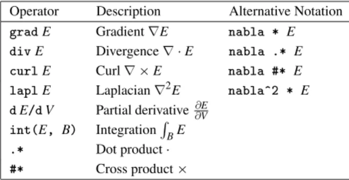
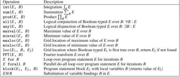
The notational conventions adopted byATMOL allows the PDEs of an atmospheric model to be specified in concise vector notation. Each equa-tion of the set of coupled PDEs of a model is defined using the infix “=” operator. The PDE right-hand sides are arithmetic expressions that can use any of the PDE operators shown in Ta-ble 1. The boundary conditions are given as conditional expressions of the form “EifL”, whereEis an expression andLis a logical ex-pression.
Operator Description Alternative Notation
gradE GradientrE nabla * E
divE Divergencer E nabla .* E
curlE CurlrE nabla #* E
laplE Laplacianr
2E nabla^2 * E
dE/dV Partial derivative@E @V
int(E, B) IntegrationR
BE
.* Dot product
#* Cross product
Table 1.PDE Operators.
Macros can be defined for convenience inAT -MOLusing the “:=” operator. Macros are also used for specifying the components of vectors necessary for the formulation of a model in vec-tor notation. The automatic translation of the equations to scalar form requires the application of the chain-rule to compute symbolic deriva-tives. The chain-rule depends on the coordinate system used by a model. The coordinate sys-tem is set by assigning the coordinates and
coefficientsmacro vectors. For example, the
macro definitions
coordinates := x, y] coefficients := 1, 1].
2.4. Declaration of PDE Operators in ATMOL
New PDE operators can be added to ATMOL. The syntax of an operator declaration is
op:: type(lb..ub)] dimunit]] fieldcoords] :=E].
The operator op is a functional of the form
F(E1:::En). Declarations of the arguments
Eare of the form
arg :: type(var..var)] dim unit] ] field coords]
whereargis a variable name, a wildcard “ ”, or a symbolic expression that serves as a pattern. Thetypes are optional and can be any existing type, including a type variable. When omit-ted, the type of the arguments are assumed to be the same as the result type of operator. The boundslb andubspecify the lower bound and upper bound of the return value of the operator, which can be a symbolic expression using the variables that are part of the value ranges of the arguments expressed with variables var..var. The unitof a variable is a string that specifies the dimensional unit expressed in SI-units and most common derivatives of an expression that calculates the unit from the units of the argu-ments. The coord part specifies dependencies of the variable on the independent variables(
co-ordinates)and the type of grid.
Figure 1 depicts the declarations of pre-defined and most commonly used PDE-operators: de-rivatives, differences, integrals, and midpoint quadratures. The derivative operator “df” is the “inert” variant of thedE/dV partial derivitive operator. The latter operator applies symbolic derivation using the chain-rule to obtain the
df(_ :: float dim U1, _ :: coordinate dim U2) :: float dim (U1/U2).
df(_, _)`grid_overloaded := df_g, df_h, df_c]. df_h(_ :: field x(half), x) :: field x(grid). df_h(_ :: field y(half), y) :: field y(grid). df_h(_ :: field z(half), z) :: field z(grid). df_h(E :: float dim U1, X :: coordinate dim U2)
:: float dim (U1/U2) := (E-E@(X=X-1))/delta X. int(_ :: float dim U1, _ :: domain(coordinate) dim U2)
:: float dim (U1*U2).
int(_, _)`grid_overloaded := mid_g, mid_h, trap]. mid_h(_ :: field x(half), x=_.._) :: field x(grid). mid_h(_ :: field y(half), y=_.._) :: field y(grid). mid_h(_ :: field z(half), z=_.._) :: field z(grid). mid_h(E :: float, X = L .. U :: domain(coordinate))
:: float := sum(E * delta X, X=L..U-1).
Fig. 1.Derivatives, Differences, Integrals, and Quadratures.
derivative ofE, which results in a form that uses the inert “df” operator. Notice that U1 and U2 are unit variables andU1/U2denotes the result-ing dimensional unit of the “df” operator. The “df” derivative operator is overloaded and will be replaced by a concrete operator in the equa-tions. In this case the concrete operators are the finite difference operators “df g”, “df h”, and “df c” that implement three different centered differences depending on the grid location(at
grid points or at half points). The
implementa-tion ofdf his shown in Figure 1. Similarly, the integral “int” operator is overloaded and has three different concrete implementations. The first two are midpoint quadratues and the third is the trapezoidal quadrature.
2.5. Specification of the HIRLAM Model
In this section, we illustrate theATMOL specifi-cation language with realistic examples from the “dynamics” and “physics” parts of theHIRLAM weather forecast system. Due to limitations in space, only the essential subsets of the “dynam-ics” and “phys“dynam-ics” will be shown. The speci-fication and code synthesis of theHIRLAM “dy-namics” and “physics” can be found in27].
The atmospheric models adopted by climate and weather forecast systems are characterized by two main computational components: the
“dynamics” and the “physics”. The
“dynam-ics” is primarily concerned with the fluid dy-namics of the atmosphere, while the “physics” is concerned with the computation of physi-cal parameterizations. In the “dynamics” part of a weather forecast system, the Primitive
Equations 14], which describe the behavior
of the prognostic variables, are solved. In the “physics” part, the aggregate effect of sub-grid processes and of the processes not de-scribed by the PDEs of the primitive equations is computed, such as the effect of solar radi-ation on the atmosphere. Both the “dynam-ics” and “phys“dynam-ics” operate on the same three-dimensional grid that contains a simulated part of the atmosphere.
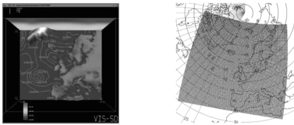
Examples of climate and weather forecast sys-tems with the structure described above are: the HIRLAMnumerical weather forecast system de-veloped by theHIRLAMproject group7, 9], the
Fig. 2.HIRLAMWeather Forecast and Grid Mapping.
developed by the National Center for Atmo-spheric Research (NCAR) 5], and the CSIRO
Atmospheric General Circulation Model devel-oped by theCSIRODivision of Atmospheric Re-search19].
The HIRLAM (HIgh Resolution Limited Area
Model)system9]is a production code written
in Fortran 77. The HIRLAM system comprises a so-called “limited area model” that encom-passes a local part of the globe which is logi-cally of rectangular shape, see Figure 2(forecast
shown with Vis-5D 15]). The “dynamics” of
the HIRLAMsystem is one of the most compu-tationally intensive numerical routines. In the “dynamics” a set of three-dimensional coupled non-linear hyperbolic partial differential equa-tions is solved.
2.5.1. Dynamics
Thesurface pressure tendency equationand the
equation for the auxiliary horizontal wind ve-locity vectorfieldof theHIRLAM“dynamics”9]
are respectively
@ps
@t
= ;
Z 1
0
rVdz (2)
V =
u v
@p
@z
(3)
Eq. (2) describes the tendency of the surface
pressure ps and Eq.(3)describes the auxiliary
horizontal wind velocity vector fieldVwith two componentsuauxandvaux. These PDEs are
dis-cretized by using finite differences on a logically rectangular grid.
Arrangements of variables in the horizontal do-main of atmospheric models were first classi-fied by Arakawa3]. Theu,v, andpfields are
arranged on a staggered Arakawa-C grid as de-picted in Figure 3. Variablepsis located on the
staggered grid at theppoints,uaux andvaux are
located at theuandvpoints, respectively.
Fig. 3.Horizontal Arrangement of Variables on an Arakawa-C Grid.
The first line of the specification of the “dynam-ics” inATMOLshown in Figure 4 declares thex,
% Declare spatial and time dimensions: space (x(i),y(j),z(k)) time t. % Declare grid size variables n, m, and l:
n :: integer(1..infinity) m :: integer(1..infinity) l :: integer(2..infinity). % For convenience, define macros for two grid domains spanning (i,j,k):
atmosphere := i=1..n by j=1..m by k=1..l surface := i=1..n by j=1..m. % Set coordinate system for symbolic derivation with chain-rule:
coordinates := x, y] coefficients := h x, h y]. % Declare the modelfields:
u :: float dim "m/s" field (x(half),y(grid),z(grid)) on atmosphere.
v :: float dim "m/s" field (x(grid),y(half),z(grid)) on atmosphere.
u_aux :: float dim "Pa m/s" field (x(half),y(grid),z(half)) on atmosphere. v_aux :: float dim "Pa m/s" field (x(grid),y(half),z(half)) on atmosphere.
p :: float(0..107000) dim "Pa" field(x(grid),y(grid),z(grid)) monotonic k(+) on atmosphere.
p_s_t :: float dim "Pa/s" field (x(grid),y(grid)) on surface. % Define macro for the horizontal wind velocity vector components:
V := u_aux, v_aux]. % Equations:
p_s_t = -int(nabla .* V, z=1..l). % Eq. (2)
V = u, v] * d p/d z. % Eq. (3)
Fig. 4.Specification of the Surface Pressure Tendency inATMOL.
equations. Field declarations with the Arakawa-C grid arrangements shown in Figure 3 and the equations of the submodel, are specified in CTADELas depicted in Figure 4. Thehalfand gridgrid types are declared inATMOLand are available as pre-defined types.
2.5.2. Physics
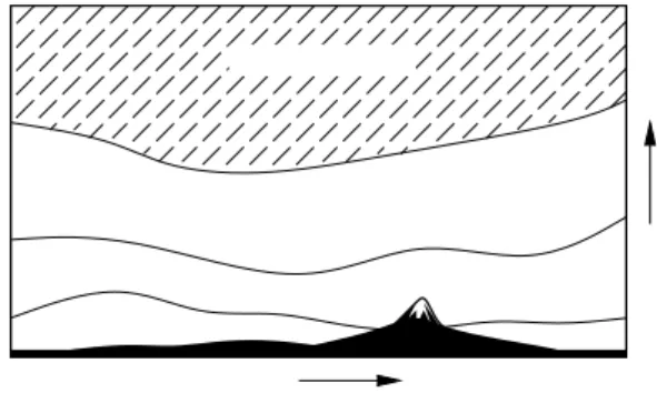
In the so-called cloud routine of the HIRLAM “physics”9], three layers of clouds are
calcu-lated from the “cloudiness” where the layers are defined between four air pressure(p)levels:
surface pressure p= ps,p=200 hPa, p=500
hPa, and p = 800 hPa, respectively, see
Fig-ure 5. InHIRLAM, the vertical coordinate of the global three-dimensional coordinate system is determined by levels of equal air pressure. For each pressure layer, the maximum value in the
Fig. 5.Schematic Illustration of Three Cloud Layers.
vertical direction(z)of the cloudiness
parame-ter(c)defines the low cloud(cl), medium cloud
(cm), and high cloud(ch)parameters. Vertical
ranges of the layers vary with horizontal posi-tion because the air pressurepvaries.
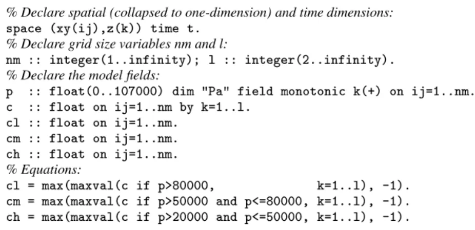
The specification inATMOLis shown in Figure 6. For this model, the two-dimensional horizontal domain has collapsed to one dimension consist-ing ofnm = nmgrid points, which is
con-sistent with the implementation of the physics inHIRLAM. Themaxvaloperator is a reduction operator that returns the maximum value of an expression on a grid, here fork=1..l(see also
Table 3 in Section 3.4). More details can be
found in28].
3. Design and Implementation
% Declare spatial (collapsed to one-dimension) and time dimensions: space (xy(ij),z(k)) time t.
% Declare grid size variables nm and l:
nm :: integer(1..infinity) l :: integer(2..infinity). % Declare the modelfields:
p :: float(0..107000) dim "Pa" field monotonic k(+) on ij=1..nm. c :: float on ij=1..nm by k=1..l.
cl :: float on ij=1..nm. cm :: float on ij=1..nm. ch :: float on ij=1..nm. % Equations:
cl = max(maxval(c if p>80000, k=1..l), -1).
cm = max(maxval(c if p>50000 and p<=80000, k=1..l), -1). ch = max(maxval(c if p>20000 and p<=50000, k=1..l), -1).
Fig. 6.Determination of Cloud Layers inATMOL.
language with which the operational semantics of the model operators is defined. In fact, all built-in PDE-operators, solution methods and algorithms are written inATMOL and provided as pre-defined constructs.
3.1. Levels of Abstraction
ATMOLlanguage constructs can be distinguished at five different levels of abstraction and they present aseparation of concernsfor the imple-mentation of a model. From the highest to the lowest level these are, respectively:
Meta-levelprogramming for symbolic manip-ulationofalgebraic expressionsis one of the key technologies in mathematical software. The user interacts with CTADEL by issuing commands to symbolically translate ATMOL constructs.
Model declarationsare specified inATMOL, as described in the previous sections.
A coordinate-free scalar PDE problemis ob-tained from the model declaration by con-verting vector notation into scalar notation.
The numerical schemes are obtained by ap-plication of the grid type system to coerce continues operators such as partial derivative into discrete operators such as finite differ-ences. Further symbolic manipulation on the results yield optimized numerical solution schemes involving array variables instead of model fields.
Program codeis generated from the optimized schemes.
ATMOLallows specification of a model at mixed abstraction levels. This is useful for models that incorporate lower-level non-PDE-based op-erators, such as the operations in the typical “physics” part of an atmospheric model. A mixed high- and low-level specification can also be used to bypass CTADEL’s automatic transla-tions for (parts of) the model. This gives a
user more control over the implementation of the synthesized solutions by allowing replace-ment of higher-level constructs with lower-level constructs in the model declaration. CTADEL’s translation is deterministic, but optimal transla-tion results are not unique due to the nature of the problem at hand. In some cases, the trans-lation process may produce an intermediate op-timal solution that the user wants to modify to match certain requirements, e.g. based on nu-merical properties.
Model descriptions are translated into code thro-ugh several problem refinement stages. Refine-ment takes place by the application of com-mands to create new intermediate solutions. These commands can be run automatically in a script or they can be applied by a user. Com-mands are available for every refinement stage:
type checkingand coercion of the model
equa-tions and fields, unit analysis to verify the consistency of the model, grid conversionand
discretization of the continuous equations by second-order finite differences and replacement of integrations with midpoint quadratures,
sim-plify the discrete equations, determine array
boundsof discretized variables,eliminate
com-mon-subexpressionsand optimize the
interme-diate code for a target computer architecture,
For-tran 90, HPF (High-Performance Fortran), or
parallel code in Fortran 77 with MPI 13]. To
generate distributed parallel code in Fortran 77 with MPI, CTADELimplements a domain split-ting technique for parallelizing the model 30,
27].
3.2. Expression Syntax for PDEs, Intermediate Constructs, and Program Codes
The syntax ofATMOLis defined as anoperator
precedence grammar1]which provides a
sim-ple and convenient mechanism to dynamically extend the syntax, e.g. while processing prob-lem specification source files. A single operator precedence grammar is used by the CTADEL sys-tem which defines the basic grammar for sym-bolic expressionsE:
E !V jC jEjEjEE j
F (E:::E)j(E:::E)jE:::E]
with variablesV, literal constantsC, functionals
F, prefix operators, postfix operators, and
infix operators. ( )denotes a tuple and ]
denotes a list(possibly empty).
3.3. Type Systems
ATMOLis typed because the simple syntax al-lows too much freedom for the formulation of expressions. For example, it would be syntac-tically legal to embed a Fortran-like program statement in a numerical expression, while such uses should be prohibited. Instead of imposing constraints at the syntactic level, we choose to use type checking to enforce constraints on the formation of well-formed expressions. In ad-dition, type inference and coercion are used to apply dimensional analysis and grid conversion for model verification and translation.
AnATMOLspecification is verified using three different type systems:
Basic typesfor object types, see Table 2. The typescoordinateandindexdistinguish ob-jects that can be used as coordinates and objects that can be used to index a grid. Fortran-like programming constructs are of
thestatementtype.
Unit typesare used in the dimensional analy-sis of a model. The unit types are internally stored as lists of powers of the basic SI-units. For convenience, units are given by the user as strings that are parsed into the internal SI-unit power lists.
Type Description Examples
array(τ, num) array withnumelements of typeτ “A” in “A:i:j”
associative(ρ->σ->τ) associative operator “+”, “*”, and “or”
boolean logical values “false” and “true”
complex IC “complex(1,1/4)”
coordinate a coordinate variable, a subtype offloat “x” and “t”
domain(coordinate) a coordinate domain “x = 0..3/2”
domain(index) an index domain “i = 1..10”
float IR “1.2”
index an index variable, a subtype ofinteger “i”
integer ZZ “7”
interval(integer) integer interval “1..10 step 2”
interval(float) float interval “0.1..5/6 step -0.4”
iteration(coordinate) a coordinate iteration “x = 0..5 step 1/2”
iteration(index) an index iteration “i = 1..10 step k”
list(τ) list ofτ “1,2]”
lvalue(τ) assignableτobject, a subtype ofτ “v” in “v:=5”
range(integer) integer range “1..10”
range(float) float range “0.1..5/6”
rational IQ “1/2”
reference(coordinate) a coordinate reference “x=0.0”
reference(index) an index reference “i=j+1”
statement programming statement “a:=0” and “a:=a+i for i=1..10”
string string “"converged"”
σ->τ operators andλ-abstractions “(a->a+1)”
Grid typesdefine the type of a grid with respect to a given dimension. Grid types are, for ex-ample, staggered finite-difference Arakawa grids 3], finite-volume cells, and spectral
grids.
The three type systems are polymorphic, sup-port subtyping, and allowparameterized types
and type variables. The type systems are sep-arately applied, because the differences in sub-typing and the application of type coercions makes it nearly impossible to integrate them into one type system. Type coercions can take place with user-defined type conversion operations. For example, a user might want to automati-cally convert one type of grid into another by polynomial fitting, which is specified as a con-version operator in the grid type system. The type inference algorithm that implements the three type systems follows a forward/backward
scheme1]and exploits an iterative deepening
search algorithm23]to find the “shortest
con-version path” for the expression which yields an optimal solution(but one that might not be
necessarily unique).
3.4. Aggregate Operators
A novel design choice for ATMOL’s syntax and semantics was made with respect to aggregate operations, which are operations performed on the collection of values of a (sub)grid instead
of on the value of a single grid point. Such choice of design has an important consequence: all of the typical operators used in scientific models, such as integrations, quadratures, re-ductions, scans, sums, FFTs, maxval, maxloc,
etc., and also certain low-level constructs such as Fortran-like do-loops, are expressed with a uniform notation that involves the use of a local scope of a variable in a construct. The effect of our choice of design is comparable to the effect of variable bindings inλ-expressions.
The syntax has the look-and-feel of Maple’s notation of integrals and sums. For example,
“sum(f(i),i=1..10)” has a local binding of a
variable to a range of values. However, the no-tation used in ATMOL is more fundamental as it adopts this convention for all aggregate op-erators that exhibit local bindings of variables, while Maple has an ad-hoc implementation of bindings that is handled by the code associated with integrals and sums.
More formally, ann-ary functionalF,(n> 1),
has alocal scope with variable bindings Bfor argumentsE1:::Ek
;1when the functional is
of the form
F(E1:::Ek ;1
BEk:::En ;1
)
with expressionsEi,i=1:::n;1, for some
k=2:::n, where the binding expressionBis
of the form
B ! B1byBjB1
B1 ! B2 #B1jB2
B2 ! V=Ej(B)
Likewise, a dyadic operatorof the formEB
has alocal scope with variable bindings Bfor expressionE. Theby operator can be viewed
as a sequential construct for composing
bind-ings for multiple variables, while the # operator
Operation Description
int(E, B) IntegrationR
BE
sum(E, B) SummationP
BE
prod(E, B) ProductQ
BE
all(E, B) Logical conjunction of Boolean-typedEoverB:8B:E
any(E, B) Logical disjunction of Boolean-typedEoverB:9B:E
maxval(E, B) Maximum value ofEoverB
minval(E, B) Minimum value ofEoverB
maxloc(E, B) Grid location of maximum value ofEoverB
minloc(E, B) Grid location of minimum value ofEoverB
loc(E1, B, E2) Grid location where Boolean-typedE1is first true overB, returnE2if not found
FFT(E, B) Fourier transformEoverB
E for B Loop over program statementEfor iterationsB
E forall B Parallel do-all loop over program statementEfor iterationsB
block(E1, E2, B) Program statement blockE1with local variablesB(returns value ofE2)
E@B Substitution of variable bindingsBinE
FV V]] := fVgV:dependencies BV V]] :=
FV C]] := BV C]] :=
FV V:=E]] := FV E]] BV V:=E]] := fVg
FV E1;E2]] := (FV E2]]nBV E1]])FV E1]] BV E1;E2]] := BV E1]]BV E2]]
FV E]] := FV E]] BV E]] := BV E]]
FV E]] := FV E]] BV E]] := BV E]]
FV E1 E2]] := FV E1]]FV E2]] BV E1 E2]] := BV E1]]BV E2]]
FV F(E1:::En)]] := Sn
i=1
FV Ei]] BV F(E1:::En)]] := Sn
i=1
BV Ei]]
FV (E1:::En)]] := Sn
i=1
FV Ei]] BV (E1:::En)]] := Sn
i=1
BV Ei]]
FV E1:::En]]] := Sn
i=1
FV Ei]] BV E1:::En]]] := Sn
i=1
BV Ei]]
FV E B]] := (FV E]]nBV B]])FV B]] BV E B]] := BV E]]BV B]]
FV F(E1:::Ek ;1
BEk:::En)]] := ( Sk
;1
i=1
FV Ei]]nBV B]]) Sn
i=k
FV Ei]]FV B]]
BV F(E1:::Ek ;1
BEk:::En)]] := Sk
;1
i=1
FV Ei]] Sn
i=k
BV Ei]]BV B]]
FV B1byB2]] := (FV B1]]nBV B2]])FV B2]] BV B1byB2]] := BV B1]]BV B2]]
FV B1#B2]] := FV B1]]FV B2]] BV B1#B2]] := BV B1]]BV B2]]
FV V=E]] := FV E]] BV V=E]] := fVg
Fig. 7.Free and Bound Variables.
serves as a cross operation orparallelconstruct for binding variables. The scope of bindings is limited to the arguments at the left of the binding expressionB. See Table 3 for examples.
3.5. Free and Bound Variables
The notion of a scope of bindings is formalized by the sets of free and bound variables of an expressionEshown in Figure 7.
In the figure, “V:dependencies” denotes the set
of variables on which V depends as declared by thecoord part of the declaration of V. For example, the variableudeclared in
u :: float dim "m/s"
field (x(half),y(grid),z(grid)) on i=1..n by j=1..m by k=1..l.
has u:dependencies = fxyzg. As a result,
expressions with aggregate operations such as
R1
0 u dxnow make sense, because variableu
de-pends on variablex.
ATMOL’s substitution algorithm replaces free variables in expressions with new values. A substitution is specified with the @-operator, see Table 3. For example, “E@(i=i+1)” re-places all free occurrences of i in E by i+1. This substitution algorithm may rename bound variables in expressions to avoid name clashes, which is comparable toα-conversion as applied byβ-reduction inλ-calculus. The substitution algorithm is frequently used for partial evalua-tion and in the simplificaevalua-tion of expressions.
3.6. Array Variables
The sets of free and bound variables provide a means to check the dimensionality of multi-dimensional objects returned as a result of an expression. The numerical codes of scientific models frequently make use of arrays for stor-age. Synthesis of numerical codes requires in-troduction of(temporary)arrays with proper
el-ement types, dimensionality, and accurate array bounds. This is a non-trivial problem for the im-plementation of numerical schemes in program code. The concept of local bindings and free variables can be used to accurately establish the dimensionality of(temporary) arrays and their
array bounds.
Array Index Analysis The set of free index variables of an expressionE, denotedIVE]],
is defined by
IVE]]:=FVE]]\fVjVis an index variableg
This set describes the index space in which the expression is evaluated, which typically constitutes the grid space of the PDE prob-lem. To generate code forE for numerical evaluation, a loop is constructed that assigns the value ofEto an array variable, sayu:
u:i:j:k := E forall i=1..n by j=1..m by k=1..l
Array Bound Analysis Consider for exam-ple the free index variables of the sym-bolic expression Pl
k=1
AikBkj which is the
set IVsum(A:i:kB:k:jk=1::l) ]] =
fijg Hence, the result can be stored in a
two dimensional array, e.g. Cas in the fol-lowing program fragment
C:i:j := sum(A:i:k*B:k:j, k=1..l) forall i=1..n by j=1..m
which computes the matrix product ofAand
Band assigns the result toC. Adomain in-ference andvalue range propagation6]
al-gorithm based on the substitution alal-gorithm derives the array bounds of array variables in the target code. In the example code frag-ment, the array bounds A:(1..n):(1..l),
B:(1..l):(1..m), andC:(1..n):(1..m)are
derived.
The initial grid domains declared for the fields of a model may be extended by the domain inference to ensure that in the gen-erated codes no references will be made to grid points outside of the domain.
3.7. Dynamic Semantics, Rewrites, and Partial Evaluation
A classification mechanism in CTADEL allows for defining a hierarchy of objects and function-als with algebraic properties. Figure 8 depicts the predefined hierarchy of operator classes. This framework allows for the automatic sim-plification of an operator belonging to a class of objects without the need for specifying individ-ual rewrites for this operator.
Example instances of reduction op are int,
sum, prod, all,any, maxval, and minval. An
operator of the differentiation op class in-herits properties of theself commuting op,
com-muting op, operator, and linear op classes.
Examples are the partial derivativedE/dV op-erator and all finite difference opop-erators. An example integration operator is int and also quadratures are considered integration opera-tors.
An abstract operator abstract op is an over-loaded operator with no implementation. In-stead, the operator will be replaced by a concrete operator from a list ofchoicesthat matches the types used in the context of the operator. Ex-amples are the “df” and “int” operators. CTADEL’s term rewriting system (TRS) is
im-plemented modulo associativity and commuta-tivity(AC), i.e. associativity and commutativity
of operators are implicitly exploited in match-ing rewrite rules. CTADEL’s TRS is also im-plemented modulo operator commuting from operator commuting diagrams. Many oper-ators in scientific models are linear and ex-hibit commuting properties, such as integrals, quadratures, derivatives, finite differences, in-terpolations, sums, FFTs, etc. The commuting relationships between these operators is often graphically described using operator commuta-tivity diagrams. These commuting properties can be declared in ATMOL and are implicitly used by CTADELfor pattern matching in the ap-plication of rewrite rules. For example, when functionalsF0
andF00
are declared to commute, then
F0 (F
00
(EE 00
1:::B 00
:::E 00
m) (4)
E0
1:::B 0
:::E 0
n)
=F 00
(F 0
(EE 0
1:::B 0
:::E 0
n)
E00
1:::B 00
:::E 00
m)
if( Sm
i=1
FVE 00
i]]FVB 00
]])\BVB 0
]] =and
( Sn
i=1
FVE 0
i]] FVB 0
]]) \ BVB 00
]] = and
BVB 0
]] \ BVB 00
]] = . This constraint is
imposed to prevent variable name clashes af-ter the inaf-terchange. For example, the rule to simplify aggregate linear operators of the
lin-ear opclass is
F(E1E2E3:::B:::En) (5)
)E1F(E2E3:::B:::En)
ifF is alinear opandFVE1]]\BVB]] = .
Consider for example the application of rule(5):
sum(sum(f(ij)ii=1::n)j=1::m))
sum(isum(f(ij)j=1::m)i=1::n)
The commuting properties of sums are exploited to interchange the sums when the rule is applied.
3.8. Code Synthesis with Templates
All higher-level functional operators ofATMOL are translated to procedural program code con-structs inATMOLthat resemble Fortran program-ming statements. This intermediate program representation is output in Fortran by a pretty printer. The translation to intermediate code takes place through the application of template definitions for operators. For example, the tem-plate definition of the higher-order “reduce” operator inATMOLis:
reduce(E :: _T, B :: domain(index),
Op :: associative(_T->_T->_T)) :: _T function { reduce := unit_element(Op)
reduce := apply_op(Op, reduce, E) for B }.
Templates are type checked to ensure that the code they contain is statically correct. They are not checked for dimensional units or grid
compatibility, as the templates are applied at a later stage of the translation after discretization through grid inference and coercion. The ex-ample template above uses a type variable T to define the type of the expression, the type of the associative operator, and the type of the result of the operator. This essentially defines the following rewrite rule:
reduce(EB))block(V:=U; (6)
V:=VEforBVV =E:type)
with a new variable V such that V 62 FVE]],
whereU is the unit element of the group with operator. Note that the set of free variables
is not changed by the rewrite. The “block” construct forms a “codelet”. When templates are applied the codelets are combined and op-timized to form a sequence of program state-ments. An example of code generation with templates and optimization of codelets is shown in Figure 9.
The process shown in Figure 9 is lengthy and requires “smart” rules to discover that the dou-ble summation can be performed in one loop. The recognition of opportunities for optimiza-tion at the low-level program code is limited as the code gets more complicated and side-effects get in the way of an accurate analysis. In most cases however, optimizations can be performed at a higher level much more easily and this can have a significant impact on the quality and ef-ficiency of the synthesized codes. For example, consider the rewrite
reduce(reduce(EB1)B2))(7)
reduce(EB1byB2)
reduce(reduce(f(i)i=1::j+)j=1::n+)
) reduce(block(S:=0;S:=S+f(i)for i=1::jSS=integer)j=1::n+)
) block(S:=0;block(S
0
:=0;S 0
:=S 0
+f(i)for i=1::jS:=S+S 0
S 0
=integer)for j=1::nSS=integer)
) block(S:=0;((S
0
:=0;S 0
:=S 0
+f(i)for i=1::j);S:=S+S 0
)for j=1::nSS=integer by S 0
=integer)
) block(S:=0;S:=S+f(i)for i=1::j for j=1::nSS=integer)
INTEGER S S=0
DO 10 j=1,n DO 10 i=1,j S=S+f(i) 10 CONTINUE
which translates multiple reductions into a sin-gle reduction with combined domains and could be applied to the first line of Figure 9. It is easy to verify that this rewrite does not change the set of free variables:
FVreduce(reduce(EB1)B2)]]
=(FVE]]nBVB1]])nBVB2]]
and
FVreduce(EB1byB2)]]
=FVE]]n(BVB1]]BVB2]])
which are identical sets. This rule enables a mapping to code in one step using rule 6:
reduce(f(i)i=1::j by j=1::n+))
block(S:=0;S:=S+f(i)
for i=1::j by j=1::nSS=integer)
This example illustrates the importance of high-level optimizations to avoid potential difficulties with low-level optimizations. The TRS formed by the translation rules is not confluent which is intentional as its purpose is to enable code opti-mizations instead of code normalization which are often contradictory goals.
4. Conclusions
In this paper, we highlighted the features of ATMOL, discussed its design and implementa-tion, and demonstrated the importance of its use in the code generation process of atmospheric models. To our knowledge, the ATMOL lan-guage and the code synthesis approach are novel and is a first attempt to integrate high-level op-timizations with low-level opop-timizations in a unified language and framework for problem refinement and code synthesis.
Acknowledgements
I would like to thank Gerard Cats of the Royal Netherlands Meteorological Institute for his ad-vise. I am grateful to Lex Wolters for his support for the development of CTADEL.
References
1] A. AHO, R. SETHI, AND J. ULLMAN. Compilers:
Principles, Techniques and Tools. Addison-Wesley Publishing Company, Reading MA, 1985.
2] R. L. AKERS, E. KANT, C. J. RANDALL, S. STEIN
-BERG, ANDR. L. YOUNG. SciNapse: A
problem-solving environment for partial differential equa-tions.IEEE Computational Science & Engineering, 4(3):32–42, July/September 1997.
3] A. ARAKAWA ANDV. R. LAMB. A potential
enstro-phy and energy conserving scheme for the shallow water equations.Monthly Weather Review, 109:18– 36, 1981.
4] E. ARGE, A. M. BRUASET, AND H. P. LANGTAN
-GEN,EDITORS.Modern Software Tools for Scientific Computing. Birk¨auser, 1997.
5] L. BATH, J. OLSON,ANDJ. ROSINSKI.User’s Guide
to NCAR CCM2. National Center for Atmospheric Research, Boulder, Colorado, 1992.
6] W. BLUME AND R. EIGENMANN. Demand-driven,
symbolic range propagation. In 8th International
workshop on Languages and Compilers for Parallel Computing, pages 141–160, Columbus, Ohio, USA, August 1995.
7] G. CATS AND L. WOLTERS. The Hirlam project.
IEEE Computational Science & Engineering, 3(4):4–7, 1996.
8] D. DENT, L. ISAKSEN, G. MOZDZYNSKI,
M. O’KEEFE, G. ROBINSON, AND F. WOLLENWE -BER. IFS model: Performance measurements. In
6th ECMWF Workshop on the use of Parallel
Pro-cessors in Meteorology, Reading, UK, November 1994. ECMWF.
9] E. KALL˚ EN´ (ED.). HIRLAM Documentation
Man-ual System 2.5. Norrk¨oping, Sweden, June 1996. Available from SMHI, S–60176.
10] E. GALLOPOULOS, E. HOUSTIS, AND J. R. RICE.
Computer as thinker/doer: Problem-solving
en-vironments for computational science.IEEE Com-putational Science &Engineering, 1:11–23, 1994.
11] D. GANNON, R. BRAMLEY, T. STUCKEY, J. VILLACIS,
J. BALASUBRAMANIAN, E. AKMAN, F. BREG, S. DI -WAN, ANDM. GOVINDARAJU. Developing
compo-nent architectures for distributed scientific problem solving.IEEE Computational Science &Engineer-ing, 1998.
12] JR. G. O. COOK ANDJ. F. PAINTER. ALPAL: A tool to
generate simulation codes from natural descriptions.
Expert Systems for Scientific Computing, 1992.
13] W. GROPP, R. LUSK,ANDA. SKJELLUM.Using MPI,
1994.
14] G. J. HALTINER ANDR. T. WILLIAMS. Numerical
15] W. HIBBARD ANDD. SANTEK. The VIS-5D system
for easy interactive visualization. In IEEE Visual-ization ’90, pages 129–134, 1990.
16] E. N. HOUSTIS, E. GALLOPOULOS, R. BRAMLEY,
ANDJ. R. RICE. Problem-solving environments for computational science. IEEE Computational Sci-ence &Engineering, 4(3):18–21, July/September
1997.
17] E. N. HOUSTIS, J. R. RICE, N. P. CHRISOCHOIDES,
H. C. KARATHANASIS, P. N. PAPACHIOU, M. K.
SAMARTZIS, E. A. VAVALIS, KO-YANGWANG,AND
S. WEERAWARANA. //ELLPACK: A numerical
simulation programming environment for parallel MIMD machines. In 4thACM International
Confer-ence on Supercomputing, pages 96–107, New York, 1990. ACM Press.
18] The Math Works Inc.MATLAB, High-Performance
Numeric Computation and Visualization Software, User’s Guide, 1992.
19] J. L. MCGREGOR, H. L. GORDON, I. B. WATTER
-SON, ANDM. R. DIX. The CSIRO 9-level atmo-spheric general circulation model. Technical paper 26, CSIRO Division of Atmospheric Research, Mordialloc, VIC, 1992.
20] M. F. P. O’BOYLE ANDJ. M. BULL. Expert
program-mer versus parallelizing compiler: A comparative study of two approaches for distributed shared memory.Scientific Programming, 5:63–88, 1996.
21] C. PANCAKE ANDD. BERGMARK. Do parallel
lan-guages respond to the needs of scientific program-mers? IEEE Computing, 23(12):13–23, December
1990.
22] J. R. RICE AND R. F. BOISVERT. Solving Elliptic
Problems Using ELLPACK. Springer Verlag, New York, 1985.
23] E. RICH ANDK. KNIGHT.Artificial Intelligence.
Mc-Graw Hill, New York, 2nd ed edition, 1991.
24] CLEMENSSZYPERSKI. Component Software:
Be-yond Object-Oriented Programming. Addison-Wesley, 1998.
25] P. TU ANDD. PADUA. Gated SSA-based
demand-driven symbolic analysis for parallelizing compilers. In 9thACM International Conference on
Supercom-puting, pages 414–423, New York, July 1995. ACM Press.
26] Y. UMETANI, M. TSUJI, K. IWASAWA, ANDH. HI
-RAYAMA. DEQSOL: A numerical simulation
lan-guage for vector/parallel processors. In B. Ford
and F. Chatelin, editors,Problem Solving Environ-ments for Scientific Computing, Amsterdam, 1987. North-Holland.
27] R. A. VAN ENGELEN. CTADEL: A Generator of
Efficient Numerical Codes. PhD thesis, Leiden Uni-versity, The Netherlands, 1998. ISBN 90-12014-9.
28] R. A.VAN ENGELEN, I. HEITLAGER, L. WOLTERS,
ANDG. CATS. Incorporating application dependent
information in an automatic code generating envi-ronment. In 11thACM International Conference on
Supercomputing, pages 180–187, New York, 1997. ACM Press.
29] R. A.VAN ENGELEN, L. WOLTERS,AND G. CATS.
CTADEL: A generator of multi-platform high
perfor-mance codes for PDE-based scientific applications. In 10th ACM International Conference on
Super-computing, pages 86–93, New York, 1996. ACM Press.
30] R. A.VANENGELEN, L. WOLTERS,ANDG. CATS. The
CTADEL application driver for numerical weather
forecast systems. In A. Sydow, editor, 15thIMACS
World Congress on Scientific Computation, Mod-elling and Applied Mathematics (session: Problem Solving Environments for Scientific Computing), volume 4, pages 571–576, Berlin, Germany, 1997. Wissenshaft &Technik Verlag.
31] R. A.VAN ENGELEN, L. WOLTERS,AND G. CATS.
Tomorrow’s weather forecast: Automatic code generation for atmospheric modeling. IEEE Com-putational Science &Engineering, 4(3):22–31,
July/September 1997.
Received:July, 2001
Revised:October, 2001
Accepted:November, 2001
Contact address:
Robert A. van Engelen Department of Computer Science Florida State University Tallahassee FL 32306-4530 USA e-mail:engelen@cs.fsu.edu
ROBERT VANENGELENreceived his M. Sc.(1994)in Computer
Sci-ence from the University of Utrecht, the Netherlands, and his Ph. D.(1998)in Computer Science from the University of Leiden, the