Large-scale model of mammalian
thalamocortical systems
Eugene M. Izhikevich and Gerald M. Edelman*
The Neurosciences Institute, 10640 John Jay Hopkins Drive, San Diego, CA 92121
Contributed by Gerald M. Edelman, December 27, 2007 (sent for review December 21, 2007)
The understanding of the structural and dynamic complexity of mammalian brains is greatly facilitated by computer simulations. We present here a detailed large-scale thalamocortical model based on experimental measures in several mammalian species. The model spans three anatomical scales. (i) It is based on global (white-matter) thalamocortical anatomy obtained by means of diffusion tensor imaging (DTI) of a human brain. (ii) It includes multiple thalamic nuclei and six-layered cortical microcircuitry based onin vitrolabeling and three-dimensional reconstruction of single neurons of cat visual cortex. (iii) It has 22 basic types of neurons with appropriate laminar distribution of their branching dendritic trees. The model simulates one million multicompartmen-tal spiking neurons calibrated to reproduce known types of re-sponses recorded in vitro in rats. It has almost half a billion synapses with appropriate receptor kinetics, short-term plasticity, and long-term dendritic spike-timing-dependent synaptic plasticity (dendritic STDP). The model exhibits behavioral regimes of normal brain activity that were not explicitly built-in but emerged spon-taneously as the result of interactions among anatomical and dynamic processes. We describe spontaneous activity, sensitivity to changes in individual neurons, emergence of waves and rhythms, and functional connectivity on different scales.
brain models兩cerebral cortex兩diffusion tensor imaging兩oscillations兩 spike-timing-dependent synaptic plasticity
T
he last decade has seen great progress in our understanding of brain dynamics and underlying neuronal mechanisms. Linking these mechanisms to behavior such as perception is facilitated by large-scale computer simulations of anatomically detailed models of the cerebral cortex (1–3). Although these models have stressed microcircuitry and local dynamics, they have not incorporated multiple cortical regions, corticocortical connections, and synaptic plasticity. In the present article, we describe a large-scale model of the mammalian thalamocortical system that includes these components.Spatiotemporal dynamics of the simulation show that some features of normal brain activity, although not explicitly built into the model, emerged spontaneously. The model exhibited self-sustained activity in the absence of any external sources of input. The behavior of the model was extremely sensitive to contributions of individual spikes: adding or removing one spike of one neuron completely changed the state of the entire cortex in⬍0.5 s. Regions of the model brain exhibited collective waves and oscillations of local field potentials in the delta, alpha, and beta ranges, similar to those recorded in humans (4). Simulated fMRI signals exhibited slow fronto-parietal anti-phase oscillations, as seen in humans (5). The shape and connectivity of the model were determined by diffusion tensor imaging (DTI) data for a human brain. Experi-mental data from three species, human, cat, and rat, were incor-porated to build other details of the model.
Model Structure.Here, we review some of the basic assumptions used to construct the model, summarized in Figs. 1–3. A full description is provided insupporting information (SI)Appendix.
For computational reasons, the density of neurons and synapses per mm2of cortical surface was necessarily reduced. Accordingly,
the model neurons have fewer synapses and less detailed dendritic trees than those of real cortical neurons. Although we do not explicitly model subcortical structures other than the thalamus, we do simulate brainstem neuromodulation, including the dopaminer-gic reward system (6, 7) and the cholinerdopaminer-gic activating system. Developmental changes, other than activity-dependent fine-tuning of connectivity due to dendritic STDP, are also not modeled explicitly.
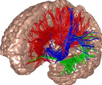
Macroscopic Anatomy.Diffusion tensor imaging (DTI) data derived from magnetic resonance imaging (MRI) of a human brain was used to identify the coordinates of the cortical surface to allocate cell bodies of model neurons at appropriate locations. Conse-quently, the model reflects all areas of the human cortex, the folded cortical structure with sulci and gyri. The DTI data, analyzed using the ‘‘TensorLine’’ algorithm (8, 9), formed the white matter tracts of the model, portions of which are illustrated in Fig. 1, that connect individual neurons in one area with target neurons in other areas. So that neuronal density approached that of animal cortices, spatial scales were reduced by a factor of 4 (so the model cortex
Author contributions: E.M.I. and G.M.E. designed research; E.M.I. performed research; E.M.I. and G.M.E. analyzed data; and E.M.I. and G.M.E. wrote the paper.
The authors declare no conflict of interest.
*To whom correspondence should be addressed. E-mail: [email protected].
This article contains supporting information online atwww.pnas.org/cgi/content/full/ 0712231105/DC1.
© 2008 by The National Academy of Sciences of the USA
Fig. 1. The model’s global thalamocortical geometry and white matter anatomy was obtained by means of diffusion tensor imaging (DTI) of a normal human brain. In the illustration, left frontal, parietal, and a part of temporal cortex have been cut to show a small fraction of white-matter fibers, color-coded according to their destination.
www.pnas.org兾cgi兾doi兾10.1073兾pnas.0712231105 PNAS 兩 March 4, 2008 兩 vol. 105 兩 no. 9 兩 3593–3598
diameter was 40 mm), while relative distances were preserved. The length of the fibers determined axonal conduction delays, which were as long as 20 ms in the model. Because DTI does not presently have sufficient resolution, small bundles of fibers in the human brain were inevitably missed.
Microscopic Anatomy.A summary of simulated gray matter micro-circuitry is presented in Fig. 2. It is based on the detailed recon-struction studies of cat area 17 (visual cortex) by Binzeggeret al. (10), whose nomenclature is adapted here. Depending on the morphology (pyramidal, spiny stellate, basket, non-basket), and the somatic and the target layer, we distinguish eight types of excitatory neurons [p2/3, ss4(L4), ss4(L2/3), p4, p5(L2/3), p5(L5/6), p6(L4), p6(L5/6)] and nine types of inhibitory neurons (nb1, nb2/3, b2/3, nb4, b4, nb5, b5, nb6, b6). SeeSI Appendix for a more detailed explanation, in which we provide the matrix of intercortical con-nectivity and a summary of the magnitudes of laminar axonal spread. Every area of the model cortex had essentially the same microcircuitry as shown in Fig. 2.
The model incorporates specific and nonspecific nuclei of the thalamus, distinguishing two types of excitatory thalamocortical neurons (TCs, TCn) and two types of thalamic inhibitory interneu-rons (TIs, TIn) as well as the inhibitory neuinterneu-rons of the reticular thalamic nucleus (RTN). Axonal arborizations and projection patterns of thalamic neurons were all similar to those reported for LGN (seeSI Appendix).
Branching Dendritic Trees.Each neuron in the model has a somatic compartment and a number of dendritic compartments, with at least one apical compartment per cortical layer (if the dendritic tree
extends to that cortical layer). The exact number of dendritic compartments for each neuron was determined dynamically (seeSI Appendix) during the initialization procedure, maintaining 40 or fewer synapses per compartment.
In most cases, firing of an excitatory presynaptic neuron evoked a local EPSP in the postsynaptic dendritic compartment of⬍10 mV amplitude. Such dendritic EPSPs typically result in a submillivolt EPSP at the somatic compartment because of electrotonic atten-uation of synaptic current. Coincident firing of three or four synapses with maximal conductances in the same compartment can result in a local dendritic action potential (spike), which then can propagate to the soma to evoke a spike or burst response. Similar spikes arriving at different compartments would not be as effective in evoking a somatic response. Conversely, somatic spikes can back-propagate to the dendritic tree evoking dendritic spikes there.
spiny stellate (ss4) cell of layer 4 pyramidal (p) cell non-basket (nb) interneuron basket (b) interneuron local excitatory local inhibitory global cortical cortico-thalamic types of neurons types of synapses
p6(L4) p6(L5/6) p5(L2/3) p5(L5/6) p4 p2/3 cortico-cortical RTN neuron thalamo-cortical (TC) relay cell thalamic interneuron premotor and motor centers specific sensory input specific non-specific reticular thalamic nucleus (RTN) to other cortical areas thalamo-cortical sensory input L1 L2/3 L4 L5 L6 s u m al a ht wm gap junctions g g g g ss4(L4) cifi c e p s-n o n cifi c e p s g g ss4(L2/3) g g g g g g g l a cit r o c-o cit r o c TCs TCn TIs TIn brainstem modulation cortex
Fig. 2. Simplified diagram of the microcircuitry of the cortical laminar structure(Upper)and thalamic nuclei (Lower). Neuronal and synaptic types are as indicated. Only major pathways are shows in the figure. Complete details are provided inSI Appendix. L1-L6 are cortical layers; wm refers to white-matter. Arrows indicate types and directions of internal signals.
200 ms
in vitro (visual cortex) model
25 ms
in vitro (visual cortex) model
pyramidal (p) cell basket (b) interneuron
-60 -80 mV
200 ms
tonic mode burst mode in vitro (LGN) model in vitro (LGN) model
thalamo-cortical (TC) relay cell
short-term synaptic plasticity
50 ms V m 1 in vitro model depression facilitation
A
B
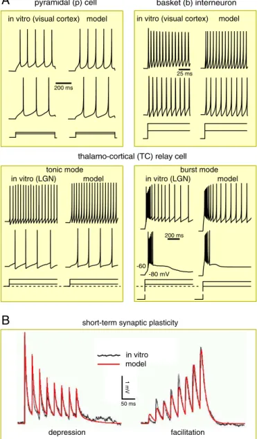
Fig. 3. Firing patterns and short-term synaptic plasticity. (A) Comparisons of four representative firing patterns recordedin vitro(Leftcolumns) and sim-ulated (Rightcolumns) using the phenomenological model (1, 2). Different neuronal types have different values of parameters; seeSI Appendix. (B) Comparison of short-term synaptic plasticity recordedin vitro(black noisy curve; modified from figure 4 of ref. 16) and simulated (red smooth curve) by the model (3).
All such effects are modulated by background excitatory and inhibitory synaptic activity.
Neuronal Dynamics. Spiking dynamics of each neuron and each dendritic compartment are simulated by using the phenomenolog-ical model proposed by Izhikevich (11), which we express here in a dimensional form (12):
Cv˙⫽k共v⫺vr兲共v⫺vt兲⫺u⫹I [1]
u˙⫽a兵b共v⫺vr兲⫺u其 [2]
whereCis the membrane capacitance,vis the membrane potential (in mV),vris the resting potential,vtis the instantaneous threshold
potential,uis the recovery variable (the difference of all inward and outward voltage-gated currents), I is the dendritic and synaptic current (in pA), andaandbare parameters. When the membrane potential reaches the peak of the spike, i.e.,v⬎vpeak, the model fires
a spike (action potential), and all variables are reset according to v
4cand u4u⫹d, wherecanddare model parameters. Notice thatvpeak(typically⬇⫹50 mV) is not a threshold but is a peak of
the spike. The firing threshold in the model (as in real neurons) is not a parameter but a dynamic property that depends on the state of the neuron.
This neuronal model differs from conductance-based Hodgkin-Huxley-type models (13). Instead of reproducing all of the ionic currents, the model was designed to reproduce firing responses; comparein vitrorecordings and simulations in Fig. 3A.
Different neuronal types were given different values of the parameters in Eqs.1and2; seeSI Appendix. Using the nomencla-ture of Connors and Gutnick (14), the excitatory neurons are of RS (regular spiking) type, although some of them also exhibit burst firings evoked by dendritic stimulation; non-basket interneurons in layer 1 (nb1) are of LS type [late spiking (15)]; non-basket cells in the other layers, which morphologically include double-bouquet cells, neurogliaform cells, and Martinotti cells, are of LTS (low-threshold spiking) type; all basket cells are of FS (fast spiking) type; see Fig. 3.
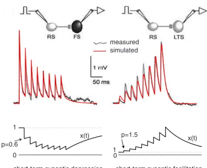
Short-Term Synaptic Plasticity.In the model, the synaptic conduc-tance (strength) of each synapse can be scaled down (depression) or up (facilitation) on a short time scale (hundreds of milliseconds; see e.g., ref. 16) by a scalar factorx. To achieve computational efficiency, this scalar factor, different for each synapse, is modeled by the following one-dimensional equation
x˙⫽共1⫺x兲兾x, if presynaptic spike, thenx 4px. [3] xtends to recover to the equilibrium valuex⫽ 1 with the time constantx, and it is reset by each spike of the presynaptic cell to the
new value px. The parameter p ⬍ 1 decreases xand results in
short-term synaptic depression, whereasp⬎1 results in short-term synaptic facilitation, as we illustrate in Fig. 3B. Different synaptic types have different values ofpandx, provided inSI Appendix.
The total synaptic current at each compartment is the sum of
AMPA, NMDA, GABAA and GABAB currents with standard
kinetics (seeSI Appendix).
Dendritic STDP.The long-term change of conductance (weight) of each synapse in the model is simulated according to spike-timing-dependent plasticity (STDP): The synapse is potentiated or depressed depending on the order of firing of the presynaptic neuron and the corresponding (dendritic) compartment of the postsynaptic neuron (17–20). We use equations in the form provided by Izhikevich (21) so that the synaptic change due to the dendritic STDP develops slowly with time with a rate modulated by dopamine.
Because dendritic compartments can generate spikes indepen-dently from the soma, synapses could be potentiated or depressed
even in the absence of spiking of the postsynaptic cell. All GABAer-gic synapses in the model are nonplastic.
Computer Simulation.The program simulating the model is written in C programming language with MPI and it is run on a Beowulf cluster of 60 3GHz processors with 1.5 GB of RAM each. Most of the simulations were performed with one million neurons, tens of millions of neuronal compartments, and almost half a billion synapses. It takes⬇10 min on the cluster to initialize the model, and one minute to compute one second of simulated data using a sub-millisecond time step.
Results of Simulations
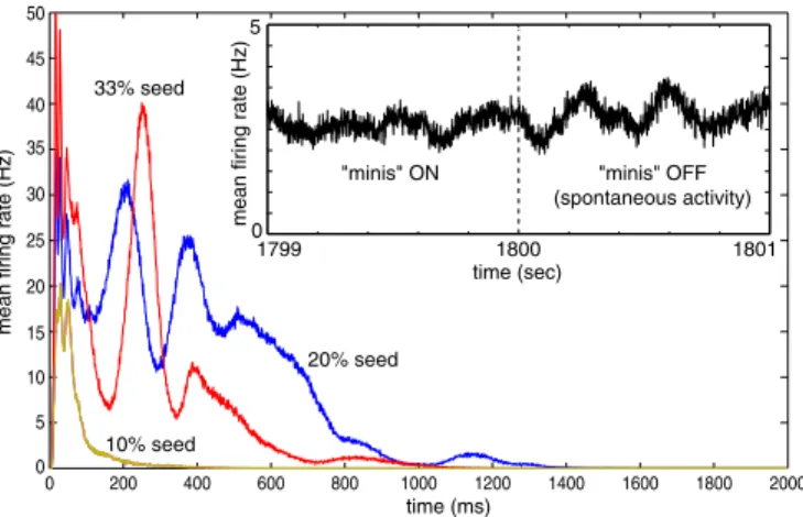
Spontaneous Activity.If there are no spikes fired by the network at the beginning of each simulation, there are no synaptic inputs, and no new spikes, so the network remains completely quiet. To jump-start the network, we introduced a few seed (random) spikes at timet⫽0. Regardless of the number of seed spikes, the initial strength of synaptic connections, or the size of the network (we tested up to 10 million neurons), the network activity died out during the first second, as we illustrate in Fig. 4.
One way to avoid the silent state of a spiking network is to introduce spontaneous synaptic release, called miniature postsyn-aptic potentials, mPSPs or ‘‘minis.’’ Such ‘‘minis,’’ observed bothin vitroandin vivo, are thought to feed neurons with a tonic level of random input necessary to prevent the silent state (22, 23). During the period of the first 30 min of model time (the first 1,800 s in the
Insetof Fig. 4) we simulated one spontaneous (Poissonian) synaptic release per synapse per second and let synaptic plasticity modify the ongoing connectivity. If the minis are turned off during this time, the activity would subside, but the longer they are made to persist, the longer the activity lingers subsequently.
From our previous studies (24, 25) we know that STDP favors synaptic connectivity that results in polychronous activity (i.e., time-locked but not synchronous activity) that can reverberate through the network. Accordingly, turning off minis att⫽1,800 s (Fig. 4) did not silence the network. STDP had fine-tuned the synaptic connectivity in such a way as to allow enough interneuronal action potentials to maintain the global activity. (The network required⬎10,000 neurons to exhibit this property). We ran the model for the next 30 min with ‘‘minis’’ off (i.e., in a noiseless regime) and then used the final state at the end of this 1-h transient period as the initial state for most of the subsequent simulations.
0 200 400 600 800 1000 1200 1400 1600 1800 2000 0 5 10 15 20 25 30 35 40 45 50 5 0 1800 1799 1801 time (sec)
"minis" ON "minis" OFF
(spontaneous activity) ) z H( et ar g nir if n a e m 10% seed 20% seed 33% seed time (ms) ) z H( et ar g nir if n a e m
Fig. 4. Spontaneous activity in the model. Main graph: Activity (shown as mean firing rate in the network) dies out within the first few seconds of simulation regardless of the number of seed spikes introduced at the begin-ning of the simulation. (Inset) The model was simulated with a source of noisy input (spontaneous synaptic release, or ‘‘minis’’) during the first 1,800 s; after the source of noise was turned off, the activity persisted.
Izhikevich and Edelman PNAS 兩 March 4, 2008 兩 vol. 105 兩 no. 9 兩 3595
Each Neuron Matters.Unlike the real brain, where there are many sources of sensory input and neuronal noise, the model exhibited self-sustained activity autonomously in a noiseless environment. To investigate whether the activity is chaotic, we tested for the major hallmark of chaos — the sensitivity of the system to a small perturbation of initial conditions, i.e., the ‘‘butterfly effect’’: Can one spike make a difference? That is, can the state of the entire activity pattern be changed by a firing of a single neuron?
In Fig. 5 we show two traces of total electrical activity (the sum of local-field potentials at every cortical location; seeSI Appendix), starting from the same initial conditions with the only difference being an extra spike of one pyramidal neuron in layer 2/3 of the frontal cortex (manually introduced). Initially, the traces look similar, but after just a few hundred milliseconds, they diverge and result in completely different global activity patterns.
In Fig. 5Lower, we show the difference in the spike rastergrams. As one can see, the extra spike triggered an avalanche of extra spikes (blue dots) or missed spikes (red dots) that eventually spread over the entire network and changed the activity of every neuron. The same effect was seen if we removed a spike in the initial conditions. We did not find any significant difference in the location or type of neuron whose spike was added or removed; on average, it took 400 ms for the perturbed activity trace to diverge one standard deviation from the unperturbed one. The divergence became stronger (faster) as the size of the network increased, although we did not explore this dependence on the size in detail. Similarly, the network was sensitive to the addition of a single somatic EPSP, but it took more time for the perturbation to propagate through the network and often an extra EPSP had no effect on the perturbed neuron or the network.
Brain Rhythms and Waves. Firings of individual pyramidal and non-basket interneurons in the model look Poissonian during
self-sustained spontaneous activity, typically two to three spikes per second. Mean firing rates of basket cells, which are of FS type, were
7 Hz in layer 2/3 and 4, ⬎20 Hz in layer 5 with fluctuations
exceeding 60 Hz, and 8 Hz in layer 6. These cells often had 20- to 25-ms interspike intervals and generated strong local gamma rhythms (40–50 Hz), seen as fast propagating waves inSI Movie 1. However, these rhythms had different phases at different locations. When averaged over a centimeter-size area, they canceled each other and were hardly seen in the power-spectrum of the global electrical activity, consistent with the common experimental ob-servations that gamma rhythms are weaker in EEG and MEG recordings than in LFPs and intracranial EEGs (4).
Although not explicitly built into any type of neurons, prominent low-frequency activity arose in the entire network (Fig. 5). Its predominant frequencies were in the delta (1–3 Hz) and alpha (⬇10 Hz) ranges. The former is typical during mammalian sleep state and the latter during human cortical idling (27).
It is known (11, 25, 26) that simple models of spiking networks can self-organize to exhibit collective delta-, alpha-, and gamma-frequency rhythms. What is remarkable here is that the power spectra at different cortical locations show different predominant rhythms, e.g., strong beta rhythm (⬇20 Hz) in regions correspond-ing to motor and somatosensory areas, even though the cortical microcircuitry at all locations in the model is the same. Thus, the diversity of rhythms in different areas in the model must come largely from differences in the white-matter connectivity between and among cortical areas.
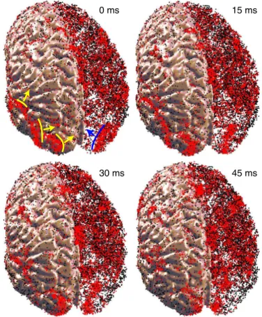
Another striking feature of the model, illustrated in Fig. 6, is that the oscillatory activity was not uniform, but consisted of multiple propagating waves of excitation that spontaneously appeared and disappeared at various locations of the cortex. The waves had a spatial extent of up to a centimeter and a speed of⬇0.1 m/s. These
time (ms) 1000 0 sr et s ar e ki p s f o e c n er eff i d ) A m( s P F L l l a f o m u s b2/3 b4 b5 b6 p2/3 extra spike
Fig. 5. Sensitivity of the model to the addition of a single spike: two simulations starting from the same initial condition, except for a single spike, diverge(Upper)within half a second. (Lower) Shown is the difference of two spike rasters corresponding to the two simulations. Blue or red dots corre-spond to extra or missing spikes, respectively. For the sake of clarity, we show a simulation of a smaller network (100,000 neurons). Horizontal stripes cor-respond to the activity of basket cells, which typically fire with much higher frequency than the other neurons.
0 ms 15 ms
30 ms 45 ms
Fig. 6. Propagating waves in the model. Red (black) dots are spikes of excitatory (inhibitory) neurons. The right hemisphere is transparent to expose the waves inside the cortex (snapshots are fromSI Movie 2).
measures are similar to propagating neocortical waves observedin vitro(28) andin vivoin visual cortex of anesthetized rats (29). They are slower than thosein vivoin primary motor and dorsal premotor cortices of monkeys (30) and in turtle visual cortex (31).
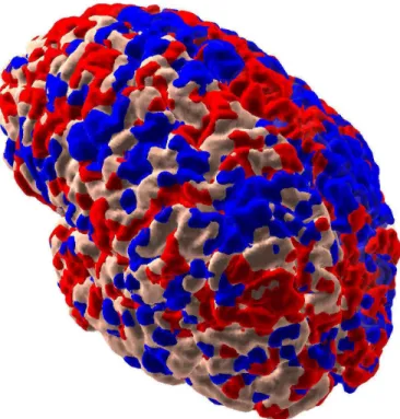
Functional Connectivity.As suggested by studies of human subjects (5), we can analyze the resting state correlations of the simulated signals corresponding to fMRI (BOLD signals) on the slow time scales of minutes. Following Foxet al. (5), we collect signals (seeSI Appendix) at each voxel of the cortical surface, low-pass filter them between 0.1 and 0.01 Hz, and then correlate the results with a seed region corresponding to posterior cingulate. Regions positively and negatively correlated with the seed region are depicted in red and blue, respectively, in Fig. 7. Our results resemble those seen in experimental brain studies of human (5) and theoretical studies (32), indicating that the resting state of the mammalian brain on this scale consists of multiple anticorrelated functional clusters.
Discussion
One way to deepen our understanding of how synaptic and neuronal processes interact to produce the collective behavior of the brain is to develop large-scale, anatomically detailed models of the mammalian brain. We started with the thalamocortical system because it is necessary for human consciousness. Cur-rently, we are at the stage of calibrating and further validating the model by determining to what extent its activity is similar to that recorded in the mammalian cortex after receipt of various input signals.
Even in the absence of external input, the distribution of firing rates among various types of neurons is similar to that recordedin
vivo: pyramidal neurons fire just a few spikes per second with the lowest firing rate observed in layer 2/3, whereas basket cells fire tens of spikes per second with the highest firing rate in layer 5 (33). Individual neurons exhibit somatic and dendritic spikes, forward-and back-propagation of spikes along the dendritic trees, forward-and spike-timing-dependent plasticity that is coupled to the dendritic compartments rather than to the somatic spikes. The model spon-taneously generated rhythms and propagating waves (Fig. 6) that had frequency distributions, spatial extents, and propagation ve-locities similar to those observed in mammalianin vivorecordings. In a fashion similar to human data, the simulated fMRI signal exhibited slow oscillations with multiple anticorrelated functional clusters (Fig. 7).
The computer model allowed us to perform experiments that are impossible (physically or ethically) to carry out with animals. For example, we put the model into the noiseless regime to demonstrate that it can produce self-sustained autonomous activity. We perturbed a single spike (34, 35) in this regime (out of millions) and showed that the network completely reorga-nized its firing activity within half a second. It is not clear, however, how to interpret this sensitivity in response to pertur-bations (Fig. 5). On one hand, one could say that this sensitivity indicates that only firing patterns in a statistical sense should be considered, and individual spikes are too volatile. On the other hand, one could say that this result demonstrates that every spike of every neuron counts in shaping the state of the brain, and hence the details of the behavior, at any particular moment. This conclusion would be consistent with the experimental observa-tions that microstimulation of a single tactile afferent is detect-able in human subjects (36), and that microstimulation of single neurons in somatosensory cortex of rats affects behavioral responses in detection tasks (37).
After development of a detailed, more complete brain model, one may simulate the effect of structural perturbations, such as lesions, strokes, and tumors, on the global dynamics, and com-pare the results with animal or human EEG/MEG data. By using DTI of patients with Alzheimer’s disease, Parkinson’s disease, or other neurological and psychiatric disorders, one may investigate how the connectivity alone modifies brain dynamics. Changing the neuronal parameters to simulate the effect of various pharmacological agents, one may study the effect of drugs (including addictive drugs) on the dynamics of the model to aid design of new therapeutic strategies against neurological disor-ders. By simulating the effect of cholinergic modulatory systems, one may induce sleep oscillations into the model and study the dynamics of the sleep state and its effect on synaptic plasticity, learning, and memory. Knowing the state of every neuron and every synapse in such a model, one may analyze the mechanisms involved in neural computations with a view toward develop-ment of novel computational paradigms based on how the brain works. Finally, by reproducing the global anatomy of the human thalamocortical system, one may eventually test various hypoth-eses on how discriminatory perception and consciousness arise.
ACKNOWLEDGMENTS.Data files of cortical microcircuitry were kindly provided
by Tom Binzegger, Rodney J. Douglas, and Kevan A. C. Martin (Eth Zurich, Zurich, Switzerland). The simulations were performed by using two MRI DTI data files, one of the brain of the first author (E.M.I.) and the other provided by Gordon Kindlmann (Scientific Computing and Imaging Institute, University of Utah), and Andrew Alexander [W. M. Keck Laboratory for Functional Brain Imaging and Behavior, University of Wisconsin-Madison (www.sci.utah.edu/gk/DTI-data/ )]. Jeff Krichmar, Botond Szatmary, Douglas Nitz, and Niraj Desai provided useful comments. The authors are especially grateful to Dr. Joe Gally, who suggested many important improvements to the manuscript. This work was supported by the Neurosciences Research Foundation and by National Science Foundation Grant CCF-0523156.
1. Lumer ED, Edelman GM, Tononi G (1997) Neural dynamics in a model of the thalamo-cortical system. I. Layers, loops and the emergence of fast synchronous rhythms.Cereb Cortex7:207–227.
2. Lumer ED, Edelman GM, Tononi G (1997) Neural dynamics in a model of the thalamo-cortical system. II. The role of neural synchrony tested through perturbations of spike timing.Cereb Cortex7:228 –236.
Fig. 7. Intrinsic correlations of fMRI signal between the seed cortical region in a location corresponding to posterior cingulate [data not shown; see Foxet al. (5)] and other regions in the model brain. Red (blue) voxels correspond to positive (negative) correlations (⬎1 standard deviation of correlations of all voxels to the seed region). The right hemisphere is transparent so that inside voxels are visible.
Izhikevich and Edelman PNAS 兩 March 4, 2008 兩 vol. 105 兩 no. 9 兩 3597
3. Markram H (2006) The blue brain project.Nat Rev Neurosci7:153–160.
4. Nunez PL, Srinivasan R (2006)Electric Fields of the Brain: The Neurophysics of EEG
(Oxford Univ Press, New York), 2nd Ed.
5. Fox MD,et al. (2005) The human brain is intrinsically organized into dynamic, anticor-related functional networks.Proc Natl Acad Sci USA102:9673–9678.
6. Schultz W (2007) Reward.Scholarpedia2:1652. 7. Schultz W (2007) Reward signals.Scholarpedia2:2184.
8. Weinstein D, Kindlmann G, Lundberg E (1999) Tensorlines: Advection-diffusion based propagation through diffusion tensor fields.Proceedings of the IEEE Conference on Visualization ’99: Celebrating Ten Years(IEEE Computer Society Press, Los Alamitos, CA), pp 249 –253.
9. Mori S, van Zijl PCM (2002) Fiber tracking: Principles and strategies–a technical review.
NRM Biomed15:468 – 480.
10. Binzegger T, Douglas RJ, Martin KAC (2004) A quantitative map of the circuit of cat primary visual cortex.J Neurosci24:8441– 8453.
11. Izhikevich EM (2003) Simple model of spiking neurons.IEEE Trans Neural Netw
14:1569 –1572.
12. Izhikevich EM (2007)Dynamical Systems in Neuroscience: The Geometry of Excitability and Bursting(MIT Press, Cambridge, MA).
13. Skinner FK (2006) Conductance-based models.Scholarpedia1:1408.
14. Connors BW, Gutnick MJ (1990) Intrinsic firing patterns of diverse neocortical neurons.
Trends Neurosci13:99 –104.
15. Chu Z, Galarreta M, Hestrin S (2003) Synaptic interactions of late-spiking neocortical neurons in layer 1.J Neurosci23:96 –1002.
16. Beierlein M, Gibson JR, Connors BW (2003) Two dynamically distinct inhibitory net-works in layer 4 of the neocortex.J Neurophysiol90:2987–3000.
17. Levy WB, Steward O (1983) Temporal contiguity requirements for long-term associa-tive potentiation/depression in the hippocampus.Neuroscience8:791–797. 18. Gerstner W, Kempter R, van Hemmen JL, Wagner H (1996) A neuronal learning rule for
sub-millisecond temporal coding.Nature383:76 –78.
19. Markram H, Lubke J, Frotscher M, Sakmann B (1997) Regulation of synaptic efficacy by coincidence of postsynaptic APs and EPSPs.Science275:213–215.
20. Bi GQ, Poo MM (1998) Synaptic modifications in cultured hippocampal neurons: Dependence on spike timing, synaptic strength, and postsynaptic cell type.J Neurosci
18:10464 –10472.
21. Izhikevich EM (2007) Solving the distal reward problem through linkage of STDP and dopamine signaling.Cereb Cortex17:2443–2452.
22. Timofeev I, Grenier F, Bazhenov M, Seijowski TJ, Steriade M (2000) Origin and slow cortical oscillations in deafferented cortical slabs. Cereb Cortex10:1185– 1199.
23. Muresan RC, Savin C (2007) Resonance or Integration? Self-sustained dynamics and excitability of neural microcircuits.J Neurophysiol97:1911–1930.
24. Izhikevich EM, Gally JA, Edelman GM (2004) Spike-timing dynamics of neuronal groups.Cereb Cortex14:933–944.
25. Izhikevich EM (2006) Polychronization: Computation with spikes.Neural Comput
18:245–282.
26. Ananthanarayanan R, Modha DS (2007) Anatomy of a Cortical Simulator, Supercom-puting 07: Proceedings of the ACM/IEEE SC2007 Conference on High Performance Networking and Computing(Association for Computing Machinery, New York, NY). 27. Bazhenov M, Timofeev I (2006) Thalamocortical oscillations.Scholarpedia1:1319. 28. Bao W, Wu J-Y (2003) Propagating wave and irregular dynamics: Spatiotemporal
patterns of cholinergic theta oscillations in neocortexin vitro.J Neurophysiol90:333– 341.
29. Xu W, Huang X, Takagaki K, Wu J-Y (2007) Compression and reflection of visually evoked cortical waves.Neuron55:119 –129.
30. Rubino D, Robbins KA, Hatsopoloulos NG (2006) Propagating waves mediate infor-mation transfer in the motor cortex.Nat Neurosci9:1549 –1557.
31. Prechtl JC, Cohen LB, Pesaran B, Mitra PP, Kleinfeld D (1997) Visual stimuli induce waves of electrical activity in turtle cortex.Proc Natl Acad Sci USA94:7621–7626. 32. Honey CJ, Kotter R, Breakspear M, Sporns O (2007) Network structure of cerebral cortex
shapes functional connectivity on multiple time scales.Proc Natl Acad Sci USA
104:10240 –10245.
33. Swadlow HA (1994) Efferent neurons and suspected interneurons in motor cortex of the awake rabbit: Axonal properties, sensory receptive fields, and subthreshold syn-aptic inputs.J Neurophysiol71:437– 453.
34. Latham PE, Roth A, Hausser M, London M (2006) Requiem for the spike?Soc Neurosci Abstr32:432.12.
35. Banerjee A (2006) On the sensitive dependence on initial conditions of the dynamics of networks of spiking neurons.J comput Neurosci20:321–348.
36. Vallbo ÅB, Olsson KÅ, Westberg K-G, Clark FJ (1984) Microstimulation of single tactile afferents from the human hand: Sensory attributes related to unit type and properties of receptive fields.Brain107:727–749.
37. Houweling AR, Brecht M (2008) Behavioural report of single neuron stimulation in somatosensory cortex.Nature451:65– 68.
SI Appendix 2
We simulated a large-scale thalamocortical network consisting of one million neurons and up to one billion synaptic connections. Parameters of the network are scaled to preserve ratios found in the mam-malian thalamocortical system. The white matter anatomy of the model is reconstructed from human diffusion tensor imaging (DTI) data using fiber-tracktography methods. The gray-matter anatomy con-sists of 5 cortical layers with microcircuitry of a “generic primary sensory area” and specific, non-specific, and reticular thalamic nuclei. The model has 12 types and numerous subtypes of neurons with multi-compartment dendritic trees; synapses with AMPA, NMDA, GABAA, GABAB, and gap-junction kinetics;
axonal lengths and conduction delays; synaptic short-term depression and facilitation; synaptic long-term spike-timing-dependent plasticity (STDP); and neuromodulation derived from the brainstem dopaminergic reward system. The parameters of the model are taken from the published literature, mostly on cat area 17 and lamina A of dorsal thalamus. In some cases, a number of arbitrary but justifiable choices had to be made.
As compared to real cortex, the model has a scaled down density of neurons and synapses per mm2
of cortical surface. Model neurons have scaled down number of synapses and impoverished dendritic trees in comparison with real cortical neurons. Moreover, we do not model subcortical structures other than the thalamus. We do not model developmental changes other than that reflected in activity-dependent fine-tuning of connectivity.
Most simulations were performed with one million neurons, though a variant of the model was simulated with 1011 neurons and almost one quadrillion synapses, which corresponds to the full size of the human brain. Movies of the simulation are available on the first author website (http://www.izhikevich.com).
1
Anatomy
1.1 Microcircuitry
Neurons in the model are either excitatory (glutamatergic, red in Fig. 8) or inhibitory (GABAergic, blue or green in Fig. 8). We adapt the nomenclature of [1] and distinguish the following types of cortical excitatory neurons:
p2/3 pyramidal neurons in L2/3
ss4(L4) spiny stellate neurons in L4 that project to L4 ss4(L2/3) spiny stellate neurons in L4 that project to L2/3
p4 pyramidal neurons in L4
p5(L2/3) pyramidal neurons in L5 that project to L2/3 p5(L5/6) pyramidal neurons in L5 that project to L5/6
p6(L4) pyramidal neurons in L6 that project to L4 p6(L5/6) pyramidal neurons in L6 that project to L5/6
Pyramidal neurons exhibit regular spiking (RS) firing patterns (Connors and Gutnick 1990), but can also exhibit chattering (CH, or fast rhythmic bursting FRB) pattern or intrinsically bursting (IB) pattern, which we describe in detail below.
We distinguish two types of cortical GABAergic (inhibitory) interneurons b basket interneuron, all layers
SI Appendix 3 spiny stellate cell of layer 4 pyramidal cell non-basket (nb) interneuron basket (b) interneuron local excitatory local inhibitory global cortical cortico-thalamic types of neurons types of synapses p6(L4) p6(L5/6) p5(L2/3) p5(L5/6) p4 p2/3 cortico-cortical RTN neuron thalamo-cortical (TC) relay cell thalamic interneuron premotor and motor centers specific sensory input specific non-specific reticular thalamic nucleus (RTN) cortex to other cortical areas thalamo-cortical sensory input brainstem modulation L1 L2/3 L4 L5 L6 th a la m u s wm gap junctions g g g g ss4(L4) n o n -s p e c if ic s p e c if ic g g ss4(L2/3) g g g g g g g c o rt ic o -c o rt ic a l 1mm .55 1.12 .15 1.0 .15 .55 .15 .15 .15 .3 1.12 .4 .15 .15 .5 .4 p2/3 p4 ss4(L4) ss4(L2/3) 1mm .15 .4 .3 .5 .25 p5(L2/3) .5 1.0 .15 p5(L5/6) .15 p6(L5/6) 1.0 .15 .15 .15 p6(L4) b nb .5 .2 TCs .8 TCn .8 TCs TCn TIs TIn p6 p5 sensory input RTN cell 1mm .25 .5 TI .25 TC .25 .15 .15 .4 L1 L2/3 L4 L5 L6 L1 L2/3 L4 L5 L6 thalamus RTN b2/3 .5 .15 .2
Figure 8: Simplified diagram of thalamocortical microcircuit. Only the most significant or numerous con-nections are shown; see Fig. 9 for details. Self-synapses denote synaptic concon-nections within the populations. Bold lines denote pathways carrying more than 30% of synapses to a particular target.
SI Appendix 4
Basket cells have fast spiking (FS) firing patterns [2]. Non-basket interneurons morphologically include double-bouquet cells, neurogliaform cells, and Martinotti cells [1], and they can exhibit LTS (low-threshold spiking, [3]), LS (latent spiking), RSNP (regular spiking non-pyramidal neurons) or BSNP (burst spiking non-pyramidal neurons) firing patterns [4, 5], and a diversity of other patterns [6], as we explain the next section. In the model, basket interneurons in L4, L5, and L6 have axons confined within a single cortical layer, whereas basket cells in L2/3 and non-basket interneurons may have axons spanning several layers [7, 8].
We distinguish three thalamic nuclei with three cell types:
TCs thalamocortical relay neurons in specific nucleus TCn thalamocortical relay neurons in non-specific nucleus
TIs thalamic interneurons in specific nucleus TIn thalamic interneurons in non-specific nucleus
RTN GABAergic neurons in the reticular thalamic nucleus
We do not make the distinction between X and Y thalamocortical relay neurons [9]. TC and RTN cells exhibit regular spiking or bursting patterns depending on the holding potential.
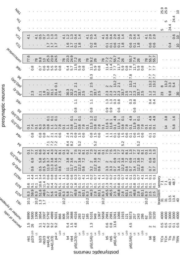
The relative distribution (percentage) of neuronal types in the model is given in the first column in Fig. 9. It is based on the following published data: The relative number of cortical neurons in different layers in the primary visual cortex was given by [1], Fig. 6). Consistent with earlier studies, they found that inhibitory neurons form approximately 20% of all neurons. The relative number of basket and non-basket cells is consistent with earlier studies (Fig. 4 of [10], Fig. 1 of 5). The relative number of neurons in the thalamic nuclei is not known. Peters and Payne [11] report 350,000 thalamocortical fibers per 11,000,000 neurons in L4 of area 17 [1], resulting in a ratio of 1/30, which is consistent with other observations [12]. Assuming one such fiber per TC cell, we derive the number of TC cells as a fraction of L4 neurons. Winer and Larue [13] report 20% of interneurons in LGN of rats, cats, and monkeys, but different percentages in other nuclei. We assume here that exactly 20% of neurons in the specific and non-specific thalamic nuclei are inhibitory interneurons. Not knowing the number of RTN neurons, we take it to be the same as the number of TC neurons in each nucleus. Notice that the majority of neurons in the model are in L2/3, L4 and L6.
Making three-dimensional reconstructions of 39 single neurons and thalamic afferents in cat primary visual cortex (area 17), Binzegger et al. [1] characterized the distribution of all synapses formed on each neuronal type at each cortical layer, see Fig. 7 in their paper. The authors kindly provided us with their data files, which were used to obtain the cortical part of the table in Fig. 9. We treat 95% of the unidentified asymmetrical (excitatory) synapses in L1-L6 as coming from other cortical areas (corticocortical) and 5% as coming from the non-specific thalamic nucleus. We treat the unidentified symmetrical (inhibitory) synapses as coming from non-basket cells. Converting the absolute values into percentages, we assign synapses in the model with the distribution in shown in the table in Fig. 9.
The table also reflects the relative distribution of synapses in the thalamus, which is based on the numbers found in the A-laminae of the LGN of the cat. van Horn et al. [14] found that TC neurons in LGN receive 7.1% synapses from sensory (retinal) fibers, 62% excitatory synapses from cortex (L5 and L6) and brainstem (divided equally between the two, see Erisir et al. 1997 and 30.9% GABAergic synapses. Thalamic interneurons receive 48.7% synapses from sensory fibers, 24.4% GABAergic synapses, and the
SI Appendix 5 presynaptic neurons postsynaptic neurons brainstem sensory nb1 p2/3 b2/3 nb2/3 ss4(L4) ss4(L2/3) p4 b4 nb4 p5(L2/3) p5(L5/6) b5 nb5 p6(L4) p6(L5/6) b6 nb6 TCs TCn TIs TIn TRN corticcortical percent of cells number of synapses nb1 1.5 p2/3 L2/3 L1 26 b2/3 3.1 nb2/3 4.2 ss4(L4) 9.2 ss4(L2/3) 9.2 p4 L4 L2/3 L1 9.2 b4 5.4 nb4 1.5 p5(L2/3) L5 L4 L2/3 L1 4.8 p5(L5/6) L5 L4 L2/3 L1 1.3 b5 0.6 nb5 0.8 p6(L4) L6 L5 L4 L2/3 13.6 p6(L5/6) L6 L5 L4 L2/3 L1 4.5 b6 2 nb6 2 TCs 0.5 TCn 0.5 TIs 0.1 TIn 0.1 TRN 0.5 8890 10.1 6.3 0.6 1.1 . . 0.1 . . 0.1 . . . . . . . . 4.1 . . . 77.6 5800 . 59.9 9.1 4.4 0.6 6.9 7.7 . 0.8 7.4 . . . 2.3 . . 0.8 . . . . . . 1306 10.2 6.3 0.1 1.1 . . 0.1 . . 0.1 . . . . . . . . 4.1 . . . 78 3854 1.3 51.6 10.6 3.4 0.5 5.8 6.6 . 0.8 6.3 . . . 2.1 . . 0.7 . 0.5 . . . 9.8 3307 1.7 48.6 11.4 3.3 0.5 5.5 6.2 . 0.8 5.9 . . . 1.8 . . 0.6 . 0.7 . . . 13 5792 . 2.7 0.2 0.6 11.9 3.7 4.1 7.1 2 0.8 0.1 . . 32.7 . . 5.8 1.7 1.3 . . . 25.3 4989 . 5.6 0.4 0.8 11.3 3.8 4.3 7.2 2.1 1.1 0.1 . . 31.1 . . 5.5 1.7 1.3 . . . 23.9 5031 . 4.3 0.2 0.6 11.5 3.6 4.2 7.2 2.1 1.2 0.1 . . 31.4 0.1 . 5.9 1.7 1.3 . . . 24.5 866 . 63.1 5.1 4.1 0.6 7.2 8.1 . 0.6 7.8 . . . 2.5 . . 0.8 . . . . . . 806 10.2 6.3 0.1 1.1 . . 0.1 . . 0.1 . . . . . . . . 4.1 . . . 78 3230 . 5.8 0.5 0.8 11 3.8 4.2 8.4 2.4 1.1 . . . 30.3 . . 5.4 1.6 1.2 . . . 23.3 3688 . 2.7 0.2 0.6 11.7 3.6 4 8.2 2.3 0.8 0.1 . . 32.2 . . 5.7 1.7 1.3 . . . 24.9 4316 . 45.9 1.8 0.3 3.3 2 7.5 . 0.9 11.7 1 0.8 1.1 2.3 2.1 . 11.5 0.1 0.4 . . . 7.2 283 . 2.8 0.1 0.7 12.2 3.8 4.2 5.2 1.5 0.8 0.1 . . 33.7 . . 5.9 1.8 1.4 . . . 26 412 . 63.1 5.1 4.1 0.6 7.2 8.1 . 0.6 7.8 . . . 2.5 . . 0.8 . . . . . . 185 10.2 6.3 0.1 1.1 . . 0.1 . . 0.1 . . . . . . . . 4.1 . . . 78 5101 . 44.3 1.7 0.2 3.2 2 7.3 . 0.8 11.3 1.2 0.8 1.1 2.3 2.5 0.3 11.3 0.2 0.5 . . . 9.2 949 . 2.8 0.1 0.7 12.2 3.8 4.2 5.2 1.5 0.8 0.1 . . 33.7 . . 5.9 1.8 1.4 . . . 26 1367 . 63.1 5.1 4.1 0.6 7.2 8.1 . 0.6 7.8 . . . 2.5 . . 0.8 . . . . . . 5658 10.2 6.3 0.1 1.1 . . 0.1 . . 0.1 . . . . . . . . 4.1 . . . 78 2981 . 45.5 2.3 0.2 3.3 2 7.5 . 1.1 11.6 1 0.9 1.3 2.3 2 . 11.4 0.1 0.4 . . . 7.2 2981 . 45.5 2.3 0.2 3.3 2 7.5 . 1.1 11.6 1 0.9 1.3 2.3 2 . 11.4 0.1 0.4 . . . 7.2 3261 . 2.5 0.1 0.1 0.7 0.9 1.3 . 0.1 0.1 4.9 . 0.3 1.2 13.2 7.7 7.7 0.6 2.9 . . . 55.7 1066 . 46.8 0.8 0.3 3.4 2.1 7.7 . 0.6 11.9 1 0.6 0.8 2.3 2.1 . 11.7 0.1 0.4 . . . 7.4 1915 . 2.8 0.1 0.7 12.2 3.8 4.2 5.2 1.5 0.8 0.1 . . 33.7 . . 5.9 1.8 1.4 . . . 26 121 . 63.1 5.1 4.1 0.6 7.2 8.1 . 0.6 7.8 . . . 2.5 . . 0.8 . . . . . . 5573 . 2.5 0.1 0.1 0.7 0.9 1.3 . 0.1 0.1 4.9 . 0.3 1.2 13.2 7.8 7.8 0.6 2.9 . . . 55.7 257 . 46.8 0.8 0.3 3.4 2.1 7.7 . 0.6 11.9 1 0.6 0.8 2.3 2.1 . 11.7 0.1 0.4 . . . 7.4 243 . 2.8 0.1 0.7 12.2 3.8 4.2 5.2 1.5 0.8 0.1 . . 33.7 . . 5.9 1.8 1.4 . . . 26 286 . 63.1 5.1 4.1 0.6 7.2 8.1 . 0.6 7.8 . . . 2.5 . . 0.8 . . . . . . 62 10.2 6.3 0.1 1.1 . . 0.1 . . 0.1 . . . . . . . . 4.1 . . . 78 3220 . 2.5 0.1 0.1 0.7 0.9 1.3 . 0.1 0.1 4.9 . 0.4 1.2 13.2 7.7 7.7 0.6 2.9 . . . 55.7 3220 . 2.5 0.1 0.1 0.7 0.9 1.3 . 0.1 0.1 4.9 . 0.4 1.2 13.2 7.7 7.7 0.6 2.9 . . . 55.7 4000 31 . 7.1 . . . . . . . . . . 23 8 . . . . 5 . 25.9 . 4000 31 . 7.1 . . . . . . 14 3.8 . . . 13.2 . . . . . 5 25.9 . 3000 13.5 . 48.7 . . . . . . . . . . 9.8 3.3 . . 0.4 . 24.4 . . . 3000 13.4 . 48.7 . . . . . . 5.8 1.6 . . . 5.4 . . . 0.6 . 24.4 . . 4000 40 . . . . . . . . . . . . 30 . . . 10 10 . . 10 .
Figure 9: Distribution of neuronal types and synapses in the model. Each row represents a single postsy-naptic neuron of a certain type. Multiple compartments, if they exist, are indicated. Each element in a row represents the percentage of synapses of a particular type to that neuron. The most significant connections are shown in Fig. 8. Shaded regions denote plastic connections.
SI Appendix 6
rest are from cortex and brainstem. Since there are four types of cortical pyramidal neurons projecting to thalamus, we assume that the distribution of cortico-thalamic synapses in the thalamus is proportional to the relative distribution of the cortical neurons. We assume that RTN neurons are qualitatively similar to TC neurons with respect to the number of brainstem synapses, cortico-thalamic synapses, etc.
Notice that the table has very few zero (empty) entries; for the sake of clarity, we depict only the most significant or numerous connections in Fig. 8. Bold lines in the figure denote projections from p2/3 and p6(L4) that carry the majority of synaptic input (more than 30% each) to their targets. The proportion of thalamocortical synapses is small, but the synapses are quite strong, as we discuss in the next section.
Generalizing the interneuron circuitry of L4 of barrel somatosensory cortex of rats ([3]; Michael Beierlein and Jay Gibson, personal communication) we assume that the connectivity of interneurons is the same in all cortical layers: There are gap-junction (electrical) synapses among neurons of the same type at each layer and no gap junctions between neurons belonging to different types. Landisman et al. [15] report gap junctions among RTN neurons in mice and rats, but no chemical synapses. In contrast, [16] and [17] report GABAergic synapses in the same neurons. We include both types of synapses in the model of the thalamic reticular nucleus. Hughes et al. [18] report gap junctions among TC relay neurons. Since no evidence exists of any chemical synapses among the neurons [12], only electrical synapses among TC cells are modeled in this study.
Typical axonal arborizations of various neuronal types are illustrated in Fig. 8, lower-left. The magni-tudes of the laminar axonal spread of cortical neurons are based on the macaque striate cortex data of [19] and [20], which are consistent with cat area 17 data of [1]. Thalamic neurons are from [21] and reticular neurons are from [22] and [15]. Sur et al. [23] report the diameter of cat retino-geniculate arborizations to be 0.15 mm for X-type and 0.3 mm for Y-type, whereas [24] report slightly larger estimates. We take the radius of sensory fibers in the model to be 0.2 mm. Murphy and Sillito [25] report the spread of L6 cortico-thalamic arborizations to be 0.5 mm with some fibers spreading as much as 1.5 mm. We assume that the radius of thalamic arborization of all cortical axons is 0.4 mm. Jones ([12], Fig.3.9) reports the spread of thalamocortical fibers to be around 0.4 mm for X-type and 0.8 mm for Y-type with multiple synaptic clusters. Since we do not distinguish the types, we take the larger number and keep in mind that there will be activity-dependent pruning.
Yellow circles in Fig. 8 with indicated radii (mm) denote the initial axonal spans used in the model. The synaptic density decays linearly from the center of the circle to a zero value at the edge.
1.2 White Matter Anatomy (After Human DTI)
The gross anatomy of long-range corticocortical connections in the model is based on the anatomy of the human brain obtained via anatomical MRI and DTI scans. Neuronal bodies are allocated randomly on the cortical surface, whose coordinates were obtained from anatomical MRI. Local-circuit connectivity is established according to Fig. 8 and table in Fig. 9. The axons that exit the gray matter and enter the white matter are directed according to the ”TensorLine” method ([26, 27]) applied to human DTI scans; see Fig. 1 of the main text. Once the axon re-enters the gray matter (in some distal part of the cortex), it ramifies according to the distances in Fig. 8.
Axons of each pyramidal neuron in layer 2/3 in the model bifurcates into ipsilateral and contralateral axons. The former are continued according to the DTI data, and the latter project to the mirror locations
SI Appendix 7
in the contralateral hemisphere. Because human hemispheres are not symmetrical, the target point for the axon is found on the contralateral hemisphere that is closest to the mirror location of the neuron.
Each thalamocortical neuron in the non-specific thalamic nuclei projects to a random location on cortex. The specific nuclei are assumed to have the form of two hemispheres and thalamocortical neurons there project roughly topographically to corresponding locations in the cortex. To deliver visual, auditory, or somatosensory signals, we stimulate corresponding neurons in the specific thalamic nuclei that project to the visual, auditory, and somatosensory areas of the cortex.
To have a sufficiently large density of neurons per mm2 of cortical surface, we scaled down the entire
structure by a factor of 4. That is, we assumed that the cortex is 40mm wide, i.e., it can be embedded within a sphere with diameter of 40mm. The length of the traced fibers is used to estimate the axonal conduction delays as follows: For corticocortical connections, we assume that the axonal conduction velocity is 1m/s for myelinated fibers and 0.1 m/s for non-myelinated fibers (28–30]. The cortex is assumed to have 1 mm width, so a delay from layer 6 to layer 1 could be as large as 10ms. Delays via myelinated (in white matter) and non-myelinated (in gray matter) fibers are added to find the total conduction delay. The delays from layer 5 to thalamus are taken to be 1 ms and from layer 6 to thalamus are taken to be 20 ms. Delays from specific thalamocortical neurons are taken to be 1 ms. Delays from non-specific thalamocortical cells are determined according to the length of the axonal fiber. If the resulting conduction delay of any neuron is longer than 20 ms, it is reduced to exactly 20 ms to have an efficient implementation algorithm (this number is a parameter in the model, and it can be easily changed; we used 20ms for all our simulations). Sensory input to the model is delivered via stimulation of the thalamocortical neurons (TCs) projecting to the appropriate primary sensory cortex (appropriate sensory modality). In particular, to deliver auditory, visual, or somatosensory stimulation, we inject brief pulses of current into TCs neurons in the MGN, LGN, and VPN nuclei of thalamus.
2
Dynamics
The large-scale model consists of various types of multi-compartmental neurons with active dendrites, synaptic transmission with AMPA, GABA, and NMDA kinetics, and short-term and long-term synaptic plasticity with dopaminergic modulation.
2.1 Neuronal Dynamics
Spiking dynamics of each neuron (and each dendritic compartment) were simulated using the phenomeno-logical model proposed by Izhikevich [31]. The model has only 2 equations and 4 dimensionless parameters that could be explicitly found from neuronal resting potential, input resistance, rheobase current, and other measurable characteristics ([32], chapter 8). We present the model in a dimensional form so that the membrane potential is in millivolts, the current is in picoamperes and the time is in milliseconds:
Cv˙ = k(v−vr)(v−vt)−u+I (1)
˙
u = a{b(v−vr)−u} (2)
whereC is the membrane capacitance, vis the membrane potential (in mV),vr is the resting potential,vt
SI Appendix 8
voltage-gated currents),I is the dendritic and synaptic current (in pA)
I(t) =−Idendr−Isyn
as explained below,aand bare parameters. When the membrane potential reaches the peak of the spike, i.e.,v > vpeak, the model is said to fire a spike, and all variables are reset according tov ←candu←u+d,
wherecanddare parameters. Notice thatvpeak(typically around +50 mV) is not a threshold but is rather
a peak of the spike; the firing threshold in the model (as in real neurons) is not a parameter but a dynamic property that depends on the state of the neuron.
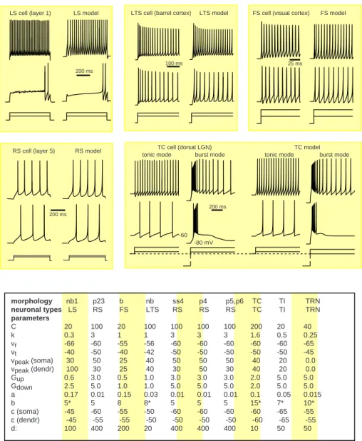
Depending on the values of the parameters, the model could be tuned to reproduce firing dynamics of every known cortical, thalamic, and hippocampal neuron ([32). We illustrate some of the firing patterns in Fig. 10 using injected pusles of somatic current (see Fig. 8.17 in [32] for in vivo-like input). It is different from the Hodgkin-Huxley-type models in the sence that it reproduces the responses, and not the ionic currents, of biological neurons.
Each neuron has a somatic compartment and a set of dendritic compartments. The number of dendritic compartments of a neuron in each cortical layer is at least S∗scale/M whereS is the number of synapses the neuron receives in the layer (see Fig. 9), scale= 0.05 is the scale-down factor when we simulate fewer than 1011 neurons, and the parameter M = 40 is the maximal number of synapses per compartment. The dendritic current at each compartment consists of the currents coming from the down (”mother”) compartment (zero for somatic compartments) and up (”daughter”) compartments (zero for terminal compartments)
Idendr=Gdown(V −Vdown) +X
up
Gup(V −Vup)
with the values of the conductancesGup and Gdown provided in Fig. 10.
2.2 Synaptic Dynamics
We model synaptic dynamics in a fashion similar to that by Izhikevich et al. [33] with the exception that we use a simpler and more efficient model for short-term synaptic plasticity, and spike-timing-dependent plasticity (STDP) is considered to be modulated by dopamine.
Short-Term Synaptic Plasticity. We assume that the synaptic conductance (strength) of each synapse can be scaled down (depression) or up (facilitation) on a short time scale (hundreds of milliseconds) by a scalar factor x. This scalar factor, different for each presynaptic cell, is modeled by the following one-dimensional equation
˙
x= (1−x)/τx , x←px when presynaptic neuron fires. (3)
That is,xtends to recover to the equilibrium valuex= 1 with the time constantτx, and it is reset by each
spike of the presynaptic cell to the new value px. Any value p < 1 decreases x and results in short-term synaptic depression, whereasp >1 results in short-term synaptic facilitation, as we illustrate in Fig. 11.
SI Appendix 9
200 ms
RS cell (layer 5) RS model
LTS cell (barrel cortex) LTS model
100 ms 25 ms
FS cell (visual cortex) FS model
200 ms
LS cell (layer 1) LS model
-60 -80 mV
200 ms
TC cell (dorsal LGN) TC model
tonic mode burst mode tonic mode burst mode
morphology nb1 p23 b nb ss4 p4 p5,p6 TC TI TRN neuronal types LS RS FS LTS RS RS RS TC TI TRN parameters C 20 100 20 100 100 100 100 200 20 40 k 0.3 3 1 1 3 3 3 1.6 0.5 0.25 vr -66 -60 -55 -56 -60 -60 -60 -60 -60 -65 vt -40 -50 -40 -42 -50 -50 -50 -50 -50 -45 vpeak (soma) 30 50 25 40 50 50 50 40 20 0.0 vpeak (dendr) 100 30 25 40 30 50 30 40 20 0.0 Gup 0.6 3.0 0.5 1.0 3.0 3.0 3.0 2.0 5.0 5.0 Gdown 2.5 5.0 1.0 1.0 5.0 5.0 5.0 2.0 5.0 5.0 a 0.17 0.01 0.15 0.03 0.01 0.01 0.01 0.1 0.05 0.015 b 5* 5 8 8* 5 5 5 15* 7* 10* c (soma) -45 -60 -55 -50 -60 -60 -60 -60 -65 -55 c (dendr) -45 -55 -55 -50 -50 -50 -50 -60 -65 -55 d: 100 400 200 20 400 400 400 10 50 50
Figure 10: Comparison between in vitro recordings of various neurons and their simulations in the large-scale model. Different neuronal types are modeled by the same equations 1 and 2 but with different
choice of parameters. ∗: Dendritic compartments of the LS neuron are modeled as a passive compartment
˙
v= (−Idendr−Isyn)/250. For LTS neurons, the recovery variable is kept below the value of 670; that is, if
u >670, thenu= 670. For TI neurons, if u >530, thenu= 530. For TC and TRN neurons, the value b
SI Appendix 10
0 1
0 1
short-term synaptic depression short-term synaptic facilitation
x(t) x(t)
p=0.6
p=1.5 measured simulated
neuronal types (to) p,ss (RS) b (FS) nb (LS, LTS)
(from)
p,ss (RS) tx=150, p=0.6 tx=150, p=0.6 tx=100, p=1.5
b (FS) tx=150, p=0.6 tx=150, p=0.6
TC tx=150, p=0.7 tx=200, p=0.5
x'=(1-x)/tx , x px when presynaptic neuron fires
Figure 11: Short-term synaptic depression and facilitation is modeled by the one-dimensional equation
3 with two parameters, τx and p. Top: comparison of experimentally measured (Fig. 4 from [3]) and
simulated synaptic dynamics. Bottom: values of parameters used in the large-scale model. Other synaptic connections, e.g., from nb (LTS) cells, are assumed not to have short-term plasticity.
SI Appendix 11
Synaptic Kinetics. The total synaptic current at each compartment is simulated as
Isyn = gAMPA(v−0) +gNMDA [(v+ 80)/60] 2
1 + [(v+ 80)/60]2(v−0)
+gGABAA(v+ 70) +gGABAB(v+ 90) + Igap
where v is the postsynaptic membrane potential, and the subscript indicates the receptor type. Each conductance g(here we omit the subscript for the sake of clarity) has first-order linear kinetics
˙
g=−g/τ
withτ =5, 150, 6, and 150 ms for the simulated AMPA, NMDA, GABAAand GABAB receptors,
respec-tively [34, 33].
The ratio of NMDA to AMPA receptors was set to be uniform at a value of 1 for all excitatory neurons. Thus, each firing of an excitatory neuron increases gAMPA and gNMDA by xc, where c is the synaptic
conductance (synaptic weight) and x is the short-term depression/potentiation scaling factor as above. Similarly, the value of GABAA to GABAB receptors is taken to be 1 for all inhibitory synapses.
The gap-junction (electrical synapse) current
Igap= X
i∈neighbors
gi(v−vi)
has conductance decaying with the distance from the neuronal soma to the neighboring neuroni. Evaluation of the gap-junction currents is extremely costly from a computational point of view, since they need to be evaluated pair-wise for all neurons at all time steps, and most of the results presented in the paper were performed with gi = 0 (unless mentioned otherwise).
Dopamine-modulated dendritic STDP. The conductance (weight) of each synapse in the model is simulated according to spike-timing-dependent plasticity (STDP): The synapse is potentiated or depressed depending on the order of firing of the presynaptic neuron and the corresponding (dendritic or somatic) compartment of the postsynaptic neuron (35, 36, 37, 38). We use equations in the form provided by 32 so that STDP could be modulated by dopamine. In particular, we use the parameters A+ = 1, A− = 2,
τ+=τ−= 20 ms (see [39 or 40]) so that the depression area of the STDP function is twice as large as the potentiation area.
Since dendritic compartments can generate spikes independently from the soma, synapses could be potentiated or depressed even in the absence of spiking of the postsynaptic cell. We keep the synaptic conductance within the range [0, smax], where smax is 10.0 if the presynaptic cell is of pyramidal (p) or spiny stellate (ss) type, 20.0 if the presynaptic cell is of thalamocortical (TC) type, 6.0 if the presynaptic cell is of basket (b) type, 4.0 if the presynaptic cell is of non-basked (nb) type, and 5.0 if the presynaptic cell is of thalamic inhibitory (TI) or reticular thalamic nucleus (RTN) type. All GABAergic synapses in the model are assumed to be non-plastic and their conductance is fixed at the value of 4.0. The initial values of the glutamatergic synapses are random drawn from the uniform distribution on the interval [0,6], and then they evolve according to STDP.
SI Appendix 12
In most cases, firing of an excitatory presynaptic neuron can evoke a local EPSP in the dendritic compartment of the postsynaptic cell of less than 10 mV amplitude, which typically results in submillivolt EPSP at the somatic compartment due to the electrotonic attenuation of synaptic current. Coincident firing of three or four synapses with the maximal conductancesin the same compartment may result in a local dendritic spike, which then could propagate to the soma and evoke a spike or burst response there. Such spikes arriving at different compartments would not be as effective in evoking the somatic response.
3
Intracranial EEG
We assume that the intracranial EEG (iEEG) at any cortical location is the sum of all extracellular currents generated by nearby neurons within a sphere of radius of 1.5 mm, so it is essentially the sum of local field potentials. These currents are mostly the intracellular currents flowing across vertically aligned apical dendrites of pyramidal cells. The basal dendrites of pyramidal cells and the dendritic trees of the other types of neurons are not aligned; they may generate many strong currents, but the currents flow at random directions and thereby cancel each other.
4
Simulated fMRI/BOLD
We simulate fMRI/Blood Oxygenation Level Dependent (BOLD) signal [41] at each region (voxel) as the sum of all synaptic activity (all synaptic conductances) of all neurons within the region
˙
y= (total synaptic conductance)−y/500.
Thus, we assume that the major source for metabolic demand in the model is the synaptic transmission.
Acknowledgment
Data files of cortical microcircuitry were kindly provided by Tom Binzegger, Rodney J. Douglas, and Kevan A.C. Martin. The simulations were performed using two MRI DTI data files, one of the brain of the first au-thor (Eugene M. Izhikevich) and the other provided by Gordon Kindlmann at the Scientific Computing and Imaging Institute, University of Utah, and Andrew Alexander, W. M. Keck Laboratory for Functional Brain Imaging and Behavior, University of Wisconsin-Madison (http://www.sci.utah.edu/~gk/DTI-data/). Materials and methods necessary to reproduce the results are available upon request.
References
1. Binzegger T., Douglas R.J., Martin K.A.C. (2004) A Quantitative Map of the Circuit of Cat Primary Visual Cortex. Journal of Neuroscience, 24:8441–8453.
2. Connors B.W and Gutnick M.J. (1990) Intrinsic firing patterns of diverse neocortical neurons. Trends in Neuroscience, 13:99–104.
SI Appendix 13 3. Beierlein M., Gibson J.R., and Connors B.W. (2003) Two Dynamically Distinct Inhibitory Networks
in Layer 4 of the Neocortex. Journal of Neurophysiology, 90:2987–3000.
4. Kawaguchi Y. (1995) Physiological Subgroups of Nonpyramidal Cells with Specific Morphological Characteristics in Layer II/III of Rat Frontal Cortex. Journal of Neuroscience, 15:2638–2655.
5. Kawaguchi Y. and Kubota Y. (1997) GABAergic Cell Subtypes and their Synaptic Connections in Rat Frontal Cortex. 7:476–486.
6. Markram H., Toledo-Rodriguez M., Wang Y., Gupta A., Silberberg G., and Wu C. (2004) Interneu-rons of the Neocortical Inhibitory System. Nature Reviews Neuroscience, 5:793–807.
7. Kubota Y. and Kawaguchi Y. (2000) Dependence of GABAergic Synaptic Areas on the Interneuron Type and Target Size. Journal of Neuroscience. 20:375–386.
8. Xiang Z., Huguenard J.R., and Prince D.A. (1998) Cholinergic Switching Within Neocortical In-hibitory Networks. Science, 281:985–988.
9. Sherman S.M. and Guillery R.W. (2004) Thalamus. In Shepherd G.M. (Ed.) The Synaptic Organi-zation of the Brain. Oxford University Press.
10. Amitai Y., Gibson J.R., Beierlein M., Patrick S.L., Ho A.M., Connors B.W. (2002) The Spatial Di-mensions of Electrically Coupled Networks of Interneurons in the Neocortex. Journal of Neuroscience, 22:4142–4152.
11. Peters A. and Payne B.R. (1993) Numerical relationships between geniculocortical afferents and pyramidal cell modules in cat primary visual cortex. Cerebral Cortex, 3:69–78
12. Jones, E.G. (1985) The Thalamus, New York: Plenum Press.
13. Winer J.A. and Larue D.T. (1996) Evolution of GABAergic circuitry in the mammalian medial geniculate body. PNAS 93:3083–3087.
14. van Horn S.C., Erisir A. and Sherman S.M. (2000) Relative Distribution of Synapses in the A-Laminae of the Lateral Geniculate Nucleus of the Cat. J. Compar. Neurology, 416:509–520.
15. Landisman C.E., Long M.A., Beierlein M., Deans M.R., Paul D.L., and Connors B.W. (2002) Elec-trical Synapses in the Thalamic Reticular Nucleus. Journal of Neuroscience, 22:1002–1009.
16. Zhang S.J., Huguenard J.R., Prince D.A. (1997) GABAA Receptor-Mediated Cl− Currents in Rat
Thalamic Reticular and Relay Neurons. JOurnal of Neurophysiology, 78:2280–2286.
17. Sohal V.S., Huntsman M.M., and Huguenard J.R. (2000) Reciprocal Inhibitory Connections REgulate the Spatiotemporal Properties of Intrathalamic Oscillations. Journal of Neuroscience, 20:1735–1745.
18. Hughes SW, Blethyn KL, Cope DW, and Crunelli V. (2002) Properties and origin of spikelets in thalamocortical neurones in vitro. Neuroscience 110:395–401
SI Appendix 14 19. Blasdel G.G., Lund J.S., Fitzpatrick D. (1985) Intrinsic Connections of Macaque Striate Cortex:
Axonal Projections of Cells Outside Lamina 4C. Journal of Neuroscience, 5:3350–3369.
20. Fitzpatrick D., Lund J.S., Blasdel G.G. (1985) Intrinsic Connections of Macaque Striate Cortex: Afferent and Efferent Connections of Lamina 4C. Journal of Neuroscience, 5:3329–3349.
21. Yen C.T., Conley M., Hendry .S.H.C., Jones E.G. (1985) The Morphology of Physiologically Identified GABAergic Neurons in the Somatic Sensory Part of the Thalamic Reticular Nucleus in the Cat. JOurnal of Neuroscience, 5:2254–2268.
22. Cox C.L., Huguenard J.R., and Prince D.A. (1997) Nucleus reticularis neurons mediate diverse inhibitory effects in thalamus. PNAS, 94:8854–8859.
23. Sur M., Esguerra M., Garraghty P.E., Kritzer M.F., and Sherman S M. (1987) Morphology of Phys-iologically Identified Retinogeniculate X- and Y-Axons in the Cat. Journal of Neurophysiology, 58:1–32.
24. Bowling D.B. and Michael C.R. (1994) Terminal Patterns of Single, Physiologically Characterized Optic Tract Fibers in the Cat’s Lateral Geniculate Nucleus. Journal of Neuroscience, 4:198–216.
25. Murphy P.C. and Sillito A.M. (1996) Functional Morphology of the Feedback Pathway from Area 17 of the Cat Visual Cortex to the Lateral Geniculate Nucleus. Journal of Neuroscience, 16:1180–1192.
26. Weinstein D., Kindlmann G., Lundberg E. (1999) Tensorlines: advection-diffusion based propagation through diffusion tensor fields. IEEE Proceedings of the conference on Visualization’99. p. 249 - 253
27. Mori S. and van Zijl P.C.M. (2002) Fiber tracking: principles and strategies - a technical review. NRM in Biomedicine, 15:468-480.
28. Swadlow H. A. (1991) Efferent neurons and suspected interneurons in second somatosensory cortex of the awake rabbit: receptive fields and axonal properties. J Neurophysiol 66: 1392-1409
29. Swadlow H. A. (1992) Monitoring the excitability of neocortical efferent neurons to direct activation by extracellular current pulses. J Neurophysiol 68: 605–619
30. Swadlow H.A. (1994) Efferent Neurons and Suspected Interneurons in Motor Cortex of the Awake Rabbit: Axonal Properties, Sensory receptive Fields, and Subthreshold Synaptic Inputs. Journal of Neurophysiology, 71: 437-453.
31. Izhikevich E. M. (2003) Simple Model of Spiking Neurons. IEEE Transactions on Neural Networks, 14:1569-1572
32. Izhikevich E. M. (2007) Dynamical Systems in Neuroscience: The Geometry of Excitability and Bursting. The MIT Press
33. Izhikevich E.M., Gally J.A., and Edelman, G.M. (2004) Spike-Timing Dynamics of Neuronal Groups. Cerebral Cortex, 14:933-944
SI Appendix 15 34. Dayan P. and Abbott L. F. (2001) Theoretical Neuroscience: Computational and Mathematical
Modeling of Neural Systems. The MIT Press, Cambridge, MA
35. Levy W.B. and Steward O. (1983) Temporal contiguity requirements for long-term associative po-tentiation/depression in the hippocampus. Neuroscience, 8:791–797
36. Gerstner W., Kempter R., van Hemmen J. L., Wagner H. (1996) A neuronal learning rule for sub-millisecond temporal coding Nature, 383: 76 - 78
37. Markram, H., Lubke, J., Frotscher, M. and Sakmann, B. (1997). Regulation of synaptic efficacy by coincidence of postsynaptic APs and EPSPs. Science, 275, 213-215.
38. Bi, G.Q., and Poo, M.M. (1998). Synaptic modifications in cultured hippocampal neurons: depen-dence on spike timing, synaptic strength, and postsynaptic cell type. J. Neurosci. 18, 10464-10472.
39. Izhikevich E.M. and Desai N.S. (2003) Relating STDP to BCM. Neural Computation 15:1511-1523
40. Izhikevich E.M. (2006) Polychronization: Computation With Spikes. Neural Computation,18:245-282