Chapter 4
Dimensionless expressions
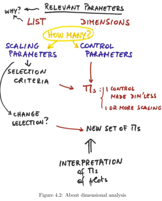
Dimensionless numbers occur in several contexts. Without the need for dy-namical equations, one can draw a list (real or tentative) of physically rel-evant parameters, and use the Vaschy-Buckingham theorem to construct a shorter dimensionless list. Dimensionless expressions are the required tool to compare data from different experiments (e.g. parachute data in water), leading to the recommendation that all data should be plotted in dimen-sionless form. This is generally covered at the undergraduate level, and a few points of interpretation are added here. The same dimensionless expres-sions are obtained from dynamical equations, when available: the meaningful dimensionless numbers are ratios of terms in various equations, measuring their relative importance. This can be used to approximate the equations rationally, by dropping small (dynamically inactive) terms. One notable ex-ception is when the small parameter is the coefficient of the highest-order derivative in the equation...
4.1
Dimensional analysis
This material is assumed known from undergraduate courses: fill in any gaps (and practice) by consulting undergraduate textbooks from the library re-serve. We will review the procedure (same for all problems) with one familiar example as illustration. Occasional features not shown in the example will be mentioned for reference.
1. The list of parameters:
(a) This step determines the eventual solution, and several attempts may be necessary to identify the list that makes sense of the data. The list should be sufficiently complete to account for the physics of the flow, but not to the point of introducing unnecessary com-plications: trial-and-error, from the simpler to the more elaborate, is sensible. The list is a reflection of individual insight and of the profession’s expertise.
(b) Example: We will work with fully developed flow in a circular pipe. The list of parameters includes: flow parameters (pressure drop per unit length dp/dx, average speed V), pipe configuration (diameterDor cross-sectional areaA, not independent of course), and material properties (fluid density ρ and viscosity µ).
δp/L V D ρ µ
not included: surface roughness; etc.
(c) If some relations are known (e.g. between velocity, cross-sectional area and volume flow rate), the corresponding parameters are not independent, and one of them can be eliminated from the list for each such relation. Also, in this problem, we start from the pres-sure drop per unit length of pipe, rather than prespres-sure drop and overall length as separate variables: the assumed proportionality between them is a valuable insight (try solving without it and note the differences!)
2. Primary dimensions:
(a) ‘Dimensions’ are more general than ‘units’; e.g. meter, foot and mile and micron are units relevant to the dimension of length. In general, there are 3 dimensions (M, L, T for mass, length and time respectively - other combinations can be used) for mechanical problems (some dimensions may be irrelevant in some problems, e.g. mass in simple pendulum), and then one each for thermal problems (θ for temperature), chemical, electromagnetic and ra-diation problems. The maximum is 7, use only as many as needed, 3 or 4 are most common in mechanical engineering problems. (b) Example:
The dimensions of each of the problem parameters are listed. When not obvious, use a simple relation (e.g. pressure is force
4.1. DIMENSIONAL ANALYSIS 105
per unit area, force is mass times acceleration, etc.)
δp/L V D ρ µ M L−2 T−2 LT−1 L M L−3 M L−1 T−1
3. Select the scaling parameters:
(a) This is the next critical step. One must select as many scaling parameters (those that serve as dimensional yardsticks for all oth-ers) as there are independent dimensions. The scaling parame-ters must contain all dimensions in such a way that one cannot make a dimensionless expression between them; options include the selection of the simplest expressions, and/or the exclusion of the parameters you wish to solve for (see interpretation, below), called ‘control parameters’
(b) Example:
In this instance, we want to know about pressure drop, so we set it aside if possible; speed and diameter are simple and would be selected; then we need mass as a dimension, and density is simpler so we select it. 3 dimensions, 3 scaling parameters:
δp/L V D ρ µ
M L−2T−2 LT−1 L M L−3 M L−1T−1
↑ ↑ ↑
Pressure drop and viscosity are our control parameters in this case. (c) Occasionally, some groupings of dimensions (e.g. LT−1) may have
to serve as a single dimension: go back one step and start again. 4. Non-dimensionalize each of the control parameters
(a) Then, repeat the following procedure for each of the control pa-rameters in turn: take a parameter, multiply it by powers of the scaling parameters, and adjust the exponents to make the expres-sion dimenexpres-sionless. (b) Example: Π1 = δp LV a Dbρc 1 =M L−2 T−2 LaT−aLbMcL−3c 1 =M1+cT−2−a L−2+a+b−3c
c=−1 a =−2 b= 1 Π1 = δpD LρV2 Similarly we find Π2 = µ ρV D (4.1)
Always check these results! Always double-check the initial di-mensions! Expect for standard expressions (e.g. Re) to come out. (c) The procedure involves a system of linear equations for the ex-ponents of each scaling parameter. The proof of the Vaschy-Buckingham theorem (see undergrad text) is based on the rank of the corresponding matrices.
5. The result
(a) The idea is that there is a relation between the parameters in the initial list; since any relation, reflecting fundamental laws and phenomenology too complicated to unravel analytically, must be dimensionally correct, it can be rearranged as a relation between dimensionless parameters. Since there are fewer of these, the re-lation is much simpler.
(b) Example:
In our case, we have reduced the problem of friction in pipe flows to the relation Π1 = F(Π2) δp L = ρV2 D ψ(ReD) δp ρg = V2 2g L Df(ReD)
where F, ψ and f are as-yet unspecified functions. We recognize the Reynolds number, and we recover the familiar definition of the Darcy friction factor in the Moody diagram. Note that the relation involves an unknown function, not necessarily a proportionality. (c) It is customary to express the pressure drop in terms of the height
4.1. DIMENSIONAL ANALYSIS 107
of pressure measurement, notto the friction in the pipe, hence it should not be included in the initial list of parameters and serves only for the presentation of the result.
6. Rearrangements and interpretation
(a) The procedure explained above gives a relation between the di-mensionless control parameters. Given a result (e.g. reduced ex-perimental data) in the form Π1 = F(Π2,Π3, ...), you can
deter-mine their meaning by noting that the scaling parameters appear in more than one of the Πs, whereas the control parameters ap-pear in only one each.
However, you may wish to present the results differently: say you want to know how the pressure drop depends on flow speed (which looks similar to the original presentation by Hagen). This could be obtained by going back to the selection of scaling parameters, and taking viscosity instead of velocity for scaling purposes (do it for practice: note that the algebra is a little more complicated); a better alternative is to rearrange our previous result by combining Π1 and Π2 to change scaling parameters.
(b) Example:
Between Π1 and Π2 as above, we want to eliminate V as a
scal-ing paramater, i.e. V should appear in only one dimensionless product. This is done easily by combining Π1 with Π2
Π3 = Π1/Π 2 2 = δp L D3 ρν2 (4.2)
(The aspect ratio D/L is included, although starting with the pressure drop per unit length of pipe does not bring it out as a parameter.) The corresponding (Hagen) plot shows (dimension-less) pressure drop as a function of flow speed (Reynolds number), whereas the Moody plot shows pressure drop as a function of in-verse viscosity (Reynolds number) (Fig. 4.1). Think about it. Same data, same result, different presentation, you must read it correctly.
Standard dimensionless numbers are tabulated in a number of undergrad-uate texts. The student should be familiar enough with them to recognize them when they arise.
104 106 10−2 10−1 Reynolds number Dimensionless friction φ 0 2 4 6 8 10 x 104 0 0.2 0.4 0.6 0.8 1 1.2 1.4 1.6 1.8 2x 10 8 Reynolds number
Dimensionless friction f.Re
2
Figure 4.1: Comparison of Moody and Hagen diagrams for friction in devel-oped pipe flows
4.2
Non-dimensionalization of equations
This material also appears in many undergraduate texts, which should be consulted by the students. Only a few points are added here and in later chapters.
Consider the Navier-Stokes equations
∂tui+uj∂jui =−1
ρ∂ip+ν∂ 2
jjui. (4.3)
Although one would expect 3 independent dimensions (as for most mechani-cal problems), we factored out density, so M is no longer a relevant dimension. So, as for dimensional analysis, we should only use 2 scaling quantities; the usual choice is to select a velocity U and length L as scaling quantities. The main point here is that the introduction of an additional pressure or time scale is unnecessary and possibly inconsistent. Asterisks will denote dimen-sionless quantities, for example:
ui =U u∗
4.2. NON-DIMENSIONALIZATION OF EQUATIONS 109
Simple substitution gives U ∂tu∗ i +U 2 /Lu∗ j∂j∗u∗i = 1 ρL∂ ∗ ip+νU/L 2 ∂∗2 jju∗i (4.4)
It is customary (with the notable exception of Stokes flows: see Chapter 6) to adopt the nonlinear term as the yardstick and to compare all others to it by dividing throughout by U2 /L. L u ∂tu ∗ i +u∗j∂j∗u∗i =− 1 ρU2 ∂ ∗ ip+ ν U L∂ ∗2 jju∗i (4.5)
We now see why it was unnecessary to select time and pressure scales: they fall out of the equations. For time, L/U is the obvious time scale; similarly, ρU2
is the measure of pressure scale consistent with the choice of reference term. In problems where independent time and/or pressure scales are imposed (rather than generated by the dynamics), the above presentation needs to be modified accordingly. Denoting t∗ = tU/L and p∗ =p/ρ U2, we
have the dimensionless Navier-Stokes equations
∂∗ tu∗i +u∗j∂j∗u∗i =−∂i∗p∗+ 1 ReL ∂ ∗2 jju∗i (4.6)
with only the Reynolds number ReL = U L/ν as a parameter. When the boundary conditions of a given problem are also non-dimensionalized, this shows that all problems with same geometry and forcing (boundary condi-tions) and same Reynolds number will obey the same dimensionless equa-tions, and therefore have the same solution. This is as useful for numerical simulation as for experimental comparison.
4.3
Dimensionless Equations and Scaling
Anal-ysis
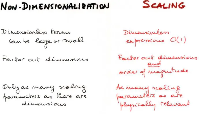
All terms in an equation must have the same dimensions. Without this, changes in units would change the ratio between terms, which is physically impossible. In undergraduate classes (usually in fluid mechanics and in heat transfer), factoring out the dimensions is performed so as to obtain useful dimensionless numbers.
4.3. DIMENSIONLESS EQUATIONS AND SCALING ANALYSIS 111
In scaling analysis, we go one step further. We attempt to use the phys-ically different length scales, say, for each term, so the scales can be vastly different in different directions. Similarly, the velocity components may scale differently, and this should be reflected when factoring out their magnitude. This leads to a proliferation of dimensionless numbers: for example, in a boundary layer, one can define a Reynolds number based on distance from the leading edge, on boundary layer thickness, on momentum thickness, etc. In complex flows such as atmospheric motion, the correct insight may depend on the scaling choices.
Consider a term such as∂yu. In dimensional analysis, one selects a length scale L and a velocity scale U, and factor out the dimensions
∂yu= U
L∂y∗u
∗ (4.7)
Eventually dividing by U
L yields the dimensionless form of the corresponding
equation. In scaling analysis, the perspective is to get a finite difference estimate for the partial derivative: U and L would be such that
∂yu∼ U
L (4.8)
With dimensions as an underlying requirement, the emphasis shifts to having the correct order of magnitude, with the dimensionless partial derivative being replaced by a number roughly comparable to 1 (it could be 3 or 0.2, but not 100). Thus, instead of obtaining an exact dimensionless partial-differential equation, one gets an approximate algebraic equation.
Take the Navier-Stokes equations
∂tui+uj∂jui=−1
ρ∂ip+ν∂ 2
jjui (4.9)
and assume for the time being that the same scaling U and L applies in all directions. Then the nonlinear term scales as
uj∂jui ∼ U
2
L (4.10)
and the viscous term as
ν∂2
jjui ∼ν U
Let us now assume that the flow is such that the convective (nonlinear) term is important; we take is as the yardstick against which the other terms will be evaluated. Then, we have
L U2∂tui+ 1 ∼ − L ρU2∂ip+ ν U L (4.12)
Note that the equality is replaced by an order-of-magnitude estimate. Now, unless there is a separate mechanism (forcing) to impose a distinct time-scale, the time-derivative term can at most be of order 1 (if larger, it makes the convective term negligible, contrary to our assumptions!). Therefore
L
U2∂tui <∼1 (4.13)
which is consistent with a time scale of orderL/U. Similarly for the pressure term, assuming no distinct length scales gives
p∼ρU2
(4.14) as the order of magnitude for pressure variations over distances of orderL.
In this scenario, the orders of magnitude are: less than or comparable to 1 for evolution occuring over times not shorter thanL/U; order 1 for the convective term; order 1 for pressure; and orderν/U L for the viscous term.
Watch out, use the correct scales!
4.4
Rational approximations
Thus, in scaling analyis, the dimensionless parameters are estimates of the relative orders of magnitude of the various terms in an equation, provided the correct parameters have been used. We saw, above, that this can provide orders of magnitude for some parameters so the corresponding terms are comparable to the leading term: time scale and pressure in the previous example. But in other instances, all terms are known (e.g. the viscous term), and their order of magnitude is of critical interest.
In the NS example, the convective term was taken, somewhat arbitrarily, as reference, and is of order 1. If the Reynolds number is large under the correct scaling, this indicates that the viscous term isrelatively small: this is a rational basis for dropping the viscous term (even though large Reynolds
4.4. RATIONAL APPROXIMATIONS 113
number is not the same thing as inviscid: more on this below). Then the equations of motion can be simplified as
∂tui+uj∂jui =−1
ρ∂ip (4.15)
and we have basis for using Euler’s equation, instead of Navier-Stokes. We will study this case in Ch. 5
Conversely, the scaling might indicate that the Reynolds number is very small, in which case the viscous term is much larger than the convective term. The standard assumption of using the convective derivative as references is invalidated: we need to go back to the first step, and instead of Eq.(4.12), we get L2 U ν∂tui+ U L ν ∼ − L2 µU∂ip+ 1 (4.16)
The most obvious is that the convective term can be dropped, yielding Stokes’ equation
∂tui =−1
ρ∂ip+ν∂ 2
jjui (4.17)
to be studied in Ch. 6. A second consequence, less obvious at first, is that the natural time scales and pressure scales are different from the large-Re case. Think about this! The pressure now scales with µU/L (i.e. with a viscous stress), and the time scale is given by L2
/ν.
The same rationale provides useful simplifications in other situations. Unsteady forcing may be treated as quasi-static or as an instantaneous im-pulse, depending on how the time constants match up; the earth’s rotation may dominate the dynamics (large scale atmospheric motion) or be neglected (bathtub vortex); etc. We will touch on these topics in later chapters. But one case needs special consideration, and is so important that a separate subsection seems indicated for emphasis.
4.4.1
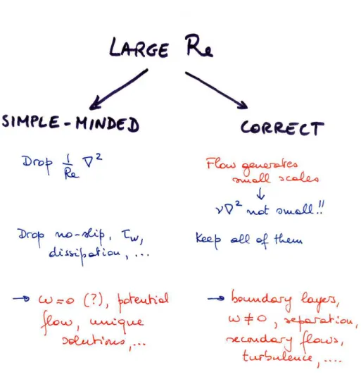
Large Re
What is different about the viscous term is that it contains the highest deriva-tive in the equation. As a general property of such equations, externally imposed scales (Labove) are not sufficient to describe the physics, since the viscous term carries the ability to enforce the no-slip condition.
This quandary is at the core of D’Alembert’s paradox (see Ch. 5), which divided the fluid mechanics community for the better part of the nineteenth
4.5. ADVANCED TOPICS AND IDEAS FOR FURTHER READING 115
century: the potential flow (aerodynamics, etc.) community, willing to over-look zero drag as long as everything else was calculated efficiently, and the hydraulics community, for whom empirical facts won over neat mathematics. Prandtl resolved the conundrum with his idea of the boundary layer: poten-tial flow applies outside this layer, vorticity effects dominate inside. From the viewpoint of scaling, the problem generates its own internal scale (the boundary layer thickness), such that the corresponding Reynolds number is not large, and the highest derivative is no longer negligible! This falls un-der the general heading of singular perturbations (for the mathematically inclined), but the familiar example of the boundary layer (Ch. 8) contains many of the right elements.
4.5
Advanced topics and ideas for further
read-ing
Many examples of scaling analysis appear in turbulence theory and in convec-tive heat transfer. After dimensional analysis, where the dynamical equations are not even used, and control volume analysis, where we integrate over many details, scaling analysis is arguably the simplest way to learn from partial differential equations.
In the limit of very large Re, energy dissipation does not behave as simply as the formula (Ch. 3) suggests: as the flow becomes turbulent, the scaling of the rate-of-strain no longer follows the externally imposed length or velocity scales, but instead follows the scaling of the turbulence. Thus, the dissipation rate becomes independent of viscosity! See your turbulence course for more on this surprising result, which shows again that Re → ∞ is not a simple limit. Another instance is the boundary layer (see Ch. 8).
Problems
Some of these problems have been adapted from Tritton’s, from Fox and McDonald’s and from Munson and Okiishi’s books.
1. Consider the vortex shedding behind a cylinder. The shedding fre-quency f is assumed to be a function of diameter d, flow speed V, and fluid properties ρ and µ. Determine the form of the relation between dimensionless frequency and velocity.
4.5. ADVANCED TOPICS AND IDEAS FOR FURTHER READING 117
2. The size d of droplets produced by a liquid spray nozzle is thought to depend on the nozzle diameter D, jet velocity U, and the properties of the liquid ρ (density), µ(dynamic viscosity) andσ (surface tension, which is an energy per unit area). Construct the dimensionless products to show the dependence of drop size on surface tension and speed; modify the result to express the dependence of drop size on viscosity and surface tension.
3. The lift force on a Frisbee is thought to depend on its rotation speed, translation speed and diameter as well as air density and viscosity. Determine the dimensionless parameters in the relation showing lift as a function of the two speeds. Then modify the relation to express the dependence of lift on diameter.
4. The shaft power input P into a pump depends on the volume flow rate Q, the pressure rise dp, the rotational speed N, the fluid density
ρ, the impeller diameter D, and the fluid viscosity µ. Express the dimensionless dependence of power on flow rate, pressure rise and other applicable parameters; discuss alternatives. What happens to your result if you learn eventually that P =Q dp?
5. The power P required to drive a fan depends on the fluid density ρ, on the fan diameter D and angular speed ω, and on the volume flow rate
Q. Derive the dimensionless relation showing how power depends on diameter. Reformulate the result to show how power depends on flow rate.
6. Incompressible steady flow in a magnetic field combines the equations of motion (with addition of the Lorentz force) ∇ · u = 0, u· ∇u = −1ρ∇p+ 1
ρµ(∇×B)×B+ν∇ 2
uwith the equations for magnetic induction ∇ ·B = 0,u· ∇B =B· ∇u+ 1
σµ∇ 2
B. (here,µis magnetic permeability and σ is electrical conductivity). What are the similarity parameters? Discuss their physical meaning. (Problem 21 p.474 from Tritton.) 7. Dimensional analysis for pulsatile flow in a pipe: discuss the additional
parameters and carry out the analysis.
8. Dimensional analysis of laminar flow in a helical pipe: discuss the ad-ditional parameters and find the dimensionless products.
9. Discuss the use of the sphere drag data in relation to improved fuel economy at lower highway speeds.
10. Scaling analysis of Bernoulli’s equation, taking U and L as scaling pa-rameters. Under what conditions can we ignore gravity? Read up on the corresponding dimensionless number and give a half-page summary. 11. Use scaling analysis to find the time scale of relaxation for 1-D thermal
conduction∂tT =α∂2 jjT