DEVELOPMENT AND APPLICATION OF MICROFLUIDIC CAPILLARY
ELECTROPHORESIS-ELECTROSPRAY IONIZATION DEVICES FOR THE ANALYSIS OF BIOLOGICAL SAMPLES
William A. Black
A dissertation submitted to the faculty at the University of North Carolina at Chapel Hill in partial fulfillment of the requirements for the degree of Doctor of Philosophy in the Department
of Chemistry.
Chapel Hill 2015
Approved by:
J. Michael Ramsey
James W. Jorgenson
Matthew R. Lockett
Mark Tommerdahl
ABSTRACT
William A. Black: Development and Application of Microfluidic Capillary Electrophoresis-Electrospray Ionization Devices for the Analysis of Biological Samples
(Under the direction of J.M. Ramsey)
ACKNOWLEDGEMENTS
First and foremost, I would like to thank my advisor, Dr. J. Michael Ramsey. I am extremely thankful for the opportunity to work in your lab, and all that I have learned and gained from the experience. I am especially grateful for the confidence you have displayed in me, and for reminding me to always strive for excellence. I am also very appreciative of the freedom you granted me during my time at UNC to explore my interests, both inside and outside of the laboratory.
I also indebted to the past and current members of the Ramsey lab for a vast amount of knowledge, support, and help throughout the last five years. J.P. Alarie, Scott Mellors, Nick Batz, Erin Redman, Hamp Henley, Mac Gilliland, Esme Candish, and Rob Musser deserve special mention for their contributions to my learning and success. I would also like to thank the lab as a whole for instilling and sustaining a culture of collaboration and
collegiality, which made working here much more fun.
I would also like to thank my roommates, Marie-Angela, Isaac, and Rocket for their good humor and support while I chased my degree. We had a lot of good times at 34 Clover Dr. It’s the end of an era, but another one has just begun!
My family also deserves much of the credit for supporting me and assisting me throughout this process and throughout my life. My parents and my sister Christina have been an amazing source of encouragement and help, and I am deeply grateful. I am thankful for the encouragement to pursue my passions and for always being there throughout the ups and downs. I certainly would not be where I am today without my family.
TABLE OF CONTENTS
LIST OF TABLES……….xv
LIST OF FIGURES………xvi
LIST OF ABBREVIATIONS……….…xxi
LIST OF SYMBOLS………xxiii
CHAPTER 1: INTRODUCTION………..1
1.1 Importance of Biological Analysis………..1
1.2 Electrophoresis………....2
1.3 Capillary Electrophoresis………3
1.4 Capillary Electrophoresis-Mass Spectrometry………6
1.5 Microfluidic Devices………...8
1.6 Work Described in This Thesis………..11
1.7 References………..13
CHAPTER 2: A HYBRID CAPILLARY/MICROFLUIDIC SYSTEM FOR COMPREHENSIVE ONLINE LIQUID CHROMATOGRAPHY-CAPILLARY ELECTROPHORESIS-ELECTROSPRAY IONIZATION-MASS SPECTROMETRY…...17
2.2 Experimental………..22
2.2.1 Reagents and Materials………...22
2.2.2 Microchip Design and Fabrication………..23
2.2.3 Surface Modifications……….25
2.2.4 Liquid Chromatography………..26
2.2.5 Microchip Operation………...27
2.2.6 Mass Spectrometry………..28
2.2.7 Data Processing………...28
2.2.8 High Acquisition Rate LC-CE-ESI……….30
2.3 Results and Discussion………..32
2.3.1 Evaluation of System Performance……….32
2.3.2 N-Linked Glycosylation Analysis of a Monoclonal Antibody………...37
2.3.3 Increased Acquisition Rate LC-CE……….42
2.4 Conclusions………47
2.5 References………..49
3.1 Introduction………52
3.2 Experimental………..57
3.2.1 Reagents and Materials………...57
3.2.2 Microchip Design and Fabrication………..57
3.2.3 Microchip Surface Coating……….59
3.2.4 Hydrogen Deuterium Exchange Sample Preparation and Workflow….60 3.2.5 Microchip Operation………...60
3.2.6 LC-MS Operation………...62
3.2.7 Complex Mixture Sample Preparation and Separation………...63
3.2.8 Data Processing………...64
3.3 Results and Discussion………...64
3.3.1 CE-ESI Separation Performance……….64
3.3.2 MS Performance……….68
3.3.3 Sequence Coverage and Limitations………...71
3.3.4 Deuterium Recovery………...74
3.3.5 Complex Mixture Analysis……….77
3.5 References………..80
CHAPTER 4: LOW TEMPERATURE MICROCHIP CAPILLARY-ELECTROPHORESIS ELECTROSPRAY-IONIZATION………..83
4.1 Introduction………....83
4.2 Experimental………..86
4.2.1 Reagents and Materials………...86
4.2.2 Microchip Design, Fabrication, and Surface Coating……….86
4.2.3 Peltier Cooling Device………88
4.2.4 Microchip CE-ESI Operation……….89
4.2.5 Temperature Controlled Separations………..91
4.2.6 Stopped Flow………..91
4.2.7 Microchip CE-ESI Infusion………92
4.2.8 Hydrogen Deuterium Back Exchange………92
4.2.9 Data Processing………...93
4.3 Results and Discussion………..94
4.3.1 CE-ESI Separation Performance……….94
4.3.2 ESI Performance………...101
4.4 Conclusions………..109
4.5 References………111
CHAPTER 5: INTEGRATING SOLID PHASE EXTRACTION AND TRANSIENT ISOTACHOPHORESIS WITH MICROCHIP CAPILLARY ELECTROPHORESIS-ELECTROSPRAY IONIZATION………113
5.1 Introduction……….…….113
5.2 Experimental………117
5.2.1 Reagents and Materials……….117
5.2.2 Microchip Design, Fabrication, and Surface Coating………...117
5.2.3 Microchip CE-ESI Operation……….……..118
5.2.4 Microchip SPE-CE-ESI Operation………...119
5.2.5 Separation of a Four Peptide Mix……….120
5.2.6 Electrokinetic and Hydrodynamic Injection Comparison……….120
5.2.7 Sample Carryover……….121
5.2.8 Protein Digest Separations………122
5.2.9 Data Processing……….122
5.3 Results and Discussion………123
5.3.1 Separation and Pre-concentration Performance………123
5.3.3 Complex Mixture Separations………..138
5.4 Conclusions………..142
5.5 References………....143
CHAPTER 6: CONCLUSIONS AND FUTURE WORK……….146
6.1 Multidimensional Separations……….146
6.1.1 Summary………...146
6.1.2 Increased MS Acquisition Rate………147
6.1.3 Alternate Chromatography Modes………150
6.2 Microchip CE-ESI for Hydrogen/Deuterium Exchange………..150
6.2.1 Summary………...150
6.2.2 Coupling with Improved Mass Spectrometer………...151
6.2.3 Low Temperature Microchip CE-ESI………...151
6.2.4 Integrated Sample Processing………...152
6.3 Low Temperature Microchip CE-ESI………..153
6.3.1 Summary………...………153
6.3.2 Optimization of ESI Performance……….154
6.3.4 Condensation……….155
6.4 Integrated Sample Processing………..157
6.4.1 Summary………...157
6.4.2 Alternate Stationary Phases………..158
6.4.3 Increasing Bed Capacity………...158
6.4.4 Sample Cleanup Optimization………..162
LIST OF TABLES
Table 2.1. N-linked glycopeptides observed by LC-CE-MS analysis of the IgG2 tryptic digest………39
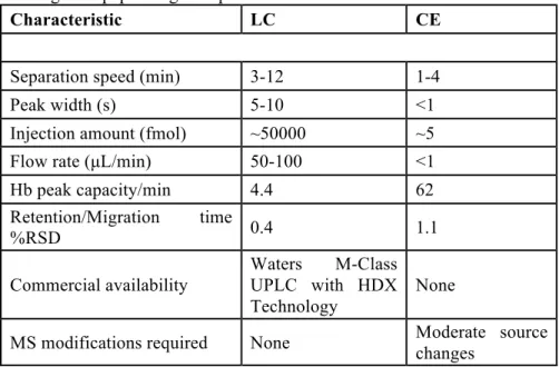
Table 3.1. Comparison of CE and LC figures of merit for bovine hemoglobin pepsin digest separation……….68
Table 4.1. Calculated Δ values of the 4 peptides at 2 different temperatures……….98
Table 4.2. Dm and Dapp values (x 10-6 cm2/sec) for 4 peptides at 2 different temperatures…98
Table 4.3. Calculated relative deuterium uptake values for peptides at various
conditions...108
LIST OF FIGURES
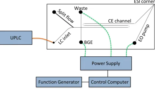
Figure 2.1. Schematic of the hybrid capillary LC-microchip CE-ESI experimental setup with a 9 cm long separation channel. The orange line represents a transfer capillary connecting the LC column to the microfluidic device. The dashed green lines represent electrical connections between the high voltage power supply and the microfluidic reservoirs. The device was positioned with the ESI corner approximately 5 mm from the mass
spectrometer inlet. Channel dimensions are given in the experimental section……..………24
Figure 2.2. Structures of common N-linked glycans examined in this manuscript…………29
Figure 2.3. Schematic of the hybrid capillary LC-microchip CE-ESI experimental setup with a 4.3 cm long separation channel. The orange line represents a transfer capillary connecting the LC column to the microfluidic device. The dashed red lines represent electrical connections between the high voltage power supply and the microfluidic
reservoirs………31
Figure 2.4. LC-MS chromatogram (A), and LC-CE-MS chromato-electropherogram (B/C) for the analysis of a 5-protein tryptic digest mixture. All LC conditions and MS acquisition settings were identical for these two runs. The bottom plot (C) is an expanded view of a segment of the data shown in B. The dashed lines indicate when CE injections were
performed, with labels to indicate the injection number………32
Figure 2.5. Image plot for the LC-CE-MS separation of a 5-protein tryptic digest mixture. This plot was generated from the same data shown in figure 2.3B……….34
Figure 2.6. Extracted ion plots for the LC-MS (red) and LC-CE-MS (black) separations of the 5-protein tryptic digest. The LC-MS trace was shifted by +0.45 min to better align the peaks for better visual comparison; and the LC-CE-MS trace was shifted down by 20 counts to align the baselines………35
Figure 2.8. Image plot for the LC-CE-MS separation of a digested IgG2 containing two N-linked glycosylation sites. The circled spots contained all of the observed N-N-linked
glycopeptides. The spot labeled A0 contained all of the glyopeptides from the Fc domain site. Spots B0, B1, and B2 contained the glycopeptides from the Fab domain site containing 0, 1, and 2 sialic acid residues, respectively. The positions of corresponding unglycosylated
peptides from each site are indicated with asterisks (*)………..38
Figure 2.9. Multidimensional image plot showing the LC-CE-MS separation of a 4-protein tryptic digest mixture. A total peak capacity of 320 was observed……….44
Figure 2.10. Representative image plots illustrating the data handing capabilities of Driftscope software. A – Chromato-electropherogram mage plot showing the location of a specific m/z value (689 m.z). B – Plot illustrating the LC peak shape and data points per peak of the selected component. C – Plot illustrating the CE peak shape and data points per peak of the selected component. D – Mass spectrum showing the spectral data of the selected analyte………...47
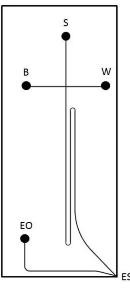
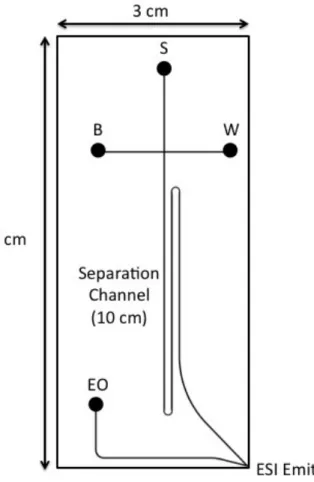
Figure 3.1. Schematic of CE-ESI Microchip. The reservoir labels correspond to sample (S), background electrolyte (B), sample waste (W), and electroosmotic pump (EO). The
separation channel measures 10 cm long. The dimensions of the chip are approximately 3 cm wide by 6 cm long………58
Figure 3.2. CE-MS (top) versus LC-MS (bottom) of the same bovine hemoglobin pepsin digest. CE-ESI was performed at room temperature while LC-MS was performed at 0 °C………..66
Figure 3.3. Representative peak profiles from bovine hemoglobin pepsin digest showing data points across peak for CE (top) and LC (bottom)………....69
Figure 3.4. Measured deuterium level comparison for six representative peptic peptides from bovine hemoglobin. Error bars, representing standard deviation of duplicate measurements, are present but in most cases too small to see………..75
Figure 4.1. Microchip CE-ESI schematic. Reservoirs correspond to sample (S), background electrolyte (B), waste (W), and electroosmotic pump (EO). ESI denotes the electrospray emitter. Dashed line corresponds to the border of the Peltier thermoelectric device………..87
Figure 4.2. Instrumental setup for the Peltier cooling device. The dotted black line corresponds to the relationship between the microchip and the Peltier. ESI and MS
correspond to electrospray emitter and mass spectrometer, respectively. Drawing not to scale; however, the relationship in size between the chip, Peltier, and water block is accurate…....88
Figure 4.3. Microchip CE-ESI electropherograms of a 4-peptide mix at different temperatures (30 °C to 0 °C) and constant applied voltage, yielding a field strength of 1050 V/cm. Electropherograms offset for visualization………...95
Figure 4.4. Plot of efficiency versus temperature for the 4 peptides. Error bars represent standard error (n = 3 to 6)……….………...97
Figure 4.5. Electropherograms of a 4-peptide mix at 25 °C and 790 V/cm electric field strength and at 0 °C and 1475 V/cm electric field strength………..……….102
Figure 4.6. Infusion data of 500 nM fluorescein. Error bars represent standard error (n=6). The top plot and the bottom plot share the same Y-axis, but the X-axis is plotted as either temperature (top) or volumetric flowrate (bottom)………..………..104
Figure 4.7. Calculated peak area for 4-peptide mix at various temperatures. The field
strength was 1055 V/cm……….105
Figure 4.8. Mass spectra of 2+ charge state of Angiotensin II. A – undeuterated sample at 25 °C, 875 V/cm. B – deuterated sample at 25 °C, 875 V/cm. C – deuterated sample at 0 °C, 875 V/cm. D – deuterated sample at 0 °C, 1475 V/cm. R.D.U. corresponds to relative
Figure 5.1. Schematic and experimental set up of the SPE-CE-ESI microchip. The separation channel (S) is 23 cm long, and all channels are 10 µm deep. Applied voltage, pressure, and vacuum are controlled by a computer with a Labview program. The dimensions of the SPE bed are not to scale, but enlarged to show location………...……118
Figure 5.2. Electropherograms of 4-peptide mix. Top – CE-ESI of 5 µM sample. Middle – SPE-CE-ESI of 50 nM sample. Bottom – SPE-tITP-CE-ESI of 50 nM sample…….…..…124
Figure 5.3. Electropherograms of a four peptide mix comparing electrokinetic injection (top) versus hydrodynamic injection (bottom)………...127
Figure 5.4. Peak area comparison of microchip CE-ESI of four peptides for electrokinetic and hydrodynamic injections………...128
Figure 5.5. SPE-tITP-CE-ESI electropherograms of increasing concentrations of a 4-peptide mix……….134
Figure 5.6. Plots illustrating peak area, width, and height for SPE-tITP-CE-ESI analysis of bradykinin, thymopentin, and an unidentified trace component labeled peptide A. The concentration of the peptide mix loaded ranged from 1 nM to 10 µM. Sample concentration reflects the concentration of the 4 peptides in the mixture (thymopentin, bradykinin,
angiotensin II, and met-enkephalin) and does not represent the concentration of the trace components A and B………..135
Figure 5.7. Peak area, peak width, and peak height for angiotensin II, met-enkephalin, and unidentified peptide B (Figure 5.3). The concentration of the sample loaded ranged from 1 nM to 10 µM………..137
Figure 5.8. Electropherograms of Phosphorylase B tryptic digests separated using CE-ESI (5 µM) and SPE-tITP-CE-ESI (50 nM). The CE-ESI electropherogram has been offset for visualization. The inset shows an expanded view of the CE-ESI electropherogram……….140
Figure 5.9. Electropherogram of SPE-tITP-CE-ESI separation of 0.5 mg/mL E. Coli
Figure 6.1 Base peak index electropherogram for the high-speed CE-ESI-MS separation of a mixture containing fluorescein, methionine enkephalin, angiotensin II, bradykinin and thymopentin (listed from shortest to longest migration time). Data were obtained using a 3 cm device at an electric field strength of A) 500 V/cm and B) 1,500 V/cm. Figures and data courtesy of Dr. Nick Batz………..149
Figure 6.2. Photograph depicting a humidity controlled system for performing low temperature microchip CE ESI. The white square corresponds to the Peltier device. Cable guides on the top of the enclosure provide access vias for applied voltage leads………….156
LIST OF ABBREVIATIONS
2D Two Dimensional
APDIPES Aminopropyldiisopropylethoxysilane APTES Aminopropyltriethoxysilane
BGE Background Electrolyte BPI Base Peak Ion Count
CE Capillary Zone Electrophoresis CVD Chemical Vapor Deposition
EO Electroosmotic
EOF Electroosmotic Flow ESI Electrospray Ionization
GC Gas Chromatography
GMO Genetically Modified Organisms
Hb Hemoglobin
HILIC Hydrophilic Interaction Chromatography HPLC High Performance Liquid Chromatography HX MS Hydrogen Exchange Mass Spectrometry IEF Isoelectric Focusing
IgG2 Immunoglobulin G2 IMS Ion Mobility Spectroscopy
KOH/IPA Potassium Hydroxide in 2-propanol LC Liquid Chromatography
LE Leading Electrolyte
MALDI Matrix Assisted Laser Desorption/Ionization
min Minutes
MS Mass Spectrometry
PAGE Polyacrylamide Gel Electrophoresis PEG Polyethylene Glycol
PLGS ProteinLynx Global Server ppm Parts per Million
qTOF Quadrupole - Time of Flight RTD Resistance Temperature Detector RSD Relative Standard Deviation
s Seconds
S/N signal to noise ratio SPE Solid Phase Extraction TE Trailing Electrolyte
tITP Transient Isotachophoresis
TRIS tris(hydroxymethyl)aminomethane
UPLC Ultra Performance Liquid Chromatography
UV Ultraviolet
LIST OF SYMBOLS v Electrophoretic Velocity
µ Electrophoretic Mobility
E Electric Field
q Charge
η Viscosity
r Hydrodynamic Radius
N Theoretical Plates
L Capillary Length
V Applied Voltage
D Diffusion Coefficient
T Temperature
t Time
Da Dalton
nc Peak Capacity
X Separation Window
σ Standard Deviation
Hz Hertz
k Boltzmann’s constant
°C Degrees Celsius
I Spectral Intensity σ2 Spatial Variance
m Centroid Mass
m0% Undeuterated Centroid Mass Dapp Apparent Diffusion Coefficient Dm Measured Diffusion Coefficient
CHAPTER 1: INTRODUCTION
1.1 Importance of Biological Analysis
To facilitate a deeper understanding of these biological processes, it’s necessary to comprehend the mechanisms and pathways and their constituents on a molecular level. In order to perform these investigations, analytical techniques that can probe these molecules, such as proteins, peptides, carbohydrates, small molecules, and nucleic acids are needed. Methods to characterize these molecules and their interactions have been the focus of the scientific community for decades. Countless techniques and instruments have been developed and great strides have been made in numerous fields since the mid 19th century. However, further improvements are necessary to realize the lofty goal of fully understanding biological systems and translating that knowledge to the macro environment. Advancements in the technology used to study biological processes will likely result in impactful gains to numerous biomedical, agricultural, and industrial applications and yield tangible benefits to society.
1.2 Electrophoresis
Since the initial descriptions of blood serum protein separations in 1937 by Tiselius, 5-9 electrophoresis has been an invaluable tool for the analysis of biological samples.10,11
Electrophoresis is defined as the movement of a charged species in a fluid or gel under the influence of an electric field. Equation 1 describes the electrophoretic velocity (v) of an analyte, where µ corresponds to the electrophoretic mobility of that analyte and E corresponds to the applied electric field.12
v
=
µE
(1)
µ
=
q
6πηr
(2)As illustrated by Equation 2, electrophoresis separates analytes primarily based on the molecule’s charge-to-size ratio. For analytes that have the same charge-to-size ratio, such as DNA, the addition of a sieving medium, such as cross-linked polyacrylamide, results in a size based separation.10 In the nearly 80 years since the seminal publications, many different forms of electrophoresis have been applied to a wide variety of applications, including but not limited to polyacrylamide gel electrophoresis (PAGE),13,14 agarose gel electrophoresis,15,16 free flow electrophoresis,17,18 isoelectric focusing (IEF),19,20 and isotachophoresis.21,22 Two dimensional denaturing PAGE (2D PAGE) in particular, the coupling of IEF in the first dimension and PAGE in the second dimension, has become an extremely powerful technique for the analysis of intact proteins. To date, more than 10,000 protein spots can be resolved by a single gel, which are typically 15 x 20 cm in size.10 However, the technique is not without disadvantages. Despite the impressive resolving power and decade of routine use, 2D PAGE is time consuming, labor intensive, only semi-quantitative, has limited detection methods, and has historically not performed well with low abundance or hydrophobic proteins.14
1.3 Capillary Electrophoresis
application, detection, quantification, and automated operation.23 Stabilizing media were required to suppress the convective flow that arose from the application of voltage to the electrophoretic system. The passage of an electric field yields the generation of heat. As heat is generated across the entire electrophoretic system but only removed at the edges, a radial heat gradient forms, resulting in the unwanted spreading of analyte bands.23,24 The heat gradient causes analyte zone broadening in multiple ways. First, the higher temperature fluid in the center of the system will be less dense than the cooler fluid at the edges, resulting in convective current. Second, the higher temperature fluid will also be less viscous, resulting in increased analyte mobility.23,24 The use of stabilizing media reduced the convective flow observed but does not address the generation of the heat gradient. Furthermore, the stabilizing media also added to broadening of the analyte zones through eddy migration.23,24 Therefore, the removal of the stabilizing gel from the electrophoretic system would have many advantages, including easier adoption of an instrumental method, which could automate many functions, as well as reduced zone broadening, increasing separation performance.
generation of the radial thermal gradient. While thermal gradients in the capillary cannot be eliminated entirely, the narrow tube diameter helps to reduce the influence of the thermal gradient on zone broadening through ‘averaging’ of the analytes’ radial position throughout the separation. A thermal gradient only imparts zone broadening if molecules spend an extended period of time in either the hot or cool radial region of the capillary. By decreasing the radius of the capillary, analytes can diffuse across the entire radial dimension of the capillary on the time scale of the separation, reducing the effect of the temperature gradient broadening.23,24 The culmination of these effects to reduce broadening result in a technique capable of producing very high separation efficiencies. Equation 324 illustrates the number of theoretical plates (N) for a CE separation, where V is the applied voltage, D is the diffusion coefficient, and µ is the electrophoretic mobility. Equation 424 illustrates the required migration time (t) for an analyte, where L is the capillary length.
N
=
µV
2D
(3)
t
=
L
2µV
(4)wide analysis scope as CE has been applied to nearly every biological sample imaginable including nucleic acids,27,28 amino acids,29,30 peptides,31,32 proteins,33,34 organelles,35,36 viruses,37,38 and whole cells.39,40 Most of the early work focused on CE analysis utilized optical detection methods, such as UV absorbance of fluorescence detection. While UV absorbance detection is widely applicable to many different analytes, the sensitivity of the method is a concern. Fluorescence detection is quite sensitive, but only certain analyte are naturally fluorescent, and labeling the analytes with a fluorescent tag can have a negative effect on the analysis of the analytes of interest. Furthermore, optical detection methods do not provide any mass or structural identification data. As the scope of analysis grew for many applications and sample complexity increased, detection methods that provided additional structural identification, sensitivity, and universal application were desired.41
1.4 Capillary Electrophoresis– Mass Spectrometry
Although CE and ESI share common properties, such as employing simple direct current circuits, strategies for the coupling of the two techniques must address several fundamental issues, including consolidation of the CE and ESI circuits, stable electric contact at the CE outlet electrode, proper emitter geometry for supporting stable ESI, and suitable electrolyte for separation and ESI.53 To date, the most common method for coupling CE and ESI is a sheath flow configuration that utilizes a coaxial arrangement of three concentric tubes. The inner tube is the separation column, followed by metal tubing for sheath liquid delivery, and finally outer tubing for the application nebulizer gas. The sheath liquid establishes electrical contact between the metal sheath flow tube, which functions as the CE outlet electrode and the electrospray emitter.53 Unfortunately, this arrangement has two significant disadvantages. First, the high flow rate of sheath liquid dilutes the CE effluent, resulting in decreased sensitivity. Second, the application of a nebulizing gas causes a suction effect at the outlet of the CE capillary, introducing parabolic flow and decreasing the separation efficiency.53 In 2007, Moini introduced a porous tip emitter that performed CE-MS without the use of sheath flow.54 The porous sprayer tip is made by etching a segment of the capillary outlet, which permits the transport of small ions across the porous wall. The porous tip is then inserted into a metal sheath filled with BGE. A second capillary is inserted into the sheath, and an applied voltage forms the electric connection at the outlet of the CE separation capillary.54 This approach reduces the dilution effect of using a sheath flow, and has been applied to a number of different analytes including small molecules, peptides, and proteins.55-57
Another strategy for coupling CE with ESI is to use a microfluidic device. Microchips, or lab-on-a-chip technologies, were developed in the early 1990’s and popularized by Ramsey and co workers.58-62 Microfluidic devices utilize the advancements in microfabrication techniques available for the microelectronics industry to generate tools for chemical sensing and analysis.60 In 1994, Jacobson et al. demonstrated a microchip monolithically etched in glass for performing CE with optical detection.60 Microfluidic devices have many advantages when compared with bench top instruments, including high speed,58,63 precise control of small sample volumes with no dead volume,64,65 low reagent and sample volume requirements,65,66 small physical footprint,60-62,64 the ability to integrate multiple components onto a single device,64,67,68 and the ability to automate the necessary steps of chemical analysis.67,69,70 Furthermore, the ability to automate many of the analysis steps leads to improvements in reproducibility, and can result in enhanced performance.65,71 Since the initial descriptions in the early 1990’s, microfluidic devices have been applied to dozens of different applications, and their potential for improving the analysis of biological samples has been thoroughly investigated.
pump channel resulted in differences to the EOF, which generated pressure driven flow to force fluid out of the ESI emitter. The EO pump channel also served to complete the CE circuit and control the voltage applied to the ESI emitter.41 The design by Mellors et al. combines the benefits circumventing sheath flow for CE-MS as well as the numerous advantages of microfluidic devices.
Since the initial description by Mellors et al., the integrated CE-ESI microchip has been demonstrated to be a powerful tool for the analysis of biological samples. In 2010, Mellors et al. described a method for using the device to analyze the contents of cells lysed on chip.65 Chambers et al. demonstrated the coupling of microchip CE-ESI with a monolithically integrated LC column for a multi-dimensional separation of complex peptide mixtures.64 Batz et al. described a novel method for surface coatings in microfluidic devices.71 The improved surface coatings, as well as the reduction of other band broadening sources by using microchips such as injection and detector broadening,60 resulted in near diffusion limited separations.71 Redman et al. described a microfluidic CE-ESI method for the resolution of intact monoclonal antibody variants.72
1.6 Work Described In This Thesis
hydrogen/deuterium exchange mass spectrometry (HX MS). The separation of a bovine hemoglobin pepsin digest was utilized to characterize the compatibility of an HX MS protocol with microchip CE-MS as well as quantifying the separation and mass spectrometry performance. A deuterium labeling experiment was performed to compare the deuterium retention of a microchip CE-MS method relative to an UPLC-MS method. A 270 kDa protein pepsin digest was also used to characterize the performance of the microchip CE-MS method for complex mixtures of large protein systems.
1.7 REFERENCES (1)!Oliver,!M.!J.!Missouri'medicine!2014,!111,!4928507.!
(2)!Monastra,!G.;!Rossi,!L.!Rivista'di'biologia!2003,!96,!3638384.! (3)!American!Cancer!Society.;!The!Society:!Atlanta,!GA,!2014,!p!v.!
(4)! Yabroff,! K.! R.;! Lund,! J.;! Kepka,! D.;! Mariotto,! A.!Cancer' Epidemiol' Biomarkers' Prev' 2011,!20,!200682014.! ! (5)!Tiselius,!A.!J'Exp'Med!1937,!65,!6418646.! (6)!Tiselius,!A.!Skand'Arch'Physiol!1937,!77,!84885.! (7)!Tiselius,!A.!Biochem'J!1937,!31,!3138317.! (8)!Tiselius,!A.!T'Faraday'Soc!1937,!33,!052480530.! (9)!Tiselius,!A.!Biochem'J!1937,!31,!146481477.!
(10)! Kleparnik,! K.;! Bocek,! P.!BioEssays' :' news' and' reviews' in' molecular,' cellular' and' developmental'biology!2010,!32,!2188226.! ! (11)!Subirats,!X.;!Blaas,!D.;!Kenndler,!E.!Electrophoresis!2011,!32,!157981590.! (12)!Landers,!J.!P.!Handbook'of'capillary'electrophoresis,!2nd!ed.;!CRC!Press:!Boca!Raton,! 1997,!p!894!p.! ! (13)!Chrambach,!A.;!Rodbard,!D.!Science!1971,!172,!4408451.!
(21)!Mala,!Z.;!Gebauer,!P.;!Bocek,!P.!Electrophoresis!2013,!34,!19828.! (22)!Smejkal,!P.;!Bottenus,!D.;!Breadmore,!M.!C.;!Guijt,!R.!M.;!Ivory,!C.!F.;!Foret,!F.;!Macka,! M.!Electrophoresis!2013,!34,!149381509.! ! (23)!Jorgenson,!J.!W.;!Lukacs,!K.!D.!Science!1983,!222,!2668272.! (24)!Jorgenson,!J.!W.;!Lukacs,!K.!D.!Clin'Chem!1981,!27,!155181553.!
(25)!Mikkers,!F.!E.!P.;!Everaerts,!F.!M.;!Verheggen,!T.!P.!E.!M.!J'Chromatogr!1979,!169,! 11820.! ! (26)!Puig,!P.;!Borrull,!F.;!Calull,!M.;!Aguilar,!C.!Anal'Chim'Acta!2008,!616,!1818.! (27)!Karger,!B.!L.;!Guttman,!A.!Electrophoresis!2009,!30'Suppl'1,!S1968202.! (28)!Nai,!Y.!H.;!Powell,!S.!M.;!Breadmore,!M.!C.!J'Chromatogr'A!2012,!1267,!289.! (29)!Ou,!G.;!Feng,!X.;!Du,!W.;!Liu,!X.;!Liu,!B.!F.!Anal'Bioanal'Chem!2013,!405,!790787918.! (30)!Poinsot,!V.;!Ong8Meang,!V.;!Gavard,!P.;!Couderc,!F.!Electrophoresis!2014,!35,!50868.! (31)!Moore,!A.!W.,!Jr.;!Jorgenson,!J.!W.!Anal'Chem!1995,!67,!346483475.! (32)!Moseley,!M.!A.;!Deterding,!L.!J.;!Tomer,!K.!B.;!Jorgenson,!J.!W.!Anal'Chem!1991,!63,! 1098114.! ! (33)!Haselberg,!R.;!de!Jong,!G.!J.;!Somsen,!G.!W.!Electrophoresis!2011,!32,!66882.! (34)!Haselberg,!R.;!de!Jong,!G.!J.;!Somsen,!G.!W.!Electrophoresis!2013,!34,!998112.!
(35)! Duffy,! C.! F.;! Fuller,! K.! M.;! Malvey,! M.! W.;! O'Kennedy,! R.;! Arriaga,! E.! A.!Anal'Chem! 2002,!74,!1718176.! ! (36)!Duffy,!C.!F.;!Gafoor,!S.;!Richards,!D.!P.;!Admadzadeh,!H.;!O'Kennedy,!R.;!Arriaga,!E.!A.! Anal'Chem!2001,!73,!185581861.! ! (37)!Okun,!V.;!Ronacher,!B.;!Blaas,!D.;!Kenndler,!E.!Anal'Chem!2000,!72,!255382558.! (38)!Okun,!V.!M.;!Ronacher,!B.;!Blaas,!D.;!Kenndler,!E.!Anal'Chem!1999,!71,!202882032.! (39)!Armstrong,!D.!W.;!Schulte,!G.;!Schneiderheinze,!J.!M.;!Westenberg,!D.!J.!Anal'Chem! 1999,!71,!546585469.! !
(60)! Jacobson,! S.! C.;! Hergenroder,! R.;! Koutny,! L.! B.;! Warmack,! R.! J.;! Ramsey,! J.! M.! Analytical'Chemistry!1994,!66,!110781113.! ! (61)!Jacobson,!S.!C.;!Hergenroder,!R.;!Moore,!A.!W.;!Ramsey,!J.!M.!Anal'Chem'1994,!66,! 412784132.! !
(62)! Jacobson,! S.! C.;! Koutny,! L.! B.;! Hergenroder,! R.;! Moore,! A.! W.;! Ramsey,! J.! M.!Anal' Chem!1994,!66,!347283476.!
!
(63)! Jacobson,! S.! C.;! Culbertson,! C.! T.;! Daler,! J.! E.;! Ramsey,! J.! M.!Anal'Chem!1998,!70,! 347683480.!
!
(64)! Chambers,! A.! G.;! Mellors,! J.! S.;! Henley,! W.! H.;! Ramsey,! J.! M.!Anal'Chem!2011,!83,! 8428849.! ! (65)!Mellors,!J.!S.;!Jorabchi,!K.;!Smith,!L.!M.;!Ramsey,!J.!M.!Anal'Chem!2010,!82,!9678973.! (66)!McClain,!M.!A.;!Culbertson,!C.!T.;!Jacobson,!S.!C.;!Allbritton,!N.!L.;!Sims,!C.!E.;!Ramsey,! J.!M.!Anal'Chem!2003,!75,!564685655.! ! (67)!Mellors,!J.!S.;!Black,!W.!A.;!Chambers,!A.!G.;!Starkey,!J.!A.;!Lacher,!N.!A.;!Ramsey,!J.!M.! Anal'Chem!2013,!85,!410084106.! ! (68)!Oblath,!E.!A.;!Henley,!W.!H.;!Alarie,!J.!P.;!Ramsey,!J.!M.!Lab'Chip!2013,!13,!132581332.! (69)!Guetschow,!E.!D.;!Steyer,!D.!J.;!Kennedy,!R.!T.!Anal'Chem!2014,!86,!10373810379.! (70)!Nie,!S.;!Henley,!W.!H.;!Miller,!S.!E.;!Zhang,!H.;!Mayer,!K.!M.;!Dennis,!P.!J.;!Oblath,!E.!A.;! Alarie,!J.!P.;!Wu,!Y.;!Oppenheim,!F.!G.;!Little,!F.!F.;!Uluer,!A.!Z.;!Wang,!P.;!Ramsey,!J.!M.;! Walt,!D.!R.!Lab'Chip!2014,!14,!108781098.! ! (71)!Batz,!N.!G.;!Mellors,!J.!S.;!Alarie,!J.!P.;!Ramsey,!J.!M.!Anal'Chem!2014,!86,!349383500.!
CHAPTER 2: A HYBRID CAPILLARY/MICROFLUIDIC SYSTEM FOR COMPREHENSIVE ONLINE LIQUID CHROMATOGRAPHY-CAPILLARY ELECTROPHORESIS-ELECTROSPRAY IONIZATION-MASS SPECTROMETRY 2.1 Introduction
In recent years, the investigation of biological samples has trended towards the analysis of increasingly complex samples. Bottom up or shotgun proteomics is a salient example, where the entire proteome of a tissue sample, cell, or organism is digested into peptides and subsequently separated and analyzed with mass spectrometry.1,2 PeptideCutter is a software program that predicts potential cleavages sites by protease enzymes. It estimates that the tryspin digest of just a single 70 kDa protein, Bovine Serum Albumin, results in roughly 80 peptide fragments. Therefore, the resulting peptide mixture of an entire proteome could contain 1,000’s, 10,000’s, or even 100,000’s of components. Many other applications are targeting samples of similar complexity, such as hydrogen exchange mass spectrometry,3,4 metabolomics,5,6 and therapeutic drug monitoring,7,8 to name a few. Unfortunately, one-dimensional separation methods, such as liquid chromatography (LC) and capillary electrophoresis (CE), lack the resolving power to fully resolve such complex mixtures.9,10
Peak capacity (nc), a metric for quantifying the resolving power of a separations method, is defined in Equation 1, where X is the separation window and 4σ corresponds to the average full width at base of the peaks in the separation.11
!!!!!!!!
n
c=
X
Peak capacity corresponds to the number of peaks that can fit in a given separation space while maintaining a resolution of 1. A typical Ultra Performance Liquid Chromatography (UPLC) separation coupled with mass spectrometry (MS) detection can achieve a peak capacity of around 400 for a peptide mixture.12-14 Busnel et. al. observed a peak capacity of 193 using a sheathless porous tip emitter CE-ESI instrumental setup.15 However, the metric of peak capacity is a theoretical calculation of the number of components that can be resolved by a given separations method, and represents an ideal scenario. In practice, the number of components that can be fully resolved in the separation domain will be some fraction of the reported peak capacity. Davis and Giddings estimated that the number of single components that could be resolved was on the order of 10% of the reported peak capacity.11 This decreases the number of resolved components of UPLC-MS and CE-MS to between 20 and 40, not even sufficient to resolve the peptides from a typtic digest of one moderately sized protein. Increasing the separation efficiency (N) will improve the observed peak capacity for a separations technique. However, Equation 2 illustrates the square-root dependence between nc and N.11
n
c≅
1
2
N
(Eq. 2)fold improvement in the observed peak capacity would require roughly a 200 fold
improvement in the observed N, requiring 6 MV of applied voltage. A similarly dramatic
increase in applied pressure and reduction of particle diameter would be required to increase
the peak capacity of a UPLC separation by just an order of magnitude.13 While future
improvements to both methods will surely increase the observed efficiency, it is unlikely that
one dimensional separations methods will ever have the resolving power to tackle such
complex mixtures in applications like proteomics.
One method for increasing the number of components that can be resolved is to
perform a comprehensive multi-dimensional separation. A comprehensive multi-dimensional
separation couples two or more separations techniques in series, and all components of the
first-dimension are transferred to the subsequence dimension. This differs from ‘heart-cutting’
multi-dimensional separations, where only select analytes are transferred to the later
dimensions.10 Multidimensional separations can be very powerful techniques, because the
total peak capacity of the method is the multiplication of the peak capacity of each individual
separation.10 For example, if the peak capacity of the first-dimension was 10 and the peak
capacity of the second dimension was 20, the total peak capacity of the system would be 200.
However, in order to achieve the maximum peak capacity of the system, certain conditions
must be met. First, the different separation methods must be orthogonal, or based on different
physical and chemical properties. Second, any resolution gained in the first-dimension must
be maintained throughout the following dimensions. This means that samples cannot remix
downstream of the first-dimension at any point, and the first-dimension must be sampled
with a sufficient frequency to prevent undersampling. In practice, this requires that the
coupling LC in the first-dimension with CE in the second-dimension is a promising platform
for a comprehensive multi-dimensional separation. LC separates analytes based on
hydrophobicity while CE separates analytes based on electrophoretic mobility, and CE is
typically much faster than LC separations, which aids in the sampling of the first-dimension
LC peaks.10
Microfluidic devices have advantages over conventional hardware for integration of
numerous functional elements and rapid, precise manipulation of small volumes.17 These
properties make them an ideal platform for multidimensional separations as demonstrated by
several microfluidic systems utilizing different combinations of separation modes that have
been reported.18-25 Many of the reported methods were capable of rapid and powerful
separations, but without mass spectrometry (MS) detection they had limited practical utility.
We recently developed a method for coupling microfluidic devices to MS detection
via monolithic integration of an electrospray ionization (ESI) emitter.26 Highly stable and
sensitive ESI-MS was realized without broadening the narrow, low volume analyte bands
produced by microfluidic separations. Using this ESI interface we created a monolithic
multidimensional separation system with liquid chromatography (LC), capillary
electrophoresis (CE), and ESI integrated on a single microfluidic device.27 Used for online
LC-CE-MS, this system yielded far better performance than previously reported
capillary-based systems.28-30
Although the fully integrated LC-CE-MS system clearly demonstrated the advantages
of microfluidics for multidimensional separations, we found that integration of the LC
that connected the device to an external pressure source could not reliably hold more than 200 bar. This limited the minimum stationary phase particle diameter and column length, and therefore the efficiency of the LC column. It also necessitated manually packing each device with stationary phase particles. This increased fabrication time and could decrease device to device reproducibility. Moving the LC column off of the device and using a conventional capillary LC column alleviated these problems. The potential drawback to such a hybrid system would be dead volume band-broadening in the capillary to microchip connection. The same capillary to microchip fittings described in our previous work27 had sufficiently low dead volume (less than 20 nL) that band-broadening through the connection was not a limiting factor for the hybrid approach described below.
identification confidence by using LC retention and CE migration times to confirm identity.
In this work we evaluate the peak capacity and reproducibility of the hybrid LC-CE-MS
system by separating a complex mixture of tryptic peptides. We then demonstrate an
application of this system by mapping the N-linked glycosylation of a monoclonal antibody
with two N-linked glycosylation sites. Finally, we illustrate that improvements to the mass
spectrometer acquisition rate result in increase data sampling in both the CE and LC
dimensions.
2.2 Experimental
2.2.1 Reagents and Materials
Acetonitrile (Optima LC/MS), 2-propanol (Optima LC/MS), formic acid, and
potassium hydroxide were obtained from Fisher Chemical (Fairlawn, NJ). Water was
purified by a Nanopure system fitted with a 0.2 mm filter (Barnstead International, Dubuque,
IA). 3-aminopropyltriethoxysilane, trichloro(1H,1H,2H,2H-perfluorooctyl)silane, and protein
standards (bovine serum albumin, ovalbumin, enolase, and alcohol dehydrogenase) were
acquired from Sigma Chemical Co. (St. Louis, MO). Sequencing grade modified trypsin was
from Promega (Madison, WI).
A mixture of 5 trypsin digested proteins was prepared as follows: Equimolar amounts
of 4 proteins (bovine serum albumin, ovalbumin, enolase, and alcohol dehydrogenase) were
denatured with guanidine hydrochloride at 60 °C. Proteins were then reduced with
dithiothreitol, alkylated with iodoacetamide, and digested with trypsin for 4 h at 37 °C. After
digestion, peptides were collected by solid phase extraction on an Oasis HLB cartridge
Milford, MA) was added as an internal standard. The mixture was then diluted with 3%
acetonitrile, 0.1% formic acid to an approximate concentration of 500 nM for the 4 in-house
digested proteins and 200 nM for phosphorylase B.
A tryptic digest of an immunoglobulin G2 (IgG2) monoclonal antibody was provided by
Pfizer Inc. using the following procedure: The IgG protein sample was diluted to 4.0 mg/mL
with 20 mM sodium acetate (pH 5.5). Typsin was activated and diluted according to the
manufacturer’s recommendations, then 100 mL of diluted protein solution was added to 50
mL of acetonitrile, 10 mL of 500 mM Tris buffer (pH 8.5), and mixed well. The mixture was
transferred to a vial containing 20 mg of resuspended trypsin and incubated for 24 h at 37 °C.
At the end of incubation, 10 mL of 1N HCl was added to the mixture and mixed well to
quench the digestion. Samples were diluted to a concentration of approximately 0.1 mg/mL
with 3% acetonitrile, 0.1% formic acid before analysis by LC-CE-MS.
2.2.2 Microchip Design and Fabrication
The microfluidic device (shown schematically in Figure 2.1) incorporated five
distinct functional elements: a pressure-driven flow splitter, a CE injection cross, a CE
separation channel, an electroosmotic pump, and an ESI emitter. The addition of the flow
splitter is the only fundamental difference between this design and our previously described
CE-ESI devices.26 The flow splitter was necessary to decouple the LC and CE flow rates, so
both dimensions could be optimized. For this LC-CE-MS system the channel dimensions
were designed so that 1/3 of the pressure-driven LC eluent would be directed to the injection
cross. All channels were etched to a depth of 10 µm. Channel lengths were: LC inlet before
mm; waste, 8 mm; CE channel, 91 mm; EO pump, 22 mm. The short channel segment
between the EO pump intersection and the ESI corner was less than 0.2 mm long (not visible
in Figure 2.1).
Figure 2.1. Schematic of the hybrid capillary LC-microchip CE-ESI experimental setup with a 9 cm long separation channel. The orange line represents a transfer capillary connecting the LC column to the microfluidic device. The dashed green lines represent electrical connections between the high voltage power supply and the microfluidic reservoirs. The device was positioned with the ESI corner approximately 5 mm from the mass spectrometer inlet. Channel dimensions are given in the experimental section.
Straight channel segments were 95 µm wide at full width except for the split flow
channel, which was broadened to 295 µm to decrease the hydrodynamic resistance and thus
control the pressure driven flow split. The serpentine turns in the CE channel were
asymmetrically-tapered down to a full width of 30 µm to minimize band-broadening, as
previously described.26,44
The microfluidic device was fabricated by standard photolithography and wet
chemical etching methods as described previously.26,45 The device was fabricated from 0.15
with chrome and photoresist by Telic Co. (Valencia, CA). Access ports for the LC inlet and fluid reservoirs were drilled through the etched substrate using a Microblaster powder blaster (Comco Inc., Burbank, CA) fitted with a 0.38 mm i.d. nozzle. After bonding the etched substrate to a cover plate, the electrospray tip was machined by dicing the corner of the device with a precision saw (Dicing Technology, San Jose, CA) as previously reported.26 To protect the device from mechanical damage, the device was attached to 0.9 mm thick glass with transparent UV epoxy (Norland Products Inc., Cranbury, NJ). Glass cylinder solvent reservoirs (200 µL capacity) were attached to the device with a chemical resistant epoxy (Loctite E-120HP Hysol, Henkel Corp., Rocky Hill, CT).
2.2.3 Surface Modification
A total of 3, 0.3 mL reagent injections and 3, 30 min exposures were performed. Finally the
chamber was purged with nitrogen to remove excess reagent vapor and the microfluidic
device was removed. After silanization, the EO pump channel was selectively flushed with
KOH/IPA for 2 h to remove the aminopropyl silane coating. The other channels were filled
with 2-propanol during this process. The device was then flushed thoroughly with deionized
water and the surface of the electrospray tip was coated with trichloro (perfluorooctyl) silane
to prevent wetting and droplet formation as previously described.27,46 The same microfluidic
device was used over a 4 week period without further surface treatment to collect all data
presented in this manuscript.
2.2.4 Liquid Chromatography
A nanoAcquity UPLC system (Waters Corp., Milford, MA) was used for the LC
separations. The analytical column (Waters part number 186003543) was 150 mm long, 75
µm i.d., packed with 1.7 µm BEH130 C18 particles. The trapping column (Waters part
number 186003514) was 20 mm long, 180 µm i.d. packed with 5 µm symmetry C18 particles.
Mobile phase A was 0.5% acetonitrile with 0.1% formic acid, while mobile phase B was
99.5% acetonitrile with 0.1% formic acid. The mobile phases were degassed by sonication
under vacuum before use. During the 2 min trapping step, the mobile phase composition was
1% B with a flow rate of 10 µL/min. The injection volume for all data presented here was 2
mL. A 60 min gradient from 7% to 40% B at a flow rate of 500 nL/min and an analytical
column temperature of 35°C was used for all separations presented. For LC-MS, the transfer
capillary leading from the analytical column was connected to a 10 mm i.d. Picotip emitter
Milford, MA). For LC-CE-MS, the transfer capillary leading from the analytical column was
connected to the microfluidic device using a previously described custom fitting.27
2.2.5 Microchip Operation
The electrokinetically-gated CE injection method has been previously described.27
Electric potentials were applied to the fluid reservoirs from a custom built power supply
which was computer controlled using an in-house written LabVIEW program (National
Instruments, Austin, TX). Appropriate safety precautions should always be taken when
working with high voltage. CE injections were performed by periodically altering the
voltages to allow small plugs of the LC eluent into the CE separation channel. When the CE
injection gate was closed the voltages applied to the reservoirs (illustrated in Figure 2.1)
were: BGE, -6 kV; waste, -3 kV; EO pump, +4.6 kV. In this state, flow from the BGE
reservoir flowed down the CE separation channel and gated the LC eluent to waste. When the
CE injection gate was open the voltages applied to the reservoirs were: BGE, -4.75 kV; waste,
-4.25 kV; EO pump, +4.6 kV. The field strength in the separation channel was the same for
both voltage states, so overlapping injections34 could be used without perturbing the previous
separation. Injections lasting 0.1 s were performed every 10 s. The CE injection cycle was
initiated before the sample was injected onto the LC column and continued through the
duration of the run. To insure proper timing over long periods of time, an external function
generator (Agilent Technologies model 33220A) was used to trigger the CE injections. The
BGE for the CE separations was 50% acetonitrile, 0.1% formic acid. The voltages applied to
the microfluidic reservoirs provided an electrophoretic separation field of approximately 800
V/cm, and an ESI voltage of +3 kV. The difference in EOF between the APTES coated
ESI orifice at approximately 400 nL/min (350 nL/min anodic flow from the separation channel plus 50 nL/min cathodic flow from the EO pump channel).
2.2.6 Mass Spectrometry
An LCT Premier orthogonal acceleration time-of-flight (oa-TOF) mass spectrometer was used (Waters Corp.). Data were acquired in V mode from 300 – 1600 m/z at a rate of 10 Hz (90 ms per summed scan with an interscan delay of 10 ms). The microchip was held on
an x,y,z translational stage and positioned with the electrospray corner approximately 5 mm from the inlet of the mass spectrometer as previously described.26 The MassLynx data
collection software was triggered to begin saving at the first CE injection after the LC injection. Data collection continued as a single file for the duration of the LC-CE-MS run.
2.2.7 Data Processing
LC-CE-MS data were processed into 2D image plots as described previously.27 Briefly, data were exported from MassLynx as two columns (LC run time and ion count). A
Labview program was used to generate a third data column representing CE migration time. The program worked by performing iterative subtraction of the time between CE injections
(10 s) from the original LC run time data until all data points had a value between 0 and 10 s. The actual dead time of the CE runs was about 2 s longer than the CE injection period, so the original run time data points were all shifted by -2 s to properly center the time window. Due to this shift and the use of overlapping injections, this method produced CE migration time
values that were 12 s lower than the actual CE migration times. These 12 s were added back when the data were plotted. The three data columns (CE migration time, LC run time, and
Institutes of Health, available at http://rsb.info.nih.gov/ij) with an available plugin
(XYZ2DEM importer). The resulting image was loaded into Igor Pro (WaveMetrics, Lake
Oswego, OR) for additional graphing options.
Data from the LC-CE-MS separation of the monoclonal antibody were additionally
processed using BiopharmaLynx version 1.2 (Waters Corp.). We used a method designed for
LC-MS peptide mapping, modified to search for a peak width of just 0.01 min with an MS
threshold of 100 counts. The amino acid sequence and disulfide linkages of this molecule
were provided by Pfizer Inc. The modifications search included the common N-linked
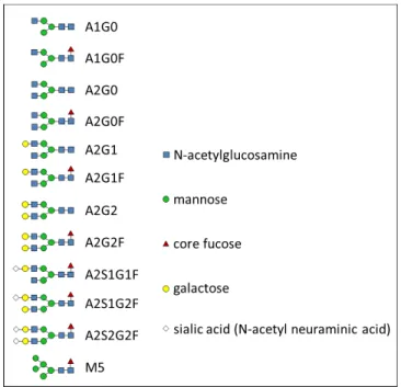
glycosylations illustrated in Figure 2.2.
Figure 2.2. Structures of common N-linked glycans examined in this manuscript.
BiopharmaLynx was not designed to process multidimensional data, so the software
processed the LC-CE-MS data as if it were LC-MS data. It identified each LC-CE-MS peak
as a separate component, assigning the same molecular mass and peptide identification to
data to help it identify peaks, but it was also not confused by the presence of multiple narrow
peaks with the same molecular mass. The relative abundance of each glycoform was
calculated by a manual summation of the total MS intensity for all peaks assigned to each
N-linked glycopeptide. The LC retention and CE migration times were found by generating a
separate 2D image plot using extracted ion chromato-electropherograms for each identified
N-linked glycopeptide. !
2.2.8 High MS Acquisition Rate LC-CE-ESI
To increase the data sampling rate in the MS dimension and to reduce undersampling
concerns, firmware modifications were made to a Waters Synapt G2 mass spectrometer
(Waters Corporation). The Synapt G2 is capable of performing a multi-dimensional
separation with a high MS acquisition rate: LC coupled with ion mobility spectrometry
(IMS) followed by MS detection. We repurposed the LC-IMS-MS functionality of the
instrument and performed LC-CE-MS. To accommodate a faster CE separation, a LC-CE
microchip was fabricated with a 4.3 cm separation channel. A schematic of the device can be
seen in Figure 2.3. Aside from the length of the separation channel, the dimensions and
operate of the device were very similar to those reported in Figure 2.1. The fabrication and
surface modification of the 10 cm and 4.3 cm devices were identical. For operation of the 4.3
cm device, voltages of +2.6, + 0, and + 6.6 kV were applied to the BGE, Waste, and EO
pump reservoirs, respectively. To inject sample into the separation channel, the voltages were
changed to +1.3, + 1.3, + 6.6 kV, respectively. A 40 ms CE injection was performed every 4
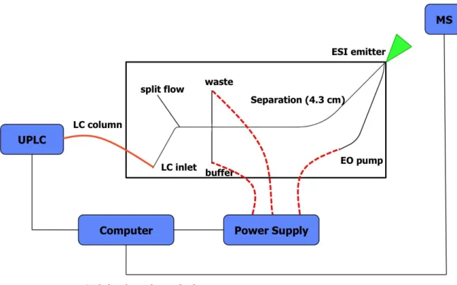
Figure 2.3. Schematic of the hybrid capillary LC-microchip CE-ESI experimental setup with a 4.3 cm long separation channel. The orange line represents a transfer capillary connecting the LC column to the microfluidic device. The dashed red lines represent electrical connections between the high voltage power supply and the microfluidic reservoirs.
The mass spectrometer scanned a range of 325 – 1600 m/z at an acquisition rate of 50
Hz. The sample used was a Waters MassPREP Protein Expression Mix (Waters Corporation),
which contained 400 nM bovine serum albumin, 100 nM enolase, 50 nM alcohol
dehydrogenase, and 25 nM phosphorylase B. The UPLC instrument, column, and mobile
phases were the same as reported earlier. The injection volume was 2 µL, the flowrate was 500 nL/min, and the gradient was 7 – 40% B in 15 min. Data were analyzed using the
2.3 Results and Discussion
2.3.1 Evaluation of System Performance
The LC-CE-MS system was evaluated for total peak capacity and reproducibility
using the 5-protein tryptic digest. For comparison this sample was separated by LC-MS and
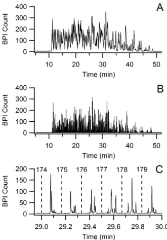
LC-CE-MS using identical LC conditions. The base peak ion count (BPI) chromatogram for
the LC-MS run is displayed along with the BPI chromato-electropherogram for an
LC-CE-MS run in Figure 2.4.
!!
The individual peaks of the LC-CE-MS run are too brief to see in Figure 2.3B, so a 1-min wide section of this run is displayed in Figure 2.4C. The peaks from sequential CE runs can be clearly seen, spaced by the 10 s period of the CE injections. Dashed lines indicate the
times at which the labeled CE injection number occurred. Because overlapping injections were used, the peaks are offset by 1 injection period. In other words, the first group of CE
peaks visible in Figure 2.4B came from injection number 173, and the peaks from injection number 179 are not visible in this figure. Figure 2.5 shows a two-dimensional image plot generated from the same data displayed in Figure 2.4B. This plot gives a better representation
of the power of this multidimensional separation. In this plot the color of the spots corresponds to the intensity of the base peak ion count. The position of each spot corresponds
!Figure 2.5. Image plot for the LC-CE-MS separation of a 5-protein tryptic digest mixture. This plot was generated from the same data shown in figure 2.3B.
Comparison of extracted ion chromatograms for the LC-MS and LC-CE-MS
separations of the 5-protein tryptic digest confirmed that the peptide bands had similar
temporal widths in both runs (Figure 2.6). Identical LC runs were performed using a standard
capillary spray tip interface and the microchip CE-ESI interface. By displaying a small m/z
range and aligning the traces, we can compare the observed peak widths for peptide bands
with and without the capillary to microchip transfer. Figure 2.6 shows that band widths and
shapes were very similar for LC-MS and LC-CE-MS indicating that the capillary to
separation of the 5 protein tryptic digest was used to estimate peak capacity for the LC
dimension of the LC-CE-MS run.
Figure 2.6. Extracted ion plots for the LC-MS (red) and LC-CE-MS (black) separations of the 5-protein tryptic digest. The LC-MS trace was shifted by +0.45 min to better align the peaks for better visual comparison; and the LC-CE-MS trace was shifted down by 20 counts to align the baselines.
The LC-MS BPI chromatogram contained too many unresolved peaks to accurately
measure peak widths, so an extracted ion chromatogram from a small m/z range (700 – 710)
was used. This chromatogram was processed with an open source software program (Peak
Finder, available at http://omics.pnl.gov/software) to estimate the median 4s peak width. A
total of 30 peaks were fit, yielding a median peak width of 16.5 s. To calculate peak capacity,
the full width of the LC separation window was determined from the LC-CE-MS data by
subtracting the run time of the first observed peptide peak (~11 min) from the run time of the
last observed peptide peak (~49 min). Dividing the LC separation window by the 4σ peak
processing the entire BPI chromato-electropherogram for the LC-CE-MS separation of the
5-protein tryptic digest using the same software program. A total of 334 peaks above a
threshold of 30 BPI were identified with a median peak width of 0.44 s. The average width of
the CE separation windows was estimated by visual examination of the image plot shown in
Figure 2.5 to be approximately 4.5 s. This average window divided by the median peak width
of 0.44 s, yielded an average CE dimension peak capacity of 10.2. Multiplying the estimated
peak capacities of the LC and CE dimensions yielded a total LC-CE peak capacity of
approximately 1400; over an order of magnitude greater than the LC-MS run with negligible
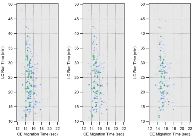
increase in analysis time. The reproducibility of the system was measured with 3 replicate
LC-CE-MS runs of the same 5 protein tryptic digest sample (Figure 2.7) performed on the
same day. The spot locations of ten randomly selected components were identified in the
image plots for each replicate run. For these 3 replicate runs, the average relative standard
deviations (RSD) for LC retention and CE migration times of these 10 spots were 0.32% and
Figure 2.7. Same day replicate LC-CE-MS separations of the 5 protein tryptic digest. The spot colors indicate base peak ion count.
2.3.2 N-linked Glycosylation Analysis of a Monoclonal Antibody
After characterizing the performance of the LC-CE-MS system, the same method
described above was applied to glycosylation profiling of a monoclonal antibody. The
molecule studied was an immunoglobulin G2 (IgG2) with two heavy chain N-linked
glycosylation sites, one in the Fc domain and one in the Fab domain. The sample was
prepared by digestion with trypsin, but was not chemically modified in any other way.
N-glycans were therefore attached to one of two tryptic peptides (EEQFNSTFR from the Fc
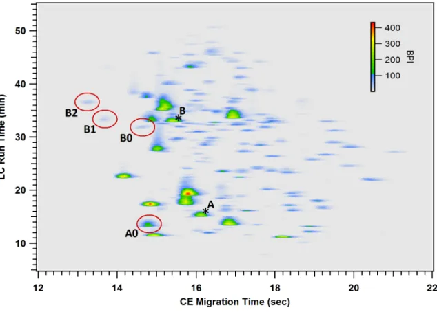
domain and NTSISTAYMELSSLR from the Fab domain). Figure 2.8 shows the 2D image
glycopeptides are circled on this plot. Unglycosylated tryptic peptides from each
glycosylation site were also observed.
Figure 2.8. Image plot for the LC-CE-MS separation of a digested IgG2 containing two N-linked glycosylation sites. The circled spots contained all of the observed N-linked glycopeptides. The spot labeled A0 contained all of the glyopeptides from the Fc domain site. Spots B0, B1, and B2 contained the glycopeptides from the Fab domain site containing 0, 1, and 2 sialic acid residues, respectively. The positions of corresponding unglycosylated peptides from each site are indicated with asterisks (*).
These two spots are not visible in Figure 2.8 because they were of low abundance and
they both coeluted with other highly abundant peptides. However, their locations, determined
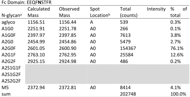
from extracted ion plots, are indicated by asterisks. Table 2.1 lists all of the observed
N-linked glycopeptides along with observed masses, locations in Figure 2.8, intensities, and
Table 2.1. N-linked glycopeptides observed by LC-CE-MS analysis of the IgG2 tryptic digest.
Fc#Domain:#EEQFNSTFR#
N1glycana#
Calculated#
Mass# Observed#Mass# Spot#Locationb#
Total# Intensity#
(counts)# %#total#of# aglyco# 1156.51# 1156.44# A# 539# 0.3%# A1G0# 2251.91# 2251.78# A0# 266# 0.1%# A1G0F# 2397.97# 2397.85# A0# 7613# 3.8%# A2G0# 2454.99# 2454.86# A0# 5479# 2.7%# A2G0F# 2601.05# 2600.90# A0# 154367# 76.1%# A2G1F# 2763.10# 2762.95# A0# 25584# 12.6%# A2G2F# 2925.15# 2924.98# A0# 486# 0.2%#
A2S1G1F# ## ## ## ## ##
A2S1G2F# ## ## ## ## ##
A2S2G2F# ## ## ## ## ##
M5# 2372.94# 2372.81# A0# 8414# 4.1%#
sum# ## ## ## 202748# 100.0%#
# # # # # #
Fab#Domain:#NTSISTAYMELSSLR#
N1glycan# Calculated#Mass# Observed#Mass# Spot#Location# Total#(counts)# Intensity# %#total#of# aglyco# 1671.81# 1671.73# B# 2926# 4.6%#
A1G0# ## ## ## ## ##
A1G0F# 2913.27# 2913.10# B0# 412# 0.6%#
A2G0# ## ## ## ## ##
A2G0F# 3116.35# 3116.20# B0# 12503# 19.5%# A2G1F# 3278.40# 3278.24# B0# 5187# 8.1%# A2G2F# 3440.45# 3440.29# B0# 1928# 3.0%# A2S1G1F# 3569.44# 3569.31# B1# 7254# 11.3%# A2S1G2F# 3731.55# 3731.37# B1# 13733# 21.4%# A2S2G2F# 4022.64# 4022.44# B2# 20310# 31.6%#
M5# ## ## ## ## ##
sum# ## ## ## 64253# 100.0%#
aGlycan!structures!are!defined!in!Figure!2.2.!
b!Spot!locations!correspond!to!Figure!2.8.!
!
A closer examination of the data displayed in Figure 2.8 and Table 2.1 indicates some
important features of this separation. First we can see that all of the N-linked glycopeptides
same horizontal or vertical position in the plot indicates that this would not have been the
case for a one-dimensional LC or CE separation. Second, we can see that the glycopeptide
spots are located in predictable regions relative to each other and their corresponding aglyco
peptides. Neutral glycosylations (spots A0 and B0) shifted the position relative to the aglyco
peptides (spots A* and B*) to earlier LC retention and CE migration times. As expected from
the greater relative change in molecular mass, the shift was greater for the smaller Fc domain
peptide (A). Except for the addition of a sialic acid residue, differences in N-glycan structure
had little effect on LC retention or CE migration. The addition of each sialic acid residue
caused a significant shift to earlier CE migration and later LC retention (spots B1 and B2
compared to B0). Finally, we can see significant differences in the glycosylation profiles of
the two different sites, as indicated by the different N-glycans observed in Table 2.1 as well
as the location of the glycans corresponding to A and B in Figure 2.5. This highlights the
importance of maintaining site specific information by analyzing glycosylation at the peptide
level.
There are more than 100 fully resolved spots visible in Figure 2.8. This clearly
indicates that far more information is available in this data than what has been analyzed here.
To fully exploit the power of this technology, improved data analysis software is needed. We
were able to generate 2D image plots from our LC-CE-MS data, but can only display a single
ion count (total ion, base peak, or extracted ion counts) as the color scale in these plots. To
access the wealth of MS data generated by this method we had to refer back to the linear raw
data file. We were not able to sum spectra in the 2D separation space. There are programs
designed for multidimensional gas chromatography (GCxGC)-MS (e.g. ChromaTOF, LECO