Representing statistical distributions for uncertain parameters in LCA. Relationships between mathematical forms, their representation in EcoSpold, and their representation in CMLCA

(1)

Uncertainties in LCA (Subject editor: Andreas Ciroth)

Representing Statistical Distributions for Uncertain Parameters in LCA

Relationships between mathematical forms, their representation in EcoSpold,

and their representation in CMLCA

Reinout Heijungs1_{* and Rolf Frischknecht}2

1_{Institute of Environmental Sciences (CML), Leiden University, POB 9518, 2300 RA Leiden, The Netherlands} 2_{ESU-services, Kanzleistrasse 4, 8610 Uster, Switzerland}

* Corresponding author ([email protected])

The incorporation of uncertainty calculations as a routine step in LCA requires the extension of databases and soft-ware that contain and support such information. The present advent of databases and software for LCA that support cal-culations with stochastic input data calls for a review of the most frequently assumed statistical distributions. These are

• the uniform distribution; • the triangular distribution;

• the normal or Gaussian distribution; • the lognormal distribution.

Although the mathematical form and properties of these dis-tributions are well-known, it is often problematic to connect theory, data, and software. One reason for this is that there is some freedom in choosing the parameters that describe these distributions. For instance, a uniform distribution can be de-scribed with a lowest and a highest value, or alternatively with a mean value and a width or half-width. Of course, getting the right uncertainty information and deciding which statisti-cal distribution is appropriate is difficult as well; this problem is, however, not addressed in this paper.

The purpose of this technical paper is to describe the rela-tionship between three representations:

• the mathematical form;

• the EcoSpold representation chosen by the ecoinvent database (an extensive LCA database that includes quantitative uncertainty information, see, e.g., Frischknecht et al. 2004);

• the representation chosen by the CMLCA software (an advanced LCA software tool that includes uncertainty analyses in a numeri-cal way – by Monte Carlo analysis – and in an analytinumeri-cal way – by formulae for error propagation).

Tables with cross-formulae enable a quick translation of one form into another form.

1 Representations

In this paper, three different representations of statistical distributions are used: the most often used mathematical form, the representation in EcoSpold, and the representa-tion in CMLCA. These three representarepresenta-tions should suffice to understand the relationships involved, and to add similar information for any other LCI database, set of LCIA char-acterization factors, or LCA software.

DOI: http://dx.doi.org/10.1065/lca2004.09.177

Abstract

Introduction. Statistical information for LCA is increasingly be-coming available in databases. At the same time, processing of statistical information is increasingly becoming easier by soft-ware for LCA. A practical problem is that there is no unique unambiguous representation for statistical distributions. Representations. This paper discusses the most frequently en-countered statistical distributions, their representation in math-ematical statistics, EcoSpold and CMLCA, and the relationships between these representations.

The distributions. Four statistical distributions are discussed: uniform, triangular, normal and lognormal.

Software and examples. An easy to use software tool is avail-able for supporting the conversion steps. Its use is illustrated with a simple example.

Discussion. This paper shows which ambiguities exist for speci-fying statistical distributions, and which complications can arise when uncertainty information is transferred from a database to an LCA program. This calls for a more extensive standardi-zation of the vocabulary and symbols to express such informa-tion. We invite suppliers of software and databases to provide their parameter representations in a clear and unambiguous way and hope that a future revision of the ISO/TS 14048 docu-ment will standardize representation and terminology for sta-tistical information.

Keywords:CMLCA; ecoinvent; EcoSpold, ISO-14048; lognormal distribution; normal distribution; statistical distributions; trian-gular distribution; uncertainties; uniform distribution

Introduction

(2)

1.1 The mathematical form

There is no unique mathematical representation. Apart from obvious differences in the choice of symbols in the formulae (like changing x into y), scales and origins may be shifted as long as this is done consistently. For instance, a uniform distribution may be described by a probability density func-tion having a non-zero value between a and b:

or equivalently by a probability density function having a non-zero value in a range that has a in its centre and a half-width of b:

Observe that the parameters a and b are used differently in these two formulae. In this paper, we have used the book by Morgan & Henrion (1990) for the representations in Section 2.

1.2 The EcoSpold representation

The ecoinvent parameters (see http://www.ecoinvent.ch/) are based on the EcoSpold format (see http://www.ecoinvent.ch/ download/EcoSpoldSchema_v1.0.zip), which again has its roots in the Spold 99 format (see http://www.spold.org/publ/ SPOLD99.zip). The EcoSpold format accommodates the following relevant keywords:

• uncertaintyType (field1_{3708; kind of uncertainty distribution)}

• meanValue (field 3707; (arithmetical) mean amount, further ab-breviated as MeanV)

• minValue (field 3795; minimum value, further abbreviated as MinV) • maxValue (field 3796; maximum value, further abbreviated as

MaxV)

• mostLikelyValue (field 3797; not used in ecoinvent data v1.1) • standardDeviation95 (field 3709; the square of the geometric

stand-ard deviation, and the double standstand-ard deviation for the lognormal, and normal distribution, respectively, further abbreviated as SD95).

1.3 The CMLCA representation

The CMLCA parameters (see http://www.leidenuniv.nl/cml/ ssp/software/cmlca/) are based on just three variables:

• value ((arithmetical) mean amount) • distribution (kind of uncertainty distribution) • uncertainty (some measure of dispersion)

This latter variable is labeled as follows:

• sigma (in case of normal distribution);

• width (in case of uniform and triangular distribution); • phi (in case of lognormal distribution).

The meaning of these variables will be explained later. As already mentioned, CMLCA includes analytical expres-sions for error propagation. These require, besides the mean

value, the variance s2_{of the distribution as a parameter. The}

next sections will therefore also contain expression for s2_in

terms of the (mean) value and the uncertainty parameter.

In addition to carrying out Monte Carlo simulations and using analytical formulae for error propagation, CMLCA also offers a way to add a generic uncertainty value to a large set of data items simultaneously. This is done on the basis of the coefficient of variation, which is defined as the dimensionless ratio between the distribution's standard de-viation and its mean:

With a fixed mean value, the dispersion parameter of the distribution is adjusted so as to satisfy

In other words, we need a formula of the form

width = f(value,CV)

for the uniform and triangular distribution,

sigma = f(value,CV)

for the normal distribution, and

phi = f(value,CV)

for the lognormal distribution. Concrete elaborations will be provided in the subsequent sections.

2 The distributions

This section will discuss the four statistical distributions that are most commonly used in the context of stochastic LCA: the uniform, triangular, normal and lognormal distributions.

2.1 The uniform distribution

The uniform distribution (see Morgan & Henrion 1990, p. 95) is a mathematically simple distribution. In EcoSpold, the keyword UncertaintyType has the value 4 to denote this dis-tribution. In CMLCA, it is the distribution that is listed as the second choice, and is represented as U(width).

It has a probability density function (Fig. 1) of the form

Its mean value is given by

and its variance by

1_{The 'field' is a unique identifier number, used in the documentation of}

the EcoSpold format.

(

)

2 12

1

2 _b _a

s = −

  

 _≤ _≤

− =

otherwise 0

1 )

(x _b _a a x b f

  

 ₋ _≤ _≤ ₊

=

otherwise 0

2 1 )

(x _b a b x a b

f

x s CV =

x CV s=

  

 _≤ _≤

− =

otherwise 0

1 )

(x _b _a a x b f

(

a b

)

x= +

(3)

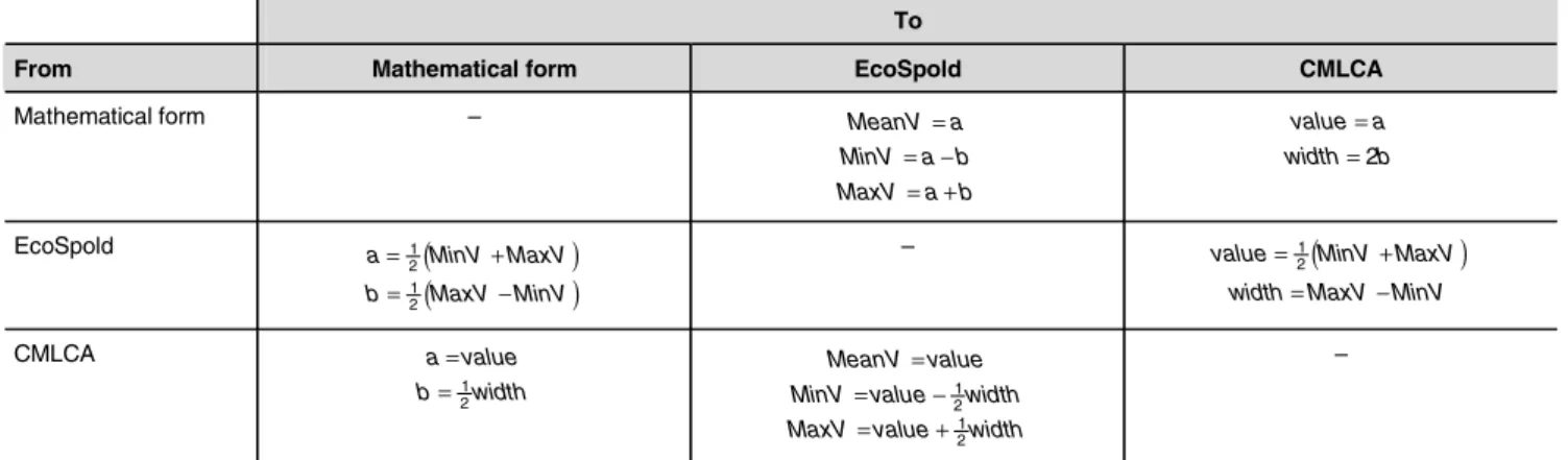
Table 1 shows how the parameters of the distribution, a and b, can be transformed into the parameters that are re-quired or provided by EcoSpold and CMLCA.

In CMLCA, the coefficient of variation translates into

For the variance we finally have

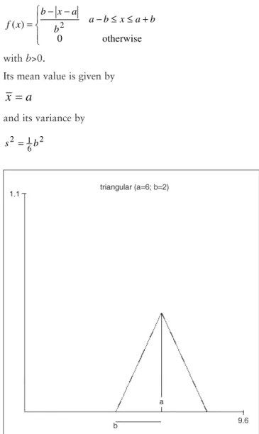
2.2 The triangular distribution

The symmetric triangular distribution2_{(see Morgan & Henrion}

1990, p. 96) is slightly more complicated than the uniform

distribution. In EcoSpold, the keyword UncertaintyType has the value 3 to denote this distribution. In CMLCA, it is the distribution that is listed as the third choice, and is repre-sented as T(width).

with b>0.

and its variance by

Fig. 1: The probability density function of the uniform distribution with pa-rameters a=4 and b=8

2_{Although ecoinvent in principle can accommodate an asymmetric} trian-gular distribution, it has been excluded from the discussion in this paper, because Morgan & Henrion (1990) do not discuss it, and because CMLCA does not support it.

To

From Mathematical form EcoSpold CMLCA

Mathematical form – 1

(

)

2

= +

= =

MeanV a b

MinV a

MaxV b

(

)

1 2

value a b

width b a

= +

= −

EcoSpold a MinV

b MaxV = =

–

(

)

*

1 2

value MinV MaxV

width MaxV MinV

= +

= −

CMLCA 1

2 1 2

a value width

b value width

= −

= + 1

2 1 2

MeanV value

MinV value width

MaxV value width =

= −

= +

–

*

Alternatively: value=MeanV

Table 1: Relationship between the representations for the uniform distribution

Fig. 2: The probability density function of the triangular distribution with parameters a=6 and b=2

value CV width=2 3× ×

2 12

1 2 _width

s =

   

+ ≤ ≤ − − − =

otherwise 0

)

( _b2 a b x a b

a x b x f

a

x

=

2 6 1

2 _b

(4)

Table 2 shows how the parameters of the distribution, a and b, can be transformed into the parameters that are re-quired or provided by EcoSpold and CMLCA.

For the variance we finally have

2.3 The normal distribution

The normal or Gaussian distribution (see Morgan & Henrion 1990, p. 88) looks mathematically more difficult than the uniform and triangular distributions, but is in fact easier to deal with. In EcoSpold, the keyword UncertaintyType has the value 2 to denote this distribution. In CMLCA, it is the distribution that is listed as the first choice, and is repre-sented as N(sigma).

with σ>0.

and its variance by

The ecoinvent documentation for the EcoSpold format gives as an explanation of the SD95 that it represents the double standard deviation, s:

The factor 2 is in fact the rounded value of 1.96, the two-sided critical value at significance level 0.95 from a table of the normal distribution (Abramowitz & Stegun 1972, p. 968).

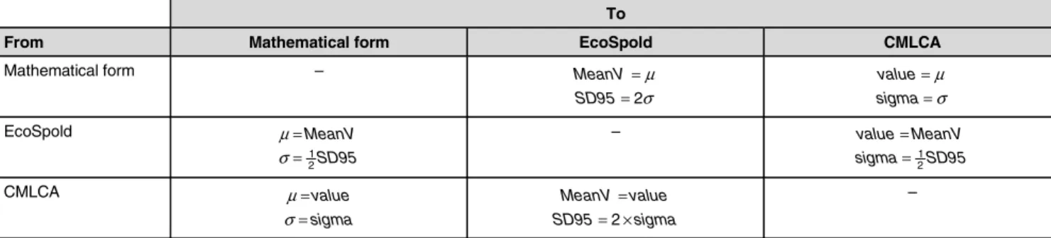
Table 3 shows how the parameters of the distribution, µ and _σ, can be transformed into the parameters that are re-quired or provided by EcoSpold and CMLCA.

For the variance we finally have To

Mathematical form – _MeanV _a

MinV a b

MaxV a b = = −

= +

2 value a

width b = =

EcoSpold

₍

₎

(

)

1 2 1 2

a MinV MaxV

b MaxV MinV

= +

= −

– 1

(

)

2

value MinV MaxV

width MaxV MinV

= +

= −

CMLCA

1 2

a value b width

=

= 1

2 1 2

MeanV value

MinV value width MaxV value width

=

= −

= +

–

Table 2: Relationship between the representations for the triangular distribution

Fig. 3: The probability density function of the normal distribution with pa-rameters µ=6 and σ=1

2 2 ₌_σ

s

s SD95=2

value CV

sigma= ×

2 2₌_σ

s value

CV width=2 6× ×

2 24

1 2 _width

s =

(

)

_



₋ ₋

= 2

2

2 1 exp 2

1 )

( µ

σ σ

π x

x f

µ

=

(5)

2.4 The lognormal distribution

The lognormal distribution (see Morgan & Henrion 1990, p. 89) is, due its asymmetry, more difficult than the other distributions discussed, both in its mathematics and in its interpretation. Nevertheless, it is an extremely often used distibution. In EcoSpold, the keyword UncertaintyType has the value 1 to denote this distribution; this is in fact the default value. In CMLCA, it is the distribution that is listed as the fourth choice, and it represented as L (phi).

with φ>0.

and its variance by

The ecoinvent documentation for the EcoSpold format gives as an explanation of the SD95 that it represents the square of the geometric standard deviation, SDg:

SD95 = SDg²

The exponent 2 is in fact the rounded value of 1.96, the two-sided critical value at significance level 0.95 from a ta-ble of the lognormal distribution. As most tata-bles do not specify the cumulative lognormal density, one should use the cumulative normal density (Abramowitz & Stegun 1972, p. 968), and perform a logarithmic transformation. The natu-ral logarithm of the geometric standard deviation is the stand-ard deviation of the natural logarithm of x (Strom & Stansbury 2000):

φ = ln(SDg)

For completeness of interpretation, we also provide formu-lae for the median

and the mode

x_mode = exp(ξ – φ²)

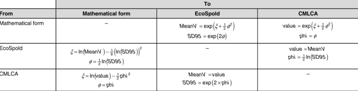
Table 4 shows how the parameters of the distribution, ξ and φ, can be transformed into the parameters that are re-quired or provided by EcoSpold and CMLCA.

so independent of value. For the variance we finally have

( )

(

2

)

2

2 _exp _phi ₁ _value

s = − ⋅

To

Mathematical form –

2 MeanV

SD95 µ σ = =

value

sigma µ σ =

=

EcoSpold

1 2

MeanV

SD95 µ σ = =

–

1 2

value MeanV

sigma SD95 =

=

CMLCA value

sigma µ σ =

= 2

MeanV value

SD95 sigma = = ×

–

Table 3: Relationship between the representations for the normal distribution

Fig. 4: The probability density function of the lognormal distribution with parameters _ξ=1 and _φ=0.3

( )

(

)

   

>

   



₋ ₋

=

otherwise 0

0 ln

2 1 exp 2

1 ) (

2

2 x x

x x

f _π_φ _φ ξ

(

2

)

2 1

expξ+ φ

=

x

( )

φ

(

exp

( )

φ 1

)

exp

( )

2ξ

exp 2 2

2 ₌ _⋅ ₋ _⋅

s

( )

ξ

exp

median =

x

(

1

)

ln 2₊

= CV

(6)

3 Software and Example

An easy to use software tool has been developed to assist us-ers of ecoinvent and/or CMLCA in translating and interpret-ing distributions and their parameters in the three representa-tions discussed here. Fig. 5 shows a screen shot of the user interface. The software tool can be downloaded from http:// www.ecoinvent.net/en/uncertainty.htm and from http:// www.leidenuniv.nl/cml/ssp/software/cmlca/distributions.html.

To illustrate the use of the tables and the software tool, we give an example. Suppose we have a data item that has been specified in EcoSpold as uncertaintyType=1; meanValue=10; standardDeviation95=1.2. To translate this into CMLCA-form, we use from Table 4 in Section 2.4 the formulae in the

fourth row and the fourth column (from EcoSpold to CMLCA). These formulae are:

Upon entering the values for meanValue and standard-Deviation95, we find value=10 and phi=0.0912. In the soft-ware tool, one selects the lognormal distribution and the EcoSpold-representation and clicks 'Edit parameters'. The values 10 and 1.2 are entered respectively. Then one changes the representation into CMLCA, and reads from the small table in the bottom left corner the values for 'value' and 'phi': 10 and 0.0912 respectively.

To

Mathematical form –

(

)

( )

2 1 2

exp

exp 2 MeanV

SD95

= +

= ξ φ

φ

(

)

2 1 2

exp value

phi ξ φ φ

= +

=

EcoSpold

(

)

(

)

(

)

2 1

8 1 2

ln ln

ln

MeanV SD95

SD95 ξ

φ

= −

=

–

(

)

1 2ln

value MeanV

phi SD95

= =

CMLCA

(

)

1 2

2

lnvalue phi

phi ξ

φ

= −

= exp 2

(

)

MeanV value

SD95 phi

=

= ×

–

Table 4: Relationship between the representations for the lognormal distribution.

(7)

4 Discussion

The importance of including uncertainty information into LCA has been recognized for more than a decade; see de Beaufort et al. (2003) for a review. Two main lines can be distinguished: the use of data quality indicators, and the use of statistical measures of dispersion, like standard deviations. A clear advantage of using data quality indicators is the possibility to capture uncertainty-related information that is difficult to quantify, such as the degree of data validation. An obvious advantage of quantitative information is the possibility to use methods from mathematical statistics to assess the uncertainty over the entire life cycle. Especially in large databases and advanced computer programs, the lat-ter type of analysis may be used for automatic uncertainty and sensitivity analyses. Experiences gained with ecoinvent Data v1.1 showed that primary information on variability and parameter uncertainty of unit processes due to e.g. meas-urement uncertainties, process specific variations, temporal variations is hardly available. A standardised procedure based on data quality indicators has been applied to over-come this shortcoming (Frischknecht and Heck 2004).

The EcoSpold format is an important and widely-used stand-ard for exchanging and reporting inventory data. There are other data formats as well. Perhaps the most important one is the one provided by ISO 14048 (Anonymous 2002). For-tunately, it contains fields (1.2.12) for including statistical information. But being primarily a data reporting format, it does not standardize the statistical vocabulary. This may lead to ambiguous and defective processing of the data files by software for LCA. The examples that illustrate the ISO/TS-14048 show that the field for name (ISO/TS 1.2.12.1) can be filled in many ways ('mean', 'mode', 'range', 'single point' are explicitly mentioned in ISO/TS 14048, Section 7.3, but the nomenclature is not mandatory), and that the same ap-plies to the name of the parameter field (Coefficient of vari-ance', 'Maximum value', 'Mean', 'Median', Minimum value', 'Sample size', 'Standard deviation', 'Estimated error'). To our regret, it is not possible to extend the translation that we provided between mathematics, EcoSpold and CMLCA to the ISO/TS-14048-data documentation format, unless a precise definition of the parameters that are supposed to represent the distributions has been established.

Interpretation of uncertainty information in data and results is an indispensable part of sound decision making and should be an integral part of the analysis itself. We hope that the present exposition stimulates and helps LCA-practitioners to apply uncertainty analyses in their practice of using LCA. Moreover, we hope that suppliers of LCA databases and software will take care to include uncertainty information and processing in their products. We invite these other sup-pliers to provide their parameter representations in a clear and unambiguous way, so that tables with translation for-mulae like the four above may be constructed. We also hope that a future revision of the ISO/TS 14048 document will put forward a standardized representation and terminology for statistical information. To what extent the representa-tions should be standardized is an open question.

References

Abramowitz M, Stegun IA (1972): Handbook of Mathematical Functions with Formulas, Graphs and Mathematical Tables. Dover Publications, Inc., New York

Anonymous (2002): Environmental Management – Life Cycle As-sessment – Data Documentation Format. ISO Technical Speci-fication ISO/DTS 14048, Geneva

de Beaufort-Langeveld ASH, Bretz R, van Hoof G, Hischier R, Jean P, Tanner T, Huijbregts MAJ (2003): Code of Life-Cy-cle Inventory Practice (includes CD-ROM). SETAC-Europe, Brussels

Copius Peereboom E, Kleijn R, Lemkowitz S, Lundie S (1999): Influence of inventory data sets on life cycle assessment re-sults. A case study on PVC. Journal of Industrial Ecology 2 (3) 109–130

Frischknecht R, Jungbluth N, Althaus H-J, Doka G, Dones R, Heck T, Hellweg S, Hischier R, Nemecek T, Rebitzer G, Spielmann M (2005): The ecoinvent Database: Overview and Methodological Framework. Int J LCA 10 (1) 3–9

Frischknecht R, Heck T (2004): Uncertainty Assessment in ecoinvent based on Data Quality Indicators and Basic Uncer-tainty Factors, poster presented at the 14th SETAC-Europe Annual Meeting, Prague, April 19

Huijbregts MAJ, Norris GA, Bretz R, Ciroth A, Maurice B, von Bahr B, Weidema BP, de Beaufort ASH (2001): Framework for Modelling Data Uncertainty in Life Cycle Inventories. Int J LCA 6 (3) 127–132

Huijbregts MAJ, Gilijamse W, Ragas AMJ, Reijnders L (2003): Evaluating uncertainty in environmental Life-Cycle Assessment. Environmental Science and Technology 37, 2600–2608 Huijbregts MAJ, Heijungs R, Hellweg S (2004): Conference

Re-ports: 2nd Biannual Meeting of iEMSs. Complexity and inte-grated resources management: Uncertainty in LCA. Osnabrück, June 14–17, 2004. Int J LCA 9 (5) 341–342

Maurice B, Frischknecht R, Coelho-Schwirtz V, Hungerbühler K (2000): Uncertainty analysis in life cycle inventory. Applica-tion to the producApplica-tion of electricity with French coal power plants. Journal of Cleaner Production 8, 95–108

Meier MA (1997): Eco-efficiency evaluation of waste gas purifi-cation systems in the chemical industry. Ecoinforma Press, Bayreuth

Morgan MG, Henrion M (1990): Uncertainty. A Guide to Deal-ing with Uncertainty in Quantitative Risk and Policy Analysis. Cambridge University Press, Cambridge

Sonnemann GW, Schuhmacher M, Castells F (2003): Uncertainty assessment by a Monte Carlo simulation in a life cycle inven-tory of electricity produced by a waste incinerator. Journal of Cleaner Production 11, 279–292

Strom DJ, Stansbury PS (2000): Determining Parameters of Log-normal Distributions from Minimal Information. American Industrial Hygiene Association Journal 61, 877–880 http://www.ecoinvent.ch/

http://www.ecoinvent.ch/download/EcoSpoldSchema_v1.0.zip http://www.leidenuniv.nl/cml/ssp/software/cmlca/

http://www.spold.org/publ/SPOLD99.zip http://www.ecoinvent.net/en/uncertainty.htm

http://www.leidenuniv.nl/cml/ssp/software/cmlca/distri butions.html