LEARNING WITH MORE DATA AND BETTER MODELS FOR VISUAL SIMILARITY AND DIFFERENTIATION
Xufeng Han
A dissertation submitted to the faculty of the University of North Carolina at Chapel Hill in partial fulfillment of the requirements for the degree of Doctor of Philosophy in the Department of
Computer Science.
Chapel Hill 2016
©2016 Xufeng Han
ABSTRACT
Xufeng Han: Learning with More Data and Better Models for Visual Similarity and Differentiation (Under the direction of Alexander C. Berg)
This thesis studies machine learning problems involved in visual recognition on a variety of computer vision tasks. It attacks the challenge of scaling-up learning to efficiently handle more training data in object recognition, more noise in brain activation patterns, and learning more capable visual similarity models.
For learning similarity models, one challenge is to capture from data the subtle correlations that preserve the notion of similarity relevant to the task. Most previous work focused on improving feature learning and metric learning separately. Instead, we propose a unified deep-learning modeling framework that jointly optimizes the two through back-propagation. We model the feature mapping using a convolutional neural network and the metric function using a multi-layer fully-connected network. Enabled by large datasets and a sampler to handle the intrinsic imbalance between positive and negative samples, we are able to learn such models efficiently. We apply this approach to patch-based image matching and cross-domain clothing-item matching.
For analyzing activation patterns in images acquired using functional Magnetic Resonance Imaging (fMRI), a technology widely used in neuroscience to study human brain, challenges are small number of examples and high level of noise. The common ways of increasing the signal to noise ratio include adding more repetitions, averaging trials, and analyzing statistics maps solved based on a general linear model. In collaboration with neuroscientists, we developed a machine learning approach that allows us to analyze individual trials directly. This approach uses multi-voxel patterns over regions of interest as feature representation, and helps discover effects previous analyses missed.
ACKNOWLEDGMENTS
I would like to thank my advisor, Dr. Alex Berg, for his guidance and support over the earlier years Stony Brook and later at UNC. I am also grateful to Dr. Tamara Berg, a long-term collaborator and an inspiring mentor. I would also like to thank my thesis committee, for their thoughtful suggestions and helpful criticism, all to make this dissertation a better work.
I feel fortunate and honored to get involved in a number of exciting projects along the way, and I am very grateful to the following collaborators for the knowledge, help and joy they brought to me: Thomas Leung, Yangqing Jia, Rahul Sukthanka, Dave Silver and Abhigit Ogale, during my two internships at Google; Lukas Marti, during a fun and fruitful summer at Apple; Hoi-chung Leung, during our challenging fMRI analysis collaboration; Kota Yamaguchi, Karl Stratos, Margret Mitchell, Hal Daume III, Amit Goyal, Jesse Dodge and Alyssa Mensch, during an inspiring summer workshop at Johns Hopkins University; Rita Goldstein, Nelly Alia-Klein, Muhammad Parvaz, and Tom Maloney, during my adventurous trips to the Brookhaven National Laboratory.
I am proud to be a member of the Berg’s group. Over the years I have had the fortune to know, work with and even share a house with some of the amazing members in the group, especially Kota Yamaguchi, Vicente Ordonez, Wei Liu, Hadi Kiapour, Sirion Vittayakorn, and Eunbyung Park.
I would also like to thank mentors and friends from Stony Brook, especially Dr. Dimitris Samaras, Jean Honorio, Yun Zeng, Kiwon Yun, and Yifan Peng, Hojin Choi, and Chen-ping Yu, for making my early PhD years eventful and memorable.
Also thanks to my office mate, Yunchao Gong, as well as members of the V3D Lab at UNC, especially Dr. Jan-Michael Frahm, Jared Heinly, Johannes Schoenberger, Ke Wang, Dinghuang Ji and Enliang Zheng for all the interesting discussions we had.
Special thanks to Ms. Jodie Gregoritsch for all the administrative assistance from months before I arrive at UNC to the last days I am here.
TABLE OF CONTENTS
LIST OF TABLES . . . x
LIST OF FIGURES . . . xi
1 INTRODUCTION . . . 1
1.1 Motivation . . . 1
1.2 Thesis Statement . . . 5
1.3 Contributions . . . 7
1.3.1 MatchNet . . . 7
1.3.2 Exact Street-to-Shop . . . 8
1.3.3 Multi-Voxel Pattern Analysis . . . 8
1.3.4 DCMSVM . . . 8
2 VISUAL SIMILARITY LEARNING USING DEEP NEURAL NETWORKS . . . 10
2.1 Introduction. . . 10
2.2 Similarity Learning for Patch-based Image matching . . . 11
2.3 Background and Prior Work . . . 12
2.4 Deep Neural Network Architecture . . . 14
2.5 Algorithms for Learning and Prediction . . . 16
2.5.1 Reservoir Sampling for Label Balancing . . . 17
2.5.2 A Two-Stage Prediction Pipeline . . . 19
2.6 Evaluation on Image Patch Matching . . . 20
2.6.1 Dataset and Evaluation Protocol . . . 20
2.6.3 Variations of MatchNet . . . 21
2.6.4 Results and Discussion . . . 22
2.7 Cross-domain Similarity for Exact-Match Clothing Item Retrieval . . . 25
2.7.1 Exact Street to Shop . . . 25
2.7.2 Item Localization . . . 25
2.7.3 Similarity Learning . . . 26
2.8 Evaluation on Exact-Match Clothing Item Retrieval . . . 29
2.8.1 Dataset and Evaluation Protocol . . . 29
2.8.2 Main Results . . . 31
2.9 Summary . . . 34
3 MULTIPLE-VOXEL PATTERN CLASSIFIER LEARNING FOR FMRI IMAGES . . . 35
3.1 Introduction. . . 35
3.2 Behavioral Tasks and Image Data . . . 37
3.2.1 Working Memory and Localizer Tasks . . . 37
3.2.2 Image Data Acquisition, Preprocessing and Defining ROIs . . . 38
3.3 Multiple-Voxel Pattern Analysis . . . 40
3.3.1 Model and Features . . . 40
3.3.2 Cross-validation . . . 41
3.4 Results and Discussion . . . 41
3.4.1 Classification of Activation Patterns during Probe Recognition . . . 41
3.4.2 Classification of Activation Patterns during Selective Maintenance . . . 43
3.4.3 Classification of Activation Patterns in other Visual Association Regions . . . 45
3.5 Discussion . . . 47
3.6 Summary . . . 50
4 DISTRIBUTED PARALLEL LEARNING FOR OBJECT RECOGNITION . . . 51
4.1 Introduction. . . 51
4.3 Parallelizing Multi-class Linear SVM Learning using Consensus Optimization . . . 55
4.3.1 Consensus Formulation of the Learning Problem . . . 55
4.3.2 Alternating Direction Method of Multipliers for Consensus Optimization . . . 56
4.3.3 A Sequential Dual Solver for the Sub-problem . . . 58
4.4 Evaluation . . . 59
4.4.1 Time-Accuracy Trade-off under Different Number of Splits . . . 61
4.4.2 Convergence and Regularization . . . 62
4.4.3 Early Stopping . . . 63
4.4.4 High Dimensional Image Features . . . 64
4.4.5 Unbalanced Training Set . . . 64
4.5 Summary . . . 64
5 CONCLUSION . . . 66
5.1 Summary of Results . . . 66
5.1.1 MatchNet . . . 66
5.1.2 MVPA . . . 67
5.1.3 DCMSVM . . . 68
5.2 Closing Remarks . . . 68
A DERIVATION OF DCMSVM SUB-PROBLEM AND ITS SEQUENTIAL DUAL SOLVER . . 69
A.1 Dual derivation of DCMSVM subproblem . . . 69
A.2 Sequential dual method for the subproblem . . . 72
LIST OF TABLES
2.1 Layer specification of MatchNet. . . 15
2.2 Patch matching results on UBC dataset . . . 22
2.3 Accuracy vs. quantiazation tradeoff. . . 24
2.4 Statistics of the training and validation sets for similarity learning. . . 27
2.5 Test dataset statistics and top-20 item retrieval accuracy. . . 32
3.1 Average accuracy in classification of activation patterns of the FG and PHG across time (early, middle and late) for face and scene probes. . . 42
LIST OF FIGURES
1.1 The representation model and the decision model . . . 2
1.2 Illustration of different representation models for face detection. . . 4
2.1 Illustration of the MatchNet architecture. . . 14
2.2 Visualization of the learned first-layer convolution filters. . . 17
2.3 Visualization of activations in the feature network triggered from an input patch. . . 17
2.4 A Two-Stage prediction pipeline for computing pairwise matching score. . . 19
2.5 Accuracy vs. feature dimension tradeoff. . . 23
2.6 Illustration of the training and fine-tuning procedure. . . 28
2.7 Examples of street photos and photos . . . 30
2.8 A screenshot of an example post in ModCloth’s Style Gallery. . . 30
2.9 Example retrievals using category-specific similarity. . . 33
2.10 Top-kitem retrieval accuracy for differentk. . . 33
3.1 Visual working memory task with a selection cue. . . 36
3.2 Average percent signal change in fMRI signal across time in regions associated with face and scene processing during the working memory task. . . 38
3.3 Functionally defined regions of interest. . . 39
3.4 Mean accuracy in classification of face/scene during selective maintenance and probe recognition using voxels in the FG and ventral PHG. . . 42
3.5 Mean accuracy in classification of face/scene during selective maintenance. . . 44
3.6 Mean accuracy in classification of face/scene during selective maintenance (A) and probe recogni-tion (B) using voxels in regions associated with face and scene processing as shown in previous studies. . . 46
4.1 Image classification performance on LSVRC100 and LSVRC1000. . . 61
4.2 Time-Accuracy Trade-off under different number of splits. . . 62
CHAPTER 1
INTRODUCTION 1.1 Motivation
We need to imagine no further than a coffee shop scenario to see that visual similarity and differenti-ation are applied in the human vision system every day.
To make a medium coffee, a barista picks the topmost cup from a stack of medium-sized paper cups on the busy counter and turn to the coffee machine.
Before the barista reaches for the cup, the ability to differentiate medium cups from other objects and from cups of other sizes allows her to focus on the right target. At the same time, the ability to match local parts of the images projected into each eye helps her figure out the distance to the cup and plan for the reach.
Inspired by the human vision system, an interesting question is how to make computer vision systems process visual similarity and achieve visual differentiation. Such systems have merit in at least the following three aspects: (1) the ability to differentiate between objects will improve human-computer interaction. A robot with vision could understand what is around it and who it is interacting with much easier than a robot with just speech could, because the user no longer needs to describe everything. (2) They provide models and tools for understanding how the human vision system works. For example, a recent work (Gatys et al., 2015) models artistic style perception in paintings as the correlations of internal filters responses at different processing layers within a neural network trained for object classification. The model is validated by generating highly convincing renderings of an image in the style of different painters. (3) They attract scientific and engineering effort that makes faster, more accurate, and more reliable systems than the human vision system.
Visual Similarity
Original Representation
Transformed Representation
Visual Differentiation
…
Decision Output (e.g. similarity, scores for different options)
1010…110 1110…010
0.98
111101011…01010
Umbrella
0.9 Flamingo 0.5 Skirt 0.4
…
Decision Model
Representation Model
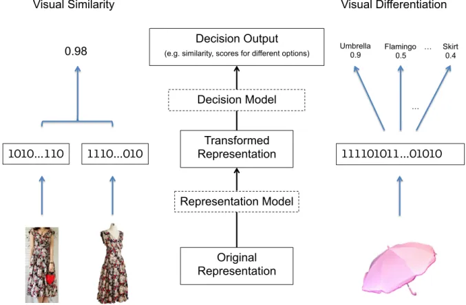
Figure 1.1: The representation model and the decision model for visual similarity and differentiation. On the left, two photos of dresses are first transformed from pixels into feature vectors, and then compared based on a decision model to obtain a similarity score. On the right, a photo of an object is also transformed from pixels into a feature vector before the decision model can compute a score for each possible labels. This thesis is concerned with identifying and tackling the challenges in designing the two types of models and learn them efficiently as we have more and more data.1
relevant to the task and by reducing irrelevant nuances in the original representation. The decision model encodes knowledge of how to reason about the transformed representation and produce results required by the task. Figure 1.1 shows a diagram of the two models connected together, as well as an illustration of how systems for visual similarity and differentiation can be viewed in this way.
For both visual similarity and visual differentiation, the state-of-the-art systems use machine learning to build the representation model and the decision model. The idea is to consider those models as functions, which either map a vector to a scalar or to another vector, and represent the functions in a certain parameter space. This way, building a model becomes estimating parameters such that not only
1
does the model fit existing observations (training data) but also works for unseen, future, observations – also calledtest data.
An alternative to using machine learning throughout is to start with good intuition of the data and knowledge of the task to design the majority of each model by hand and leave a small number of hyper-parameters to be tuned quickly on a small validation dataset. For example, we can represent an image using its color histogram. This transforms the original pixel-value representation into a fixed-length vector representation, where each element in the vector is the proportion for each base color. The choice of color space (e.g. RGB, HSI, Lab, etc.) and the way we divide it can be predetermined based on domain knowledge, and assuming the whole space is covered (so all colors count), we only need to decide on one free parameter: the number of base colors. This representation may work quite well if the task is to distinguish between oranges and apples. For this task, it is harmless that the transformed representation loses most information on the spatial distribution of the colors, but for other tasks it could matter a lot.
Much research has been done on making the representation models robust to irrelevant variations in the image and work for general domains. Along the way, many effective approaches have been cleverly hand-crafted, which helped various visual similarity and differentiation tasks, for example, SIFT descrip-tor for matching local images (Lowe, 2003), filter banks representation for texture classification (Leung & Malik, 2001), spatial pyramid pooling for object retrieval and scene classification (Lazebnik et al., 2006), locally-constrained linear coding for robust object recognition (Yu et al., 2009; Wang et al., 2010), Histogram of Oriented Gradients (HOG) template for object detection (Dalal & Triggs, 2005), etc.
Hand-crafted representation models are fundamentally biased and thus is difficult to benefit from more data. More samples may provide a better prior distribution in the space of the transformed representation, but the effect on the overall performance is often uncertain, either because a better prior may only amplify the bias of the representation model, or because the learning algorithm for the decision model may assign a higher weight to the goodness-of-fit on the data than to the prior distribution.
A B C D
…
E
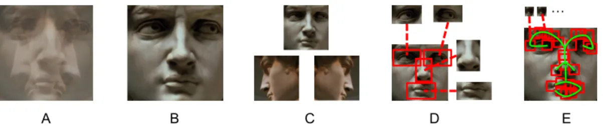
Figure 1.2: Illustration of different representation models for face detection compared in Zhu et al. (2015). Here we simply use the face of Michelangelo’s David to represent appearance templates, knowing that actual templates are in HOG space. (A)A single rigid template. (B)A single rigid template learned on frontal faces. (C)Mixture models for the whole face. (D)Deformable Parts Models (DPM).(E) DPM with tree configuration for parts and supervised part locations (on facial landmarks). Detection performance increases (A<B<C<D<E) as the representation model has more and more capacity to model variance of appearance in the data (C, D and E), and as better prior knowledge is used (B and E).
dot-products) between templates and HOG features from corresponding parts. In Figure 1.2 we illustrates some of the face models compared in their paper. Since there are frontal faces as well as profile ones in the dataset, a single rigid model trying to encode them all perform the worst, whereas one tuned for the just the frontal faces perform better — proper bias helps. A mixture of rigid templates have enough capacity to model different views separately and thus perform better than either one above. However the performance saturates quickly when the amount of training samples increases, because these models are too biased to handle the total variance of facial appearance. Deformable Parts Models (DPM) (Felzenszwalb et al., 2010) can model the object with several movable parts whose center positions form a star-shaped or tree-shaped (Yang & Ramanan, 2013; Zhu & Ramanan, 2012) spatial configuration. Since the parts are allowed to move around, more accurate appearance models can be learned. The configuration is also parameterized (e.g. as 2D Gaussian distributions of relative location for each part) and can either be learned. As expected, DPMs outperform rigid template mixtures. The intuition here is that a rigid template is good at handle local appearance variance between faces at part scale, but insufficient to model the variance in configurations of parts, which DPMs can model separately. Moreover, the authors show that models learned with supervising the part location using facial landmarks (e.g. tip of the nose, corners of eyes, etc) perform the best, which demonstrated again that good prior helps when applied properly.
demonstrated directly using HOGgles (Vondrick et al., 2013), is that in the space of HOG template, albeit high dimensional, transformed random natural background patches could be very similar to actual objects.
To overcome similar limitations with hand-crafted representation models, much research has been done on learning representation models directly from pixels. A very influential model is the AlexNet (Krizhevsky et al., 2012), a multiple-hidden-layer (deep) neural network, in which each layer performs a differentiable non-linear transformation on the output of the previous layer. The layers can be one of the following types: convolution with Rectified Linear Unit (ReLU)2as activation, max-pooling, normalization and affine transformation followed by ReLU3. This model won the ILSVRC’12 Image Classification Challenge and pushed visual differentiation to new state-of-the-art.
1.2 Thesis Statement
Visual similarity concerns the identity relation between two visual entities. A similarity model maps two visual entities in certain representations to a scalar value, which indicates the, e.g. semantic, difference/similarity between the two. Visual differentiation concerns the identity relation between a visual entity and a concept. A differentiation model maps a visual entity to a vector whose elements indicate the strength of the identity relation between the entity and a set of predefined concepts.
To fully exploit the increasing amount of data available for visual similarity and differentiation, we need to address various challenges in seeking models that scale with the data and seeking algorithms that scale with both. One of them is how to design the space of similarity models such that both the representation model and the decision model benefit from the data together. Most previous work on visual similarity learning fix one and improve the other. We argue that jointly training the two scales better with the data, and developed such a model using deep convolutional neural networks for the task of local image patch matching. An associated challenge is how to make use of potentially quadratic number of pairs from a list of entities in an efficient way in terms of both space and time. We propose a sampling approach, which avoids explicitly generating training pairs (space efficient) and also avoids random reading of the database (time efficient).
2ReLU(x) = max(0, x)
3
Also called “fully-connected” layer, since every node in the output layer outputs a weighted sum of every node in the input
Another challenge happens when similarity models are applied in a retrieval setting, where the meaning of “relevant” is strict (e.g. finding the exact dress from a picture taken with a phone among a million stock photos) and a generic similarity model may not be sufficient. The training pairs might not be easy to collect too. The challenge is to design a training algorithm that can deal with limited data at an early stage and kickstart a positive feedback loop. We propose to use deep neural network models for both its ability to approximate non-linear mappings (a good property for decision models), and its potential to couple with a neural representation model. We also propose to train models only on a short list of candidates to alleviate data imbalance.
More data can mean more dimensions rather than more independent samples. For example, functional magnetic resonance imaging (fMRI) allows neural scientists to measure activity of different brain regions while the subject is performing a certain task, but it is expensive to run fMRI. Therefore most study involves only a small number of subjects, each going through a small number of “trials”. On the other hand, a brain scan can have105voxels. Moreover, the measurement is prone to subject’s head motion and is quite noisy. In such cases, choosing a good bias in the vast space of potential representation and decision models is crucial. We propose a system that combines domain knowledge, regularization, linear max-margin model and cross-validation for an fMRI study of visual working memory.
For visual differentiation, both the number of concepts and the number of samples for each concept can grow. When the total amount of data too large enough to be hold in memory on one machine, not only the model but the learning algorithm as well will need to scale with the data. The challenge is how to distribute the computation involved in the decision model to different machines. One aspect of the challenge is how to formulate the original problem as connected subproblems; another aspect is how to solve the subproblems efficiently. We study this problem in the context of multi-class support vector machine for large scale object recognition, and propose a principled approach using consensus optimization to address the first aspect, and a sequential dual solver to address the second.
Motivated by the above considerations, the main thesis that this dissertation aims to support is the following:
increase in data imbalance, increase in the dimension of representation and increase in noise. It can be achieved through (1) joint feature and metric modeling using neural networks, (2) systematic model selection, and (3) objective reformulation for data parallelization using consensus optimization.
1.3 Contributions
In this section, we briefly summarize the contributions presented in the following chapters.
1.3 MatchNet
As its name suggests, MatchNet is neural network for image matching. Following the theme of this thesis, we make use of large patch datasets to learn both the representation model and the decision model for the task of matching local image patches. Both models consist of layers of neural networks, which allows us to build an end-to-end training system from raw image patches to “match/non-match” labels using standard error back-propagation.
The original patch dataset comes with groups of matching matches as well as some fixed set of non-matching patches. Instead of using the predefined set, we develop a sampling approach to generate non-matching pairs (negatives) on the fly during training. This significantly increases the quantity and variety of negative pairs, and also allows us to balance the label distribution. The sampler keeps a buffer in the memory, and thus eliminating the need of random access to the entire database in search of negative pairs, making the learning compatible with mini-batch stochastic gradient descent in a streaming training setting.
MatchNet achieves state-of-the-art matching performance in terms of accuracy. We cite relevant previous results and run home brew baseline comparisons to show that coupling feature and metric learning indeed helps.
1.3 Exact Street-to-Shop
Exact Street-to-shop is a retrieval task of finding in large amount of stock photos exact items in a query consumer photo. It requires highly specific similarity models across the two domains:street photos andshop photos. One important characteristic of the shop photos is that we do not know where the item of interest is, and in many cases there are multiple items in single image. Therefore localization of the item becomes particularly important. Nonetheless, localization of clothing item is an open research problem by itself. One of our contribution is showing that applying an off-the-shelf high-recall localization method “over-generate” item candidates in every shop photos followed by a coarse retrieval and a fine reranking
can be quite effective.
Another contribution is on the similarity model. Although in our experiment the course retrieval step uses a fixed representation models, the fine reranking step employ a learned decision model model specifically trained for the exact matching task. Both the representation model and the decision model are neural network based, so when more data comes in the future, we can easily switch on back-propagation in the representation model to make it learnable, just like in MatchNet. Therefore this approach has the potential to scale well with more data.
1.3 Multi-Voxel Pattern Analysis
This is a differentiation task in the space of fMRI images. This is a successful collaboration with neural scientists who use fMRI to study selective maintenance4in human visual working memory. One contribution is that machine learning with voxel activity patterns helps reveal selective maintenance in several regions where scientists predicted it exists but has not confirmed by using traditional methods of analysis. Another contribution is that we demonstrate that combining feature selection, regularization, linear max-margin model and cross-validation can make effective use of information in the fMRI dataset where the dimension of representation is high, the sample size small and the signal noisy.
1.3 DCMSVM
We propose a new algorithm named Distributed Consensus Multiclass SVM (DCMSVM) for efficient distributed parallel training of “single machine” or direct multi-class support vector machines, making
4
CHAPTER 2
VISUAL SIMILARITY LEARNING USING DEEP NEURAL NETWORKS5 2.1 Introduction
Solutions to many computer vision problems rely on computing the similarity between pairs of visual entities. At the scale of local image patches around key points (e.g. corners), computing the similarity between patches leads to putative matching of key-points, which can be used for testing whether two images are geometrically related, and if they are, computing the transformation between them. Similarity can also be computed at object scale for retrieving from an objects database instances that match or are similar to a given query.
An interesting and challenging aspect of computing similarity that the notion of similarity is task-dependent. For example, we might consider a white dog more similar to a gray wolf than to a white cat, even though the color of the dog and the cat are more similar. Assuming collecting labeled data for the task is either necessary or relatively straightforward compared to crafting a customized similarity, this task-dependent nature calls for a data-driven approach posted as the following learning problem: given a dataset where pairs between elements are either implicitly or explicitly labeled as matching (very similar) or non-matching (not so similar), how to learn a pair-wise function that models a notion of similarity that conforms to the train data and generalizes in the given domain.
In this chapter, we begin by proposing a deep neural network model and a learning approach in the context of image patch matching. We demonstrate that coupling the learning of feature representation and distance metric is effective. Finally we present an application of such model in the context of exact-match clothing item retrieval.
5
2.2 Similarity Learning for Patch-based Image matching
Patch-based image matching is used extensively in computer vision. Finding accurate correspon-dences between patches is instrumental in a broad variety of applications including wide-baseline stereo (e.g., (Matas & Chum, 2004)), object instance recognition (e.g., (Lowe, 1999), fine-grained classification (e.g., (Yao et al., 2012)), multi-view reconstruction (e.g.(Seitz et al., 2006)), image stitching (e.g.(Brown & Lowe, 2007)), and structure from motion (e.g.(Molton et al., 2004)).
Since 1999, the advent of the influential SIFT descriptor (Lowe, 1999), research on patch-based matching has attempted to improve both accuracy and speed. Early efforts focused on identifying better affine region detectors (Mikolajczyk et al., 2005), engineering more robust local descriptors (Mikolajczyk & Schmid, 2005; Heinly et al., 2012), and exploring improvements in descriptor matching using alternate distance metrics (Jain et al., 2012; Jia & Darrell, 2011).
Early efforts at unsupervised data-driven learning of local descriptors (e.g., (Ke & Sukthankar, 2004)) were typically outperformed by modern engineered descriptors, such as SURF (Bay et al., 2006), ORB (Rublee et al., 2011). However, the greater availability of labeled training data and increased computational resources has recently reversed this trend, leading to a new generation of learned descriptors (Brown et al., 2011; Trzcinski et al., 2012, 2013; Simonyan et al., 2014) and comparison metrics (Jia & Darrell, 2011). These approaches typically train a nonlinear model discriminatively using large datasets of patches with known ground truth matches and serve as motivation for our work.
Concurrently, approaches based on deep convolutional neural networks have recently made dramatic progress on a range of difficult computer vision problems, including image classification (Krizhevsky et al., 2012), object detection (Erhan et al., 2014), human pose estimation (Toshev & Szegedy, 2014), and action recognition in video (Karpathy et al., 2014; Simonyan & Zisserman, 2014). This line of research highlights the benefits of jointly learning a feature representation and a classifier (or distance metric), which to our knowledge has not been adequately explored in patch-based matching.
Euclidean distance, in MatchNet, the representations are compared using a learned distance metric, implemented as a set of fully connected layers.
Our contributions include: 1) A new state-of-the-art system for patch-based matching using deep convolutional networks that significantly improves on the previous results. 2) Improved performance over the previous state of the art(Simonyan et al., 2014) using smaller descriptors (with fewer bits). 3) A careful set of experiments using standard datasets to study the relative contributions of different parts of the system, showing that MatchNet improves over both hand-crafted and learned descriptors plus comparison functions. 4) Finally we provide a public release of MatchNet trained using our own large collection of patches.
2.3 Background and Prior Work
Much previous work considers improving some components in the detector-descriptor-similarity pipeline for matching patches. Here we address the most related work that considers learning descriptors or similarities, organized by goal and the types of non-linearity used.
multiple convolutional and spatial pooling layers plus an optional bottle neck layer to obtain feature vectors, followed by a similarity measure also based on neural nets.
Metric learning methods such as (Jain et al., 2012) and (Jia & Darrell, 2011) learn a similarity function between descriptors that approximates a ground truth notion of which patches should be similar, and achieve results that improve on simple similarity functions, most often the Euclidean distance. Jain et al. (Jain et al., 2012) introduces non-linearity with a predefined kernel on patches. A Mahalanobis metric is learned on top of that similarity. Jiaet al. (Jia & Darrell, 2011) uses a parametric distance based on a heavy-tailed Gamma-Compound-Laplace distribution, which approximates the empirical distribution of elements in the difference of matching SIFT descriptors. The parameters for this distance are estimated using the training data. In comparison, we use a two-layer fully connected neural network to learn the pairwise similarity, which has the potential to embrace more complex similarity functions beyond distance metrics such as Euclidean.
Semantic hashing or embedding learning methods learn non-linear mappings to generate low di-mensional representations, whose similarity in some easy-to-compute distance metric (e.g., Hamming distance) correlates with the semantic similarity. This can be done using neural networks, e.g., (Chopra et al., 2005) and (Salakhutdinov & Hinton, 2007) with a two-tower structure and recently (Wang et al., 2014) that samples triplets for training. Spectral hashing (Weiss et al., 2008) or boosting (Shakhnarovich, 2006; Trzcinski et al., 2013) can also be used to learn the mapping. This approach can be applied to raw image input (Salakhutdinov & Hinton, 2007) as well as to local feature descriptors (Strecha et al., 2012). In comparison, although we do not map input to an intermediate embedding space explicitly, the representation provided by our feature extraction network naturally serves the purpose, and the dimensionality can be controlled depending on the accuracy vs. storage and computation tradeoff. We explore and analyze such effects in Section 2.6.1.
Preprocessing Conv0
Pool0
Conv1
Pool1
Metric network Cross-Entropy Loss
Sampling
Conv2 Conv3 Conv4
Bottleneck
Pool4 FC2
FC1 FC3 + Softmax
A: Feature network B: Metric network
C: MatchNet in training
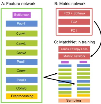
Figure 2.1: The MatchNet architecture. A: The feature network used for feature encoding, with an optional bottleneck layer to reduce feature dimension. B: The metric network used for feature comparison. C: In training, the feature net is applied as two “towers” on pairs of patches with shared parameters. Output from the two towers are concatenated as the metric network’s input. The entire network is jointly trained on labeled patch-pairs generated from the sampler to minimize the cross-entropy loss. In prediction, the two sub-networks (A and B) are conveniently used in a two-stage pipeline (See Section 2.5.2).
in filter supports and layer complexity compared to (Zbontar & LeCun, 2014). We evaluate architectural variations in Section 2.6.1.
2.4 Deep Neural Network Architecture
MatchNet is a deep-network architecture (Fig. 2.1 C) for jointly learning a feature network that maps a patch to a feature representation (Fig. 2.1 A) and a metric network that maps pairs of features to a similarity (Fig. 2.1 B). It consists of several types of layers commonly used in deep-networks for computer vision. We show details of these layer in Table 2.1, and discuss some of the high-level architectural choices in this section.
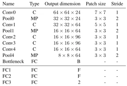
Table 2.1: Layer specification of MatchNet. The output dimension is given by (height × width×
depth). Patch size: patch size for convolution and pooling layers; Layer types: C: convolution, MP: max-pooling, FC: fully-connected. We always pad the convolution and pooling layers so the output height and width are those of the input divided by the stride. For FC layers, their size B and F are chosen from: B ∈ {64,128,256,512},F ∈ {128,256,512,1024}. All convolution and FC layers use ReLU activation except for FC3, whose output is normalized with Softmax (Equation 2.2).
Name Type Output dimension Patch size Stride
Conv0 C 64×64×24 7×7 1
Pool0 MP 32×32×24 3×3 2
Conv1 C 32×32×64 5×5 1
Pool1 MP 16×16×64 3×3 2
Conv2 C 16×16×96 3×3 1
Conv3 C 16×16×96 3×3 1
Conv4 C 16×16×64 3×3 1
Pool4 MP 8×8×64 3×3 2
Bottleneck FC B -
-FC1 FC F -
-FC2 FC F -
-FC3 FC 2 -
-Local Response Normalization or Dropout. We use Rectfied Linear Units (ReLU) as non-linearity for the convolution layers.
The metric network: We model the similarity between features using three fully-connected layers with ReLU non-linearity. FC3 also uses Softmax. Input to the network is the concatenation of a pair of features. We output two values in[0,1]from the two units of FC3, These are non-negative, sum up to one, and can be interpreted as the network’s estimate of probability that the two patches match and do not match, respectively.
Two-tower structure with tied parameters:The patch-based matching task usually assumes that patches go through the same feature encoding before computing a similarity. Therefore we need just one feature network. During training, this can be realized by employing two feature networks (or “towers”) that connect to a comparison network, with the constraint that the two towers share the same parameters. Updates for either tower will be applied to the shared coefficients.
max-pooling layers to deal with scale changes that are not present in stereo reconstruction problems, and it also has more convolutional layers compared to (Zbontar & LeCun, 2014).
In other settings, where similarity is defined over patches from two significantly different domains, the MatchNet framework can be generalized to have two towers that share fewer layers or towers with different structures.
The bottleneck layer: The bottleneck layer can be used to reduce the dimension of the feature representation and to control overfitting of the network. It is a fully-connected layer of sizeB, between the 4096 (8×8×64) nodes in the output of Pool4 and the final output of the feature network. We evaluate howBaffects matching performance in Section 2.6.1 and plot results in Figure 2.5.
The preprocessing layer: Following a previous convention, for each pixel in the input grayscale patch we normalize its intensity valuex(in[0,255]) to(x−128)/160. The resulting range of the input pixels is thus[−0.8,0.8].
2.5 Algorithms for Learning and Prediction
The feature and metric networks are trained jointly in a supervised setting using a two-tower structure illustrated in Figure 2.1-C. We minimize the cross-entropy error,
E =−1
n n X
i=1
[yilog( ˆyi) + (1−yi) log(1−yiˆ)], (2.1)
over a training set ofnpatch pairs using stochastic gradient descent (SGD) with a batch size of 32. Here
yiis the 0/1 label for input pairxi. 1 indicates match.yiˆ and1−yiˆ are the Softmax activations computed on the values of the two nodes in FC3,v0(xi)andv1(xi)as follows.
ˆ
yi =
ev1(xi)
ev0(xi)+ev1(xi). (2.2)
ˆ
yiis used as the probability estimate for label 1 in Equation 2.1.
Figure 2.2: All 24 of the 7×7filters learned in Conv0 from the liberty dataset. The pseudo-colors represent intensity.
Figure 2.2 visualizes Conv0 filters MatchNet learned on the Liberty dataset. Figure 2.3 visualizes the network’s response to an example patch at different layers in the feature network.
P
ool0
act
ivat
io
ns
P
ool1
act
ivat
io
ns
Conv
2
act
iv
at
ions
Conv
3
act
iv
at
ions
Conv
4
act
iv
at
ions
Input
pat
ch
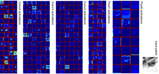
Figure 2.3: Visualization for the activations in response to an example input patch at different layers in the feature network. The input64×64patch is shown on the right. As sub-plot goes from right to left, we move up in the feature hierarchy. For each layer, we tile itsK H×W activation maps to form a 2D image.H,W andKare the height, width and depth of the 3D activation array respectively. Red margins separates these tiles. Pseudo-colors in the tiles represent response intensity. Although border artifacts can occur, we keep our padding scheme, for it retains half of the information on the original border.
2.5 Reservoir Sampling for Label Balancing
mini-Algorithm 2.1Generate a mini batch of size 2S with balanced pairs using a reservoir sampler. forb= 0. . . S−1do
Extract all patchesp1. . . pkfrom the next group;
Randomly choosepiandpj,i6=j,i, j∈ {1. . . k}; Samples(2b)←(1, pi, pj);
form= 0. . . kdo
Consider addingpm to the reservoir;1
end for
repeatat most 1000 times
Randomly drawpuandpvfrom the reservoir;
untilpuandpv are from different group;2 ifnegative sampling is successfulthen
Samples(2b+ 1)←(0, pu, pv);
else
Samples(2b+ 1)←(1, pi, pj);
end if end for
returnSamples;
batch so that the network will not be overly biased towards negative decisions. The sampler also enforces variety to prevent overfitting to a limited negative set.
Particularly, in our setting, the training set has already been grouped into matching patches; e.g. The UBC patch dataset has an average group size around 3. The learner streams through the training set by reading one group at a time. For positive sampling, we randomly pick two from the group; for negative sampling, we use a reservoir sampler (Vitter, 1985) with a buffer size ofRpatches. At any time
T the buffer maintainsRpatches as if uniformly sampled from the patch stream up toT, allowing a variety of non-matching pairs to be generated efficiently. The buffer size controls the trade-off between memory and negative variety. In our experiments,R= 128was too small and led to severe overfitting;
R= 16384has worked consistently. This procedure is detailed in Algorithm 2.1.
For instance, if the batch size is 32, in each training iteration we feed SGD 16 positives and 16 negatives. The positives are obtained by reading the next 16 groups from the database and randomly picking one pair in each group. Since we go through the whole dataset many times, even though we only pick one positive pair from each group in each pass, the network still gets good positive coverage,
1
Following (Vitter, 1985), if the sampler’s reservoir is not full, the candidate is always added; otherwise for the T-th candidate,
with probability R/T it is added and replaces a random element in the reservoir and with probability 1-R/T it gets rejected. R is
the reservoir size.
...
... ...
...
Patch set 1 Patch set 2
Feature set 1
Feature set 2
n1
n2
Pairwise matching scores Trained feature network
Trained metric network 64
64
B
B
n1 n2
n1
n2
n1 x n2
Feature pairs
2B
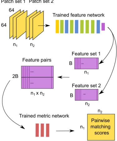
Figure 2.4: A Two-Stage prediction pipeline for computing pairwise matching score. MatchNet is disassembled during prediction. The feature network and the metric network run in a pipeline.
especially when the average group size is small. The 16 negatives are obtained by sampling two pairs from different groups from the reservoir buffer that stores previous loaded patches. At the first few iterations, the buffer would be empty or contain only matching patches. In that case we simply fill the slot in the batch with the most recent positive pair.
2.5 A Two-Stage Prediction Pipeline
A common scenario for patch-based matching is that there are sets of patches each extracted from two images. The goal is to compute aN1×N2matrix of pairwise matching scores, whereN1andN2are
experiment, on one NVIDIA K40 GPU, after tuning batch size, the feature net without bottleneck runs at 3.56K patch/sec; the metric net (B=128, F=512) runs at 416.6K pair/sec. The computation can be further pipelined and distributed for large-scale applications.
2.6 Evaluation on Image Patch Matching
2.6 Dataset and Evaluation Protocol
The UBC patch dataset (UBC)6was collected by Winder et al. (Winder et al., 2009) for learning descriptors. The patches were extracted around real interest points from several internet photo collections published in (Snavely et al., 2008). The dataset includes three subsets with a total of more than 1.5 million patches. It is suitable for discriminative descriptor or metric learning, and has been used as a standard benchmark dataset by many (Brown et al., 2011; Jia & Darrell, 2011; Trzcinski et al., 2012, 2013; Simonyan et al., 2014). The dataset comes with patches extracted using either Difference of Gaussian (DoG) interest point detector or multi-scale Harris corner detector. We use the DoG set.
There are three subsets in UBC: Liberty, Notredame and Yosemite. Each comes with pre-generated labeled pairs of 100k, 200k and 500k, all with 50% matches. Each also provides all unique patches and their corresponding 3D point ID. The number of unique patches in each dataset is 450k for Liberty, 468k for Notredame and 634k for Yosemite.
Following the standard protocol established in (Brown et al., 2011), people train the descriptor on one subset and test on the other two subsets. Although people may use any of the pre-generated pair sets or the grouped patches in the training subset for training and validation, the testing is done on the 100k labeled pairs in the test subset. The commonly used evaluation metric is the false positive rate at 95% recall (Error@95%), the lower the better.
2.6 Baseline Experiments with SIFT features
We use VLFeat (Vedaldi & Fulkerson, 2010)’svlsift()with default parameters and custom frame input to extract SIFT descriptor on patches. The frame center is the center of the patch at (32.5, 32.5). The scale is set to be 16/3, where 3 is the default magnifying coefficient, so that the bin size for the descriptor will be 16. With 4 bins along each side, the descriptor footprint covers the entire
6
patch. In our preliminary experiments we found that normalized SIFT (nSIFT), which is raw SIFT scaled so its L2-norm is 1, gives slightly better performance than SIFT, so nSIFT is used for all our baseline experiments.
For a pair of nSIFT, we compute similarity using L2, linear SVM on 128d element-wise squared difference features (Squared diff.) and a two-layer fully-connected neural networks on 256d nSIFT concatenation (Concat.). For nSIFT Square diff.+ linearSVM, we use Liblinear (Fan et al., 2008) to train the SVM and search the regularization parameter C among{10−4,10−3. . . ,104}using 10% of the
training set for validation. For nSIFT Concat.+ NNet, the network has the same structure (with F=512) as the metric network in MatchNet (Figure 2.1-B) and is trained using plain SGD with learning rate=0.01, batch size=128 and iteration=150k.
2.6 Variations of MatchNet
We evaluate MatchNet under different architectural variation. We train MatchNet using techniques described in Section 2.5 and evaluate the performance under different(F, B)combinations, whereF
andB are the dimension of fully-connected layers (F1 and F2) and the bottleneck layer respectively.
F ∈ {128,256,512,1024}. B ∈ {64,128,256,512}. We also evaluate using the feature network without the bottleneck layer.
We also evaluate MatchNet with feature quantization. The output features of the bottleneck layer in the feature tower (Figure 2.1-A) are represented as floating point numbers. They are the outputs of ReLu units, thus the values are always non-negative. We quantize these feature values in a simplistic way. For a trained network, we compute the maximum valueMfor the features across all dimensions on a set of random patches in the training set. Then each elementv in the feature is quantized as
q(v) = min(2n−1,b(2n−1)v/Mc), wherenis the number of bits we quantize the feature to. When the feature is fed to the metric network,vis restored usingq(v)M/(2n−1). We evaluate the performance using different quantization levels.
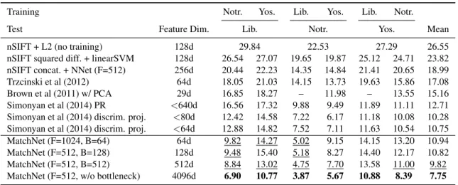
Table 2.2: Patch matching results on UBC dataset. Numbers are Error@95% in percentage. See Section 2.6.1 for descriptions of different settings. F and B are dimensions for fully-connected and bottleneck layers in Table 2.1. Boldnumbers are the best results across all conditions. Underlined numbers are better than the previous state-of-the-art results with similar feature dimension.
Training Notr. Yos. Lib. Yos. Lib. Notr.
Test Feature Dim. Lib. Notr. Yos. Mean
nSIFT + L2 (no training) 128d 29.84 22.53 27.29 26.55
nSIFT squared diff. + linearSVM 128d 26.54 27.07 19.65 19.87 25.12 24.71 23.82
nSIFT concat. + NNet (F=512) 256d 20.44 22.23 14.35 14.84 21.41 20.65 18.99
Trzcinski et al (2012) 64d 18.05 21.03 14.15 13.73 19.63 15.86 17.08
Brown et al (2011) w/ PCA 29d 16.85 18.27 – 11.98 – 13.55 15.16
Simonyan et al (2014) PR <640d 16.56 17.32 9.88 9.49 11.89 11.11 12.71
Simonyan et al (2014) discrim. proj. <80d 12.42 14.58 7.22 6.17 11.18 10.08 10.28 Simonyan et al (2014) discrim. proj. <64d 12.88 14.82 7.52 7.11 11.63 10.54 10.75
MatchNet (F=1024, B=64) 64d 9.82 14.27 5.02 9.15 14.15 13.20 10.94
MatchNet (F=512, B=128) 128d 9.48 15.40 5.18 8.27 14.40 12.17 10.82
MatchNet (F=512, B=512) 512d 8.84 13.02 4.75 7.70 13.58 11.00 9.82
MatchNet (F=512, w/o bottleneck) 4096d 6.90 10.77 3.87 5.67 10.88 8.39 7.75
1024bits. Of course, employing a more sophisticated encoding mechanism should further improve compactness.
2.6 Results and Discussion
We follow the evaluation protocol and evaluate MatchNet along with several SIFT baselines and other learned float descriptors. Results for SIFT baselines and MatchNet with floating point features are listed in Table 2.2. Our best model 4096-512x512 (feature dim.-FxF) achieves best performance over all evaluation pairs. It achieves7.75%average error rate vs. (Simonyan et al., 2014)’s<80f at 10.38%. With a bottleneck of 64d, our 64-1024×1024 model achieves 10.94% average error rate vs. (Simonyan et al., 2014)’s 10.75% using features with about the same dimension.
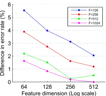
One advantage of our approach is that we can easily vary feature dimension and matching complexity and jointly optimize them. The trade off between storage/computation vs. accuracy is plotted in Figure 2.5. Not suprisingly, increasing F and B leads to lower error rate, but the absolute gain is diminishing exponentially.
64
128
256
512
0
1
2
3
4
5
6
Feature dimension (Log scale)
Difference in error rate (%)
F=128 F=256 F=512 F=1024
Figure 2.5: Accuracy vs. dimensionality tradeoff for different fully-connected layer sizes. we plot the average difference in Error@95% between other(F, B)combinations and(F = 1024, B= 512)across all 6 train-test pairs in UBC. Features are unquantized.
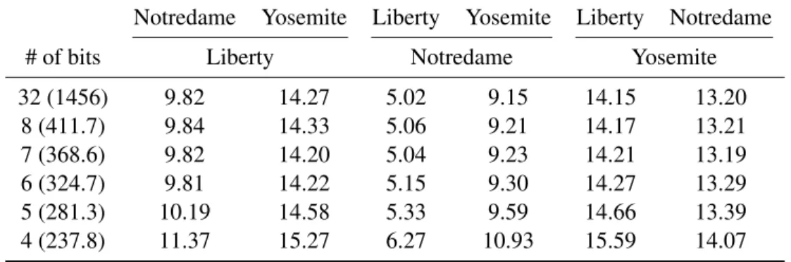
representation while using only 325 bits instead of 1024. For 6-bit quantization, the feature has324.7 bits (40.6bytes) per patch on average. Our results also show that going from a 32-bit floating point representation to a 6-bit one yields little degradation in performance. We attribute this to the robustness of the matching network.
Our baseline experiments with SIFT features confirms that a better metric can significantly improve performance. For instance, in Yosemite-Liberty, nSIFT concat.+NNet performs better than nSIFT+L2 by 7.61% in absolute error rate, and MatchNet with the same feature dimension (128) and fully-connected layer dimension (512) achieves a further improvement of 6.7% in absolute error rate. The benefit of coupling the descriptor and the metric has been explored in different forms in the past. For instance, (Simonyan et al., 2014) learns weights for each pooling regions, so does (Trzcinski et al., 2012) for each weak gradient map learner to form a Mahalanobis type of similarity. Our proposed unification through neural networks is a simple and powerful alternative.
Table 2.3: Accuracy vs. quantization tradeoff for the 64-1024×1024 network. Names in the first row and second row are names of the training set and test set respectively. In the first column, the first value is bits per dimension. The second value is average bits per feature vector. It is computed using 64 + 64×0.679×b, where b is the number of bits per dimension, and the average density (non-zeros) of the feature vector is 67.9%. Numbers in the middle are Error@95%. The first row is for the un-quantized features.
Notredame Yosemite Liberty Yosemite Liberty Notredame
# of bits Liberty Notredame Yosemite
32 (1456) 9.82 14.27 5.02 9.15 14.15 13.20
8 (411.7) 9.84 14.33 5.06 9.21 14.17 13.21
7 (368.6) 9.82 14.20 5.04 9.23 14.21 13.19
6 (324.7) 9.81 14.22 5.15 9.30 14.27 13.29
5 (281.3) 10.19 14.58 5.33 9.59 14.66 13.39
4 (237.8) 11.37 15.27 6.27 10.93 15.59 14.07
be enough to explain our∼3% absolute gain for Liberty-Notredame. On one hand, the top curve in (Simonyan et al., 2014)’s Fig. 3 shows a diminishing gain. Without discriminative projection, at around 1500d, the error rate is still above 9%, more than twice as much as MatchNet’s error rate (3.87%) with 4096d patch representation. On the other, with a 512d bottleneck and quantization, MatchNet still outperforms (Simonyan et al., 2014)’s PR (<640d) results in 4 out of 6 train-test pairs with up to 7% improvement in absolute error rate.
Supported by the tradeoff results in Figure 2.5 and Table 2.3, we provide the following guidelines to enable users to choose a configuration based on their storage/computation constraints: The 4096-512x512 model should be used if the feature dimension is not a concern, or if accuracy takes priority. This model outperforms others by a large margin on UBC. If extra compression is needed, the 64-1024x1024 one with quantization should be used.
2.7 Cross-domain Similarity for Exact-Match Clothing Item Retrieval
2.7 Exact Street to Shop
In this section, we discuss how to apply similarity learning to a challenging clothing item retrieval problem, which we call “Exact Street to Shop”. Given a real-world photo of a clothing item, e.g. taken on the street, the goal of this task is to find that clothing item in an online shop. This is extremely challenging due to differences between depictions of clothing in real-world settings versus the clean simplicity of online shopping images. For example, clothing will be worn on a person in street photos, whereas in online shops, clothing items may also be portrayed in isolation or on mannequins. Shop images are professionally photographed, with cleaner backgrounds, better lighting, and more distinctive poses than may be found in real-world, consumer-captured photos of garments. To deal with these challenges, we introduce a deep learning based methodology to learn a similarity measure between street and shop photos.
The street-to-shop problem has been recently explored (Liu et al., 2012). Previously, the goal was to find similar clothing items in online shops, where performance is measured according to how well retrieved images match a fixed set of attributes, e.g. color, length, material, that have been hand-labeled on the query clothing items. However, finding a similar garment item may not always correspond to what a shopper desires. Often when a shopper wants to find an item online, they want to findexactlythat item to purchase. Therefore, we define a new task,Exact Street to Shop, where our goal is for a query street garment item, to find exactly the same garment in online shopping images.
2.7 Item Localization
listed under the correct category and shoppers can always locate the item of interest, which means the shops have no motivation to annotate the exact location of items. Therefore, the distinction of computing similarity at image-level and item-level affects how we process the shop images. We show in Section 2.8 that using item-level similarity significantly improves the retrieval success rate. Therefore localization matters.
Since clothing parsing is still an ongoing research (Yamaguchi et al., 2013), we cannot simply rely on a clothing parser to get bounding boxes for items in shop images. Instead, we use the selective search method (van de Sande et al., 2011), a high-recall, automatic, generic object proposal method to generate multiple candidate bounding boxes. This method is expected to output boxes that contain the clothing item or contain part of them, while rejecting a large number of boxes that contains only the background. The idea is that we improve the localization of the item of interest at the cost of more comparison.
More specifically, we use the selective search algorithm and filter out proposals with a width smaller than 15 of the image width since these usually correspond to false positive proposals. From this set, the 100 most confident object proposals are kept. This remaining set of object proposals has an average recall of 97.76%, evaluated on an annotated subset of 13,004 shop item photos.
2.7 Similarity Learning
For similarity, our hypothesis is that the cosine similarity on existing convolutional neural network (CNN) features may be too general to capture the underlying differences between the street domain and the shop domains. Therefore, we explore methods to learn a data-driven similarity.
Inspired by recent work on deep similarity learning for matching image patches between images of the same scene (Han et al., 2015; Zagoruyko & Komodakis, 2015; Zbontar & LeCun, 2015), we model the similarity between a query feature descriptor and a shop feature descriptor with a three-layer fully-connected network and learn the similarity parameters for this architecture. Here, labeled data for training consists of positive samples, selected from exact street-to-shop pairs, and negative samples, selected from non-matching street-to-shop items.
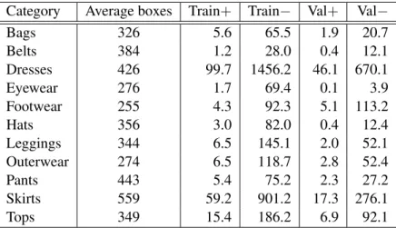
Category Average boxes Train+ Train− Val+ Val−
Bags 326 5.6 65.5 1.9 20.7
Belts 384 1.2 28.0 0.4 12.1
Dresses 426 99.7 1456.2 46.1 670.1
Eyewear 276 1.7 69.4 0.1 3.9
Footwear 255 4.3 92.3 5.1 113.2
Hats 356 3.0 82.0 0.4 12.4
Leggings 344 6.5 145.1 2.0 52.1
Outerwear 274 6.5 118.7 2.8 52.4
Pants 443 5.4 75.2 2.3 27.2
Skirts 559 59.2 901.2 17.3 276.1
Tops 349 15.4 186.2 6.9 92.1
Table 2.4: Size statistics of the training and validation sets for similarity learning. Average boxes shows the number of selective search boxes used, averaged across query images with at least one successful retrieval within the short list. Numbers in the last four columns are in units of 1,000.
or “do not match”, which is consistent with the use of cross-entropy loss during training. Once we have trained our network, during the test phase, we use the “match” output prediction as our similarity score. Previous work has shown that this type of metric network has the capacity for approximating the underlying non-linear similarity between features. For example, Han et al. (Han et al., 2015) showed that the learned similarity for SIFT features, modeled by such a network, is more effective than L2-distance or cosine-similarity for matching patches across images of a scene.
We formulate the similarity learning task as a binary classification problem, in which positive/negative examples are pairs of CNN features from a query bounding box and a shop image selective-search based item proposal, for the same item/different items. We minimize the cross-entropy error
E=−1
n n X
i=1
[yilog( ˆyi) + (1−yi) log(1−yiˆ)] (2.3)
over a training set ofnbounding box pairs using mini-batch stochastic gradient descent. Here,yi= 1
for positive examples;yi= 0for negative examples; andyˆiand1−yˆi are the two outputs of the metric
Dresses
Outerwear Pants
Skirts Tops
Dress metric net
Train a category-independent metric network
Finetune with pairs from each category
Multiple category-specific networks
Outerwear metric net
...
Hats metric netFully-connected Fully-connected Regression
Shop Street
Matching score
Figure 2.6: Illustration of the training, followed by fine-tuning procedure for training category-specific similarity for each category. To deal with limited data, we first train a generic similarity using five large categories and then fine-tune it for each category individually. See Section 2.7.3 for more description. item, some images on the shop side will bear little similarity in appearance to a particular query item view. Labeling such visually distinct pairs as positives would likely confuse the classifier during training.
We handle these challenges by training our metric network on a short list of top retrieved shop bounding boxes using the object proposal retrieval approach described above. At test time, we perform the same primitive retrieval to obtain a short list of candidate retrievals and then re-rank the list using our learned similarity. This has an added benefit of improving the efficiency of our retrieval approach since the original cosine similarity measure is faster to compute than the learned similarity. Moreover, for real application, the entire primitive retrieval could be implemented efficiently using a proper binary hashing mechanism such as muilt-index hashing (Norouzi et al., 2014).
More specifically, to construct training and validation sets for similarity learning, for each training query item,q, we retrieve the top 1000 selective search boxes from shop images using cosine similarity. For each bounding boxbfrom a shop image in this set,(q, b)is a positive sample if the shop image is a street-to-shop pair withq. Otherwise,(q, b)is used as a negative sample7.
We randomly split the queries intotrainandvalsets in a 2:1 ratio. such thatvalcontains half the number of items as the test set. Statistics fortrainandvalare shown in Table 2.4 for our retrieval experiments.
7
Intuitively, we might want to train a different similarity measure for each garment category, for example, objects such as hats might undergo different deformations and transformations than objects like dresses. However, we are limited in the number of positive training examples for each category and by the large negative-to-positive ratio. Therefore, we employ negative sampling to balance the positive and negative examples in each mini-batch. We train a general street-to-shop similarity measure, followed by fine-tuning for each garment category to achievecategory-specificsimilarity (See Figure 2.6).
In the first stage of training, we select five large categories from our garment categories: Dresses, Outerwear, Pants, Skirts, and Tops and combine their training examples. Using these examples, we train an initialcategory-independentmetric network. We set the learning rate to 0.001, momentum to 0.9, and train for 24,000 iterations, then lower the learning rate to 0.0001 and train for another 18,000 iterations. In the second stage of learning, we fine-tune the learned metric network on each category independently (with learning rate 0.0001), to produce category-dependent similarity measures. In both stages of learning, the corresponding validation sets are used for monitoring purposes to determine when to stop training.
2.8 Evaluation on Exact-Match Clothing Item Retrieval
2.8 Dataset and Evaluation Protocol
TheExact Street2Shop Dataset8is collected by M. Hadi Kiapour (Kiapour et al., 2015). It contains street photos, shop photos and street-to-shop correspondences in 11 garment categories: Bags, Belts, Dresses, Eyewear, Footwear, Hats, Leggings, Outerwear, Pants, Skirts and Tops. Street photos are amateur fashion photographs of people wearing clothing items. Shop photos are professional photographs listed in online shopping websites representing a specific clothing item. On the shop side, a clothing item is usually represented in multiple shots including but not limited to a frontal shot, a back shot and a close-up shot. Examples of the street photos and shop photos can be seen in Figure 2.7.
8
Figure 2.7: Example of street photos (the six ones on the left) and shop photos (the six ones on the right).
Street-to-shop correspondences are collected from the style galleries of ModCloth website9. These style galleries contain user-uploaded posts with street photos as well links to the shopping page on ModCloth where items in the photos can be purchased. Figure 2.8 shows a screenshot of an example post in the gallery, where the street-to-shop correspondence occurs.
The dataset also includes bounding boxes over items with corresponding shop photos and shop images from 24 other online stores, such as TheRealReal, Amazon, NordStrom, etc.
For experiments that involves learning, we split the exact matching pairs into two disjoint sets such that there is no overlap of items in street and shop photos between train and test. In particular, for each category, the street-to-shop pairs are distributed into train and test splits with a ratio of approximately 4:1. For our retrieval experiments, a query consists of two parts: 1) a street photo with an annotated bounding box indicating the target item, and 2) the category label of the target item. We view these as simple annotations that a motivated user could easily provide, but this could be generalized to use automatic detection methods. Since the category is assumed to be known, retrieval experiments are performed within-category. Street images may contain multiple clothing items for retrieval. We consider each instance as a separate query.
Performance is measured in terms oftop-kaccuracy, the percentage of queries with at least one matching item retrieved within the firstkresults.
2.8 Main Results
Following the above protocol, we compare across all categories four different similarity models: Cosine similarity on whole image (Whole Image), Cosine similarity on selective search boxes (Selec-tive Search), Learned category-independent similarity on selec(Selec-tive search boxes (Similarity), Learned category-specific similarity (F.T. Similarity). We use pre-trained AlexNet (Krizhevsky et al., 2012) FC6 activations as feature representation across all four models.
Table 2.5 (right) presents the exact matching performance of our baselines and learned similarity approaches (before and after fine-tuning) fork=20. Whole image retrieval performs the worst on all categories. The object proposal method improves over whole image retrieval on all categories, especially on categories like eyewear, hats, and skirts, where localization in the shop images is quite useful. Skirts,
Category Queries Query Items Shop Images Shop Items Whole Im. Sel. Search Sim. F.T. Sim.
Bags 174 87 16,308 10,963 23.6 32.2 31.6 37.4
Belts 89 16 1,252 965 6.7 6.7 11.2 13.5
Dresses 3,292 1,112 169,733 67,606 22.2 25.5 36.7 37.1
Eyewear 138 15 1,595 1,284 10.1 42.0 27.5 35.5
Footwear 2,178 516 75,836 47,127 5.9 6.9 7.7 9.6
Hats 86 31 2,551 1,785 11.6 36.0 24.4 38.4
Leggings 517 94 8,219 4,160 14.5 17.2 15.9 22.1
Outerwear 666 168 34,695 17,878 9.3 13.8 18.9 21.0
Pants 130 42 7,640 5,669 14.6 21.5 28.5 29.2
Skirts 604 142 18,281 8,412 11.6 45.9 54.6 54.6
Tops 763 364 68,418 38,946 14.4 27.4 36.6 38.1
Table 2.5: Test dataset statistics and top-20 item retrieval accuracy for the Exact-Street-to-Shop task. The last four columns report performance using whole-image features, selective search bounding boxes, and re-ranking with learned generic similarity or fine-tuned similarity.
for example, are often depicted on models or mannequins, making localization necessary for accurate item matching. We also trained category-specific detectors (Girshick et al., 2014) to remove the noisy object proposals from shop images. Keeping the top 20 confident detections per image, we observe a small drop of 2.16% in top-20 item accuracy, while we are able to make the retrieval runtime up to almost an order of magnitude more efficient (e.g. 7.6x faster for a single skirt query on one core).
Our final learned similarity after category-specific fine-tuning achieves the best performance on almost all categories. The one exception is eyewear, for which the object proposal method achieves the best top-20 accuracy. The initial learned similarity measure before fine-tuning achieves improved performance on categories that it was trained on, but less improvement on the other categories.
✔
✔
✔
Figure 2.9: Example retrievals using category-specific similarity. Top and bottom three rows show example successful and failure cases respectively.
Figure 2.10: Top-kitem retrieval accuracy for different numbers of retrieved items.
the performance of our similarity network grows significantly faster than the baseline methods. This is particularly useful for real-world search applications, where users rarely look beyond the first few highly ranked results.
2.9 Summary
We propose and evaluate a unified approach for patch-based image matching that jointly learns a deep convolutional neural network for local patch representation as well as a network for robust feature comparison. Our system trains models that achieve state-of-the-art performance on a standard dataset for patch matching. We also evaluate a suite of architectural variations to study the tradeoff between accuracy vs. storage/computation. This work demonstrates that deep convolutional neural networks can be effective for general wide-baseline patch matching. In addition, an important feature of these results is that MatchNet can produce state-of-the-art accuracies while using significantly fewer bits per feature even than very recent work on compact feature representations, even with very simple quantization. This suggests that using deep learning approaches—and more advanced quantization—can make even more significant improvements in the accuracy/feature size trade-off.
CHAPTER 3
MULTIPLE-VOXEL PATTERN CLASSIFIER LEARNING FOR FMRI IMAGES10 3.1 Introduction
Studies of human and nonhuman primates have consistently shown that the ventral temporal and occipital regions are involved in the perception and recognition of visual stimuli (see review by Ungerlei-der & Haxby (1994)). These visual association regions in the posterior cortex show functional divisions specializing in categorical representation of objects such as faces, tools, words, etc. (e.g., Epstein & Kanwisher (1998); Chao et al. (1999)). It has been proposed that these regions are also involved in supporting visual working memory the short-term representation of visual stimuli that are no longer physically available (Postle, 2006; Ranganath & D’Esposito, 2005). Neuroimaging findings, however, have been inconsistent thus far. Some showed that the inferior temporal region (e.g., lateral fusiform gyrus) was active in tasks requiring holding faces (e.g., Druzgal & D’esposito (2003); Postle et al. (2003); Ranganath et al. (2004)) and in tasks requiring refreshing recently seen faces (e.g., Johnson et al. (2007)). Others, however, showed that the activity in the inferior temporal region was not long lasting (Jha & McCarthy, 2000) and subject to interference (Miller et al. (1993); Sreenivasan et al. (2007), but see Yoon et al. (2006) for different results).
Some investigators further examined the selectivity of the posterior visual association regions in representing specific visual working memory. Face and/or scene images were used as task stimuli in neuroimaging studies since the fusiform (FG) and parahippocampal gyri (PHG) are known to be more specialized in processing faces and scenes, respectively (e.g., Kanwisher et al. (1997); Epstein & Kanwisher (1998)). Participants were cued to remember a particular category of visual stimuli (e.g., Remember face but ignore scene, and vice versa), with the cue presented either prior to stimulus presentation for selective encoding (Gazzaley et al., 2005; Nobre et al., 2004) or after, for selective maintenance (Oh & Leung, 2010; Lepsien et al., 2005). Across studies, the PHG consistently showed elevated activity during selective encoding and selective maintenance of scene images. The FG, however,
10