IMPROVEMENTS IN MASS SPECTROMETRIC ANALYSES WITH
DIFFERENTIAL ION MOBILITY SPECTROMETRY
Samantha L. Isenberg
A dissertation submitted to the faculty of the University of North Carolina at Chapel hill in partial fulfillment of the requirements for the degree of Doctor of Philosophy in the
Department of Chemistry
Chapel Hill 2014
Approved by:
Gary L. Glish
ii © 2014
iii ABSTRACT
Samantha L. Isenberg: Improvements in Mass Spectrometric Analyses with Differential Ion Mobility Spectrometry
(Under the direction of Gary L. Glish)
Mass spectrometry (MS) based analyses of complex samples often require separations to improve signal-to-background and remove isobaric and isomeric interferences prior to mass analysis. Chromatographic and electrophoretic separations are commonly employed prior to ionization, but these separations can add minutes to hours to mass spectrometric analyses. Ion mobility spectrometry (IMS) has the ability to separate ions based on shape-to-charge rather than mass-to-shape-to-charge, making IMS complementary to MS. IMS has been shown to improve signal-to-background and have the ability to separate isomeric/isobaric species.
iv
v
ACKNOWLEDGEMENTS
First and foremost, I would like to thank Dr. Gary Glish for guidance, support and patience over the years. Thank you for the freedom you have given me in conducting my own research, allowing me to become an independent, confident scientist.
I am so blessed to have had my parents' unwavering support over the years. I truly cannot put into words how lucky I am.
vi
TABLE OF CONTENTS
LIST OF TABLES...x
LIST OF FIGURES...xii
LIST OF ABBREVTIATIONS AND SYMBOLS...xvi
CHAPTER 1: INTRODUCTION TO DIFFERENTIAL ION MOBILITY SPECTROMETRY...1
1.1 Separations with mass spectrometry...1
1.2 Introduction to ion mobility spectrometry...2
1.3 Differential ion mobility spectrometry...5
1.3.1 Background...5
1.3.2 Current uses...10
1.3.3 Issues/drawbacks of DIMS...10
1.4 Summary...11
1.5 REFERENCES...14
CHAPTER 2: EXPERIMENTAL...17
2.1 Materials...17
2.2 Mass spectrometry...17
2.3 Ion mobility spectrometry...19
2.3.1 Differential ion mobility spectrometry...19
2.3.2 Trapped ion mobility spectrometry...22
vii
2.5 REFERENCES...27
CHAPTER 3: OPTIMIZATION OF DIMS SEPARATIONS...28
3.1 Evaluation of DIMS separations...28
3.2 Electrode dimensions...29
3.2.1 Ion transmission with DIMS transparent...29
3.2.2 Ion transmission with active DIMS: generation 3...31
3.2.3 From generation 3 to generation 4: ion transmission and resolving power...36
3.3 Carrier gas parameters...37
3.3.1 Carrier gas temperature...37
3.3.2 Desolvation gas flow rate...39
3.4 Carrier gas composition: adding helium to the mix...41
3.4.1 Using helium to improve DIMS separations...41
3.4.2 Linked scanning...43
3.4.3 Maximum ED for varying %He...47
3.5 Separation of 3 isobaric peptides...49
3.6 Summary and conclusions...52
3.7 REFERENCES...54
CHAPTER 4: DIMS FOR THE INVESTIGATION OF ION REACTIONS IN TRANSFER OPTICS...55
4.1 Introduction to ion reactions in transfer optics...55
4.1.1 Ion transfer optics for ESI-MS...55
4.1.2 Ion reactions before, within, and after DIMS...56
viii
4.2.1 Ion reactions after DIMS can convolute results...58
4.2.2 Optimization of DIMS-MS analyses for fragile analytes...62
4.3 Charge reduction in transfer optics elucidated by DIMS...66
4.3.1 Evidence of a charge reduction after DIMS...66
4.3.2 Where does charge reduction occur?...67
4.3.3 Capillary functionalization...72
4.3.4 Collision cross-sections from TIMS...73
4.4 Summary and conclusions...75
4.5 REFERENCES...77
CHAPTER 5: DIMS AS AN ELECTRONIC IMMUNOASSAY...78
5.1 Biomarker detection and quantification...78
5.1.1 Current methods...78
5.1.2 Brain natriuretic peptide immunoassays...79
5.2 BNP in serum...80
5.3 Importance of peptide structure in DIMS separations...81
5.4 LOD of BNP in human plasma...85
5.5 Detection of Leukemia antigens...89
5.6 Summary and conclusions...93
5.7 REFERENCES...95
CHAPTER 6: DIMS FOR THE ANALYSIS OF AEROSOLS...97
6.1 Introduction to the analysis of aerosols...97
6.2 Experimental: pyrolysis...99
ix
6.3.1 Need for separations with aerosol analysis...100
6.3.2 Differential ion mobility spectrometry...102
6.3.3 Trapped ion mobility spectrometry...109
6.4 Summary and conclusions...114
6.5 REFERENCES...116
CHAPTER 7: SUNMMARY AND FUTURE WORK...118
7.1 General Summary...118
7.2 Optimization of DIMS separations...118
7.2.1 Summary...118
7.2.2 Future directions...119
7.3 Investigation of ion reactions using DIMS...121
7.3.1 Summary...121
7.3.2 Future directions...122
7.4 Detection of biomarkers in plasma...123
7.4.1 Summary...123
7.4.2 Future directions...125
7.5 Aerosol analysis...126
7.5.1 Summary...126
7.5.2 Future directions...127
7.6 REFERENCES...129
x
LIST OF TABLES
2.1 Chemical formulae for components in Agilent ESI tuning mix...18 2.2 Dimensions of DIMS electrodes...19 2.3 Reduced ion mobility and collision cross-sections in
nitrogen for components in Agilent ESI tuning mix used
for TIMS calibration...25 3.1 Ion transmission with DIMS transparent observed for
tetrabutyl ammonium ion (m/z 242), angiotensin 13+ (m/z 433)
and BNP5+ (m/z 694)...30 3.2 %T and RP obtained using BNP...37 3.3 RP for protonated YGGFL (m/z 556) for varying desolvation
gas temperatures at ED of 26, 30, and 34 kV/cm...39 3.4 RP for each peptide in mixture at 0, 20 and 40% He and for
the linked scan...45 3.5 RP for 7+ (1225), 8+ (m/z 1072), and 9+ (m/z 953) charge
states of ubiquitin at 0, 20 and 40% He and for the linked scan...47 3.6 Ion transmission, resolving power and resolution for each % helium...48 4.1 Average ratio of peak B to peak A for 18 cm and 30 cm
long capillaries...71 4.2 Ratios of peak B to peak A for regular and functionalized
capillaries...73 5.1 Dilution of FBS extract to minimize ionization suppression...80 5.2 Results of DIMS scans for angiotensin3+ with and without
the addition of DTT to the electrospray solvent...83 5.3 Results of DIMS scans for ANP4+ (native and reduced),
ratBNP6+ (native and reduced) and Gramacidin S2+
(linear and cyclic)...84 5.4 Results obtained from LOD curves with DIMS for BNP
xi
5.5 Results obtained from LOD curves obtained with CID
without and with DIMS for BNP in human plasma...88 5.6 Results obtained from LOD curves obtained with PTR
without and with DIMS for BNP in human plasma...88 6.1 Structures, relative energies for neutrals and theoretical
cross-section of the protonated molecules determined from proposed structures for the ion observed at m/z 111
xii
LIST OF FIGURES
1.1 Representation of IMS drift-tube...2
1.2 TWIMS cell operating as an ion guide in (a) and as an ion mobility spectrometer in (b)...4
1.3 Representation of the steps of a TIMS separation...5
1.4 Representation of ion mobility as a function of electric field for three ions...6
1.5 DIMS geometries with (a) cylindrical and (b) planar electrodes...7
1.6 Representation of DIMS operating in filter mode...8
2.1 Nomenclature used for peptide product ions...19
2.2 DIMS assemblies G3 and G4...20
2.3 Simplified representation of the addition of two sinusoidal waves to create the bisinusoidal waveform...21
2.4 TIMS assembly with entrance funnel, analyzer region, and exit funnel...23
2.5 Simplified representation of TIMS separations...23
2.6 Calibration plot used for TIMS experiments correlating reduced ion mobility to inverse voltage...25
3.1 Ions entering the gap between the electrodes at various positions and time points during a cycle of the asymmetric waveform...32
3.2. A simplified visualization of a constrained effective analytical gap...33
3.3. Ion transmission for DIMS active observed for angiotensin I with varying electrode dimensions...34
3.4. a) Ion transmission for DIMS active observed for the tetrabutyl ammonium ion (m/z 242) with varying electrode dimensions and b) RP with varying electrode dimensions...35
xiii
3.6 DIMS scans obtained as desolvation gas flow rate is varied
at a fixed ED of 72 kV/cm...40
3.7 Resolution of a mixture of isobaric peptides, YLFTLEPQT and LLSLLLLMPV (m/z 1112) with 20% and 50% He in N2 carrier gas...43
3.8 Separation of a peptide mixture with a) 0% He, b) 20% He, c) 40% He, and d) linked scan from 40 to 0% He...44
3.9 Peak observed for protonated YGGFL (m/z 556) for varying %He and for linked scan...46
3.10 CV scans of isobaric peptides...50
3.11 MS/MS spectra of a mixture of nominally isobaric peptides...51
4.1 Basic schematic of ESI-DIMS-MS instrument...56
4.2 Example DIMS-MS scan of a protonated molecule (MH+) and its fragment (F+) formed via ESI and in the transfer optics...57
4.3 DIMS analysis of protonated GGG...60
4.4 DIMS analysis of sodiated monosaccharides...62
4.5 MS of myoglobin observed using default ion optics settings and 100% water as the ESI solvent...63
4.6 DIMS scans (ED=30 kV/cm) of myoglobin...64
4.7 MS of myoglobin utilizing adjusted transfer optics settings to minimize fragmentation in ion optics (a) without DIMS, and (b) with DIMS active...65
4.8 DIMS scan of angiotensin I...66
4.9 DIMS scans of bradykinin, with varying dispersion fields...67
4.10 DIMS scans of bradykinin with varying capillary-to-skimmer offset...68
xiv
4.12 DIMS scans for bradykinin2+ with an 18 cm capillary and a
30 cm capillary...71
4.13 Functionalization of glass transfer capillary via reaction with trimethylchlorosilane...72
4.14 DIMS scans of bradykinin with regular capillary and functionalized capillary...73
4.15 TIMS scans with DIMS in filter mode for bradykinin...74
5.1 Brain natriuretic peptide (BNP)...79
5.2 DIMS spectra of BNP5+in FBS extract...81
5.3 Representative DIMS scans of native (a) and reduced (b) BNP5+...82
5.4 DIMS scans of ANP5+: native and reduced peptide...85
5.5 Mass spectra obtained for BNP in human plasma extract with and without DIMS...86
5.6 LOD curves for BNP in a human plasma extract...87
5.7 MS/MS of protonated FLSSANEHL (GLR) in peptide mix with and without DIMS...91
5.8 Sum of the intensities of the five most intense product ions observed from MS/MS of protonated FLSSANEHL as a function of the concentration of FLSSANEHL (GLR) in the mixture of 94 peptides with and without DIMS...92
5.9 (a) DIMS scan of sodiated FLLPTGAEA (m/z 940.6) and MS/MS obtained for sodiated FLLPTGAEA in a peptide cell extract with and without DIMS...93
6.1 Ambient ionization techniques used for aerosol analyses: (a) PyEESI (b) PyLTPI...100
6.2 Mass spectrum obtained from in-line PyLTPI of cellulose at 650°C...101
xv
6.4 Mass spectra obtained from PyLTPI of ethyl cellulose at 650°C
with (a) linear ion trap and (b) FTICR...104 6.5 MS/MS of the ion observed at m/z 199 from the PyLTPI
of ethyl cellulose with labeled chemical formulae...105 6.6 DIMS results for the ion observed at m/z 199 from PyLTPI
of ethyl cellulose...106 6.7 DIMS results for the ion observed at m/z 163 from the PyEESI
of cellulose...107 6.8 DIMS results for the ion observed at m/z 183 from the PyLTPI of
(a) ethyl cellulose at 40 kV/cm (b) ethyl cellulose spiked with syringaldehyde, and MS/MS spectra obtained (c) without being spiked with syringaldehyde and (d) selecting for spiked
syringaldehyde with DIMS...108 6.9 TIMS scan for PyLTPI of cellulose at 650°C where mass-to-charge
ratio is plotted as a function of mobility spectrum number...109 6.10 TIMS spectra for isobars observed at m/z 163...110 6.11 Relative intensity of the ion observed at m/z 111 from PyLTPI
xvi
LIST OF ABBREVIATIONS AND SYMBOLS
A alanine
Å Angstrom (10-10 meters)
ANP atrial natriuretic peptide BNP brain natriuretic peptide
C cysteine
CCS collision cross-section
CG1 antigen peptide FLLPTGAEA
CID collision-induced dissociation
cm centimeter
CPC condensation particle counter
CV compensation voltage
Cys cysteine
°C degrees Celsuis
D diffusion
D aspartic acid
Da dalton
dc direct current
Δd oscillation amplitude of ion in DIMS during one period of the waveform (dh-dl)
DFT density functional theory
dh displacement of ion during high field portion of waveform
DIMS differential ion mobility spectrometry
xvii
DIMS-MS/MS differential ion mobility spectrometry coupled to tandem mass spectrometry
dl displacement of ion during low field portion of waveform
DMA differential mobility analyzer DTIMS drift-tube ion mobility spectrometry
DTT dithiothreitol
DV dispersion voltage
E electric field
E glutamic acid
e fundamental charge constant (1.602 × 10⁻¹⁹ coulombs/mole) EC compensation field (compensation voltage divided by gap between
electrodes)
ED dispersion field (dispersion voltage divided by gap between electrodes)
EESI extractive electrospray ionization El low electric field (< ~104 V/cm)
Eh high electric field (> ~104 V/cm)
EI electron ionization
ESI electrospray ionization
F phenylalanine
f frequency
F+ fragment ion
FBS fetal bovine serum
Fmoc 9-fluorenylmethoxycarbonyl
xviii
FWHM full-width at half-max of a Gaussian peak
G glycine
g gap between electrodes
G3 generation 3
G4 generation 4
GC gas chromatography
GC-DIMS gas chromatography coupled to differential ion mobility spectrometry ge effective analytical gap (g-Δd)
GLR antigen peptide FLSSANEHL
H histidine
HCT high capacity trap
He helium
HLA human leukocyte antigen
HPLC high-performance liquid chromatography
Hz Hertz
%He percent helium
I isoleucine
ICP inductively coupled plasma
i.d. inner diameter
IMS ion mobility spectrometry
IMS-MS ion mobility spectrometry coupled to mass spectrometry K ion mobility (cm2V-1s-1)
xix
K0 reduced ion mobility
kB Boltzmann's constant (1.38 × 10⁻²³ J/K)
kHz kiloHertz (103 Hertz)
Kh high field mobility
kJ kilojoule
Kl low field mobility
kV kilovolt
L liter
L leucine
LC liquid chromatography
LC-MS liquid chromatography coupled to mass spectrometry
LIT linear ion trap
LLE liquid-liquid extraction
LOD limit of detection
LTPI low-temperature plasma ionization
M molar
M methionine
m mass
µ reduced mass
[M+H]+ protonated molecule
[M+Na]+ sodiated molecule MHz MegaHertz (106 Hertz)
xx
mL milliliter
µL microliter
µM micromolar
mm millimeter
MS mass spectrometry
ms millisecond
MS/MS tandem mass spectrometry
mTorr milliTorr (10-3 Torr)
m/z mass-to-charge ratio
N number density of gas molecules
N asparagine
n number of trials
N2 nitrogen
nESI nano-electrospray ionizatoin
ng nanogram
nM nanomolar
NT-proBNP 76 residue peptide, formed from cleavage of pro-BNP
π pi
P pressure
P period of waveform
P proline
P0 standard pressure (1 atm)
xxi ppm parts per million
pro-BNP 108 residue peptide, precursor to BNP and NT-proBNP
PTR proton transfer reaction
PyEESI pyrolysis coupled to extractive electrospray ionization PyLTPI pyrolysis coupled to low-temperature plasma ionization
Q glutamine
Q-ToF quadrupole time-of-flight
R resolution
R arginine
rf radio frequency
RP resolving power
S serine
σ standard deviation
sin sine
SPE solid-phase extraction
T temperature
T threonine
t time
T0 standard temperature (20ºC)
TBACl tetrabutylammonium chloride
th time of high-field portion of waveform
xxii
TWIMS travelling-wave ion mobility spectrometry
%T % ion transmission
%Ttrans % ion transmission with transparent DIMS compared to without DIMS
%Tactive % ion transmission with active DIMS compared to without DIMS
average
XRF x-ray fluorescence
V volt
V valine
v volume
V0-P voltage from 0 to peak of a waveform
VP-P voltage from peak-to-peak of a waveform
w peak width
Y tyrosine
z charge
Ω collision cross-section
CHAPTER 1: INTRODUCTION TO DIFFERENTIAL ION MOBILITY SPECTROMETRY
1.1 Separations with mass spectrometry
Mass spectrometry (MS) is a common analytical method used in a wide variety of applications because it provides high sensitivity and resolution with fast analysis times. However, issues such as low signal-to-background, isobaric/isomeric interferences, and ionization suppression can arise with complex samples. To alleviate these drawbacks,
separations are frequently used in conjunction with MS. Pre-ionization separation techniques such as chromatography and electrophoresis are regularly employed to improve MS analyses. These separations can add minutes to hours to the total analysis time and often require
sample preparation prior to the separation. Common sample preparation techniques
including filtration, solid-phase extraction (SPE) and liquid-liquid extraction (LLE) are often labor-intensive and time-consuming.
Alternatively or in addition to pre-ionization separation techniques and sample
2 1.2 Introduction to ion mobility spectrometry
Ion mobility spectrometry (IMS) uses an applied electric field to separate ions traversing through a buffer gas. Size, shape, charge state and ion-molecule interactions with the buffer gas govern the mobility of an ion traveling through a collision gas under a given electric field.1,2 Ions with smaller collision cross-sections (CCS) will undergo fewer collisions with the buffer gas and will arrive at the detector before ions with larger collision cross-sections (Figure 1.1). The buffer gas used in IMS is most commonly helium or nitrogen, but other gases can be used.
In IMS, the drift time of an ion can be used to calculate reduced ion mobility and collision cross-section (Equations 1.1-1.3)1, where t is the drift time of a given ion, d is distance or length of the IMS drift cell, K is the ion mobility, E is electric field across the drift tube, K0 is the reduced ion mobility at standard temperature (T0) and pressure (P0), T is temperature, P is pressure, N is the number density of buffer gas molecules, e is the charge of the ion, µ is reduced mass, kB is Boltzmann's constant, and Ω is the collision cross-section (CCS) of the ion.
(Equation 1.1)
3
(Equation 1.2)
(Equation 1.3)
The relationship between ion mobility and CCS makes IMS useful for studying protein conformations. For example, protein misfolding diseases have been studied using IMS6 because unfolded, partially folded, and native protein conformations are separable by their collision cross-sections in most cases. Ion mobility separations have been used to add specificity to LC-MS analyses.7 However, sensitivity in IMS is limited by the duty cycle of the pulsed ions, which can be as low as 1%. Therefore, 99% of the ions formed by a
continuous ion source are not analyzed, unless ion accumulation is implemented in the source region.8 Also, because IMS is a pulsed technique and does not provide a continuous beam of ions, it has been a challenge to couple IMS to most mass analyzers. IMS-MS systems often employ time-of-flight mass analyzers because they are also pulsed.
Errors in CCS determined from drift-tube IMS (DTIMS) are less than 1%.9
Resolving power (RP), which is the ratio of the peak centroid to the full-width at half-max, is typically used to compare the performance of ion mobility spectrometers. Cyclotron ion mobility spectrometers have been reported to provide RPs of greater than 1000, but sensitivity was reported as "low" and ion transmission was not reported for these high resolving powers.10 Improvements in ion transmission through ion mobility drift cells may be possible through the use of rf ion focusing. Thus far, rf focusing in a drift cell ion
mobility spectrometer has only been reported in a short drift cell with RP around 20, but ion transmission approaches 100%.11
4
TWIMS and TIMS do not provide direct mobility measurements, but instead use calibrants with known reduced mobilities to determine the reduced mobility of the ion(s) of interest. With appropriate calibration, CCS obtained from TWIMS are reported with less than 5% error.16 TWIMS uses a modified stacked ring ion guide, where opposite phase rf voltages are applied to alternating electrodes, providing radial confinement of ions. A dc pulse is applied to the electrodes such that a traveling electric field is produced, pushing the ions through the ion guide. By decreasing the wave height or wave velocity produced by the dc pulse, the ion guide begins to separate ions by their mobility where low mobility ions fall behind the wave before high mobility ions (Figure 1.2).12 The RP achievable with TWIMS is typically on the order of 30-40.16
TIMS separates ions by taking advantage of a balance between drift velocity and ion mobility. The gas flow velocity through the TIMS cell determines the drift velocity of the ions, and the voltage difference (ΔV=Vexit-Ventrance) between the entrance and exit
lenses of the TIMS cartridge traps the ions, where for positive ions ΔV is positive to force the ions back towards the entrance. As the voltage is scanned, ions with lower mobilities elute before ions with higher mobilities (Figure 1.3).14 In TIMS, the ions are radially confined with rf voltages, similar to TWIMS. High ion transmission approaching 100% is achievable with rf confinement, but the duty cycle is less than 50% because ions are lost during the ramp
5
and elution steps. As mentioned above, calibrants are used to determine the relationship between ΔV and K0, such that K0 can be
determined for the analyte(s) of interest. With appropriate calibration, TIMS can provide CCS within about 5% error. TIMS can achieve RP up to 100-200 with ΔV ramp times on the order of 100 ms.17
1.3 Differential ion mobility spectrometry
1.3.1 Background
At low electric fields, ion mobility is independent of electric field, but as the electric field is increased to greater than ~104 V/cm, ion mobility becomes
dependent on the electric field.1,2,18 Differential ion mobility spectrometry (DIMS) separates ions by exploiting the difference in the change in ion mobility with electric field. DIMS is often referred to as FAIMS (high-field asymmetric waveform ion mobility spectrometry) or DMS (differential mobility spectrometry). To illustrate the difference in low-field IMS and DIMS separations, the mobility dependence on electric field for three example ions is plotted in Figure 1.4. For example, the ion depicted by the black trace has a higher low-field
mobility than the ion represented by the blue trace, so these two ions would be separable with low-field IMS, but because they have the same differential ion mobility between the low- and
6
high-field, they would not be separable with DIMS. Conversely, the ions represented in pink and black have the same low-field ion mobility and would not be separable with low-field IMS, but because the differential ion mobility between the low- and high-field is different, the two ions would be separable by DIMS.
A differential ion mobility spectrometer is comprised of two parallel electrodes, with a constant gap between them. An rf voltage, alternating between high and low electric fields of opposite polarities, is applied to one or both electrodes, depending on the design. There are two basic DIMS electrode
geometries: cylindrical and planar. Planar designs have two planar electrodes oriented parallel to each other with a gap in between them. Cylindrical designs use curved electrodes with one electrode having a smaller radius than the other such that the electrodes are parallel with a constant gap between them throughout the assembly (Figure 1.5a).19 Cylindrical designs have some advantages over planar DIMS assemblies (Figure 1.5b),20 including higher ion transmission due to improved ion focusing21 as the dispersion field is increased. The ability to trap ions at atmospheric pressure has also been reported in cylindrical DIMS.22 However, the ion focusing effect observed for cylindrical assemblies causes the cylindrical geometry to have lower resolving powers than those observed with planar assemblies.20 Planar assemblies are easier to fabricate and most importantly, planar DIMS assemblies can operate in a "transparent mode" where both electrodes are held at ground potential allowing a
7
mass spectrum to be obtained without an IMS separation prior to mass analysis.
Ions are carried through the gap between the two DIMS electrodes by a carrier gas unlike DTIMS where the voltage difference across the drift tube carries ions through the assembly. An asymmetric rf waveform is applied to the electrodes, alternating between low (El) and high (Eh) electric fields (Figure 1.6). During the low-field portion of the waveform (tl) ions are displaced toward one electrode a distance proportional to the low field mobility (Kl) of the ion. Ions are displaced toward the other electrode a distance proportional to the high field mobility (Kh) of the ion during the high field portion of the waveform (th) (equations 1.4 and 1.5).4
(Equation 1.4)
(Equation 1.5)
The DIMS waveform is tuned such that and thus the net displacement (dh-dl) of an ion is directly proportional to its difference in mobilities (Kh-Kl). During the transit time through the DIMS assembly, ions are separated by differences in their net displacement (dh -dl) towards one of the electrodes. With , an ion with Kh=Kl would have no net
8
displacement, while ions with Kh≠Kl would be neutralized on the electrodes. A dc offset, or compensation voltage (CV), can be applied to one of the electrodes to counterbalance the displacement of the ion, allowing only ions with the selected Kh-Kl to pass through the assembly. The CV is often expressed as a compensation field (EC) by dividing the CV by the gap between the electrodes (g). The EC can be held constant during an experiment, using DIMS in filter mode (Figure 1.6) to select for a beam of ions with a given Kh-Kl.
Alternatively, DIMS can be used in scanning mode, where the EC is scanned in incrementally. Scanning mode is used for the separation of complex mixtures or to determine the peak EC of a known analyte to be used in filter mode.
DIMS separations are affected by the separation time, dispersion field, and carrier gas parameters. Because DIMS is a dispersive technique, where ions are separated in space, longer separation times provide improved resolution.23 However, there is no voltage confining the ions parallel to the electrodes, so lateral diffusion causes an increase in ion losses as the separation time is increased. The dispersion field (ED which is equivalent to Eh),
9
which is defined as V0-P (DV) of the DIMS waveform divided by the gap between the electrodes (DV/g), can also be increased to improve DIMS resolution.24 Finally, carrier gas composition and parameters such as temperature can affect separations. For example, helium can be added to the conventional nitrogen carrier gas to improve resolution for peptide and protein ions.25-26 Additionally, organic dopants such as isopropyl alcohol have been shown to improve resolution for some analytes.26
At low electric fields used with DTIMS, TWIMS and TIMS, ions with smaller collision cross-sections will undergo fewer collisions with the counter-current gas and have higher mobilities than ions with larger collision cross-sections (Equation 1.3). High field mobility is not as well understood as low field mobility because the direct proportionality between ion mobility and collision cross-section no longer holds true.1,2,18 DIMS is more orthogonal to MS than conventional IMS, but it is not currently possible to predict the EC of an ion under a given set of conditions, even if the collision cross-section is known.
10 1.3.2 Current uses
Although DIMS does not provide a cross-section like low-field IMS, DIMS has proven a useful tool for the separation of protein conformations and as a separation tool for complex samples when coupled to LC. When used with LC, DIMS provides an increase in specificity and improved peak capacity27 and has been shown to increase peptide and protein
identifications in a proteomics workflow as compared to LC-MS alone.28,29 Several conformations of model proteins, including ubiquitin30 and cytochrome C,31 have been separated using DIMS. DIMS has also been coupled to low-field IMS to separate more conformations of both ubiquitin and cytochrome C than were separable with DIMS or low-field IMS alone.32
DIMS has also been used without mass spectrometry. For example, on the
international space station, DIMS is coupled to a gas chromatograph (GC-DIMS) and is used for air monitoring.33 DIMS provides improved specificity over GC alone and is used to differentiate co-eluting contaminants. GC-DIMS replaced a GC-IMS system which employed a drift tube with much larger size requirements than the GC-DIMS.
1.3.3 Issues/drawbacks of DIMS
While DIMS has proven to be a powerful separation technique, there are some issues and room for improvement with the currently available commercial devices. As previously mentioned, cylindrical-type DIMS assemblies exhibit high ion transmission, but achieve low resolving powers due to ion focusing effects from the curved electrodes. Planar assemblies can provide higher resolving powers, but often at the cost of ion transmission. Ion
11
must be carefully tuned to maximize ion transmission while maintaining sufficient separation of analytes.
It is important to reiterate that ion mobility techniques, including both low field-IMS and DIMS, can help to improve sensitivity by reducing chemical background but cannot alleviate issues due to ionization suppression. Ionization suppression occurs within the ion source prior to the ion mobility separation. This is one of the reasons why LC and/or sample preparation techniques are still needed for most biological samples, even with ion mobility separations.
As high-field mobility is not yet well-understood, it is difficult to predict analyte behavior in DIMS. Thus, DIMS is currently well-suited to applications with a known targeted analyte. In these applications, the pure known analyte must be analyzed to determine the optimum DIMS parameters prior to running a real world sample. However, when coupled to LC, DIMS has been shown to improve non-targeted analyses as well. If the resolving power and peak capacity of DIMS were improved, it could be used for
non-targeted analyses. Additionally, DIMS coupled to low-field IMS techniques could provide improved results for non-targeted and targeted approaches, providing a multidimensional gas-phase ion separation prior to mass spectrometry.34
1.4 Summary
The goal of this introduction chapter has been to introduce differential ion mobility
12
resolution is improved, is covered. Finally, current uses and drawbacks of DIMS separations are discussed.
Chapter 2 is intended to provide experimental methods for the subsequent chapters. This chapter includes solvents and other materials used. Additionally, ionization methods and mass spectrometers used are described. DIMS and TIMS devices are both described, and for DIMS, two different generations are presented. Data analysis methods are also included.
Chapter 3 includes fundamental experiments focused on the optimization of DIMS separations. Ion transmission and resolving power are investigated with varying parameters including the electrode dimensions, carrier gas temperature and composition. The
improvement of DIMS separations with the addition of helium as compared to elevated dispersion fields in pure nitrogen is investigated using isobaric peptides. The chapter closes with the separation of a mixture of three isobaric peptides using the highest dispersion field achievable with pure nitrogen as the carrier gas.
Chapter 4 begins with a discussion of ion transfer optics for mass spectrometry and the ion reactions that can occur in the transfer optics. A discussion of how these ion
reactions can convolute DIMS results is presented with examples. Additionally, the use of DIMS for the monitoring of ion reactions that are occurring in the transfer optics is
discussed. The chapter closes with a discussion of the charge-reduction of peptides and experimental evidence that a charge-reduction can occur in the glass transfer capillary.
Chapter 5 presents the prospective for DIMS to be used as an "electronic
13
of DIMS for biomarker detection. DIMS separations of BNP in fetal bovine serum and human plasma are included. Additionally, the importance of analyte structure in DIMS separations is discussed. Finally, the use of DIMS for the identification of leukemia antigens is presented.
Chapter 6 presents DIMS as a separation method for the analysis of aerosols formed via pyrolysis. DIMS is successful at the separation of several isomers/isobars in the
14
1.5 REFERENCES
1. Mason, E. A.; McDaniel, E. W. Transport Properties of Ions in Gases. John Wiley & Sons Inc.: New York, 1988
2. Eiceman, G.; Karpas, Z. Ion Mobility Spectrometry. CRC Press: Boca Raton, 2005
3. Kolakowski, B. M.; Mester, Z. Review of Applications of High-Field Asymmetric Waveform Ion Mobility Spectrometry (FAIMS) and Differential Ion Mobility Spectrometry (DMS). Analyst. 132, 842-864 (2007)
4. Xia, Y.; Wu, S. T.; Jemal, M. LC-FAIMS-MS/MS for Quantification of a Peptide in Plasma and Evaluation of FAIMS Global Selectivity from Plasma Components. Anal. Chem. 80, 7137-7143 (2008)
5. Hatsis, P.; Valaskovic, G.; Wu, J. Online Nanoelectrospray/High-Field Asymmetric Waveform Ion Mobility Spectrometry as a Potential Tool for Discovery
Pharmaceutical Bioanalysis. Rapid Commun. Mass Spectrom. 23, 3736-3742 (2009) 6. Williams, D.M.; Pukala, T.L.: Novel insights into protein misfolding diseases
revealed by ion mobility-mass spectrometry. Mass Spectrom. Rev. 32, 169-187 (2013) 7. Baker, E.S.; Livesay, E.A.; Orton, D.J.; Moore, R.J.; Danielson III, W.F.; Prior, D.C.;
Ibrahim, Y.M.; LaMarche, B.L.; Mayampurath, A.M.; Schepmoes, A.A.; Hopkins, D.F.; Tang, K.; Smith, R.D.; Belov, M.E.: An LC-IMS-MS platform providing increased dynamic range for high-throughput proteomic studies. J. Proteome Res. 9, 997-1006 (2010)
8. Hoaglund, C. S.; Valentine, S. J.; Clemmer, D. E. An ion trap interface for ESI ion mobility experiments. Anal. Chem. 69, 4156-4161 (1997)
9. Dugourd, Ph.; Hudgins, R.R.; Clemmer, D.E.; Jarrold, M.F.: High-resolution ion mobility measurements. Rev. Sci. Intrum., 68, 1122-1129 (1997)
10. Glaskin, R.S.; Ewing, M.A.; Clemmer, D.E.: Ion trapping for ion mobility spectrometry measurements in a cyclical drift tube. Anal. Chem. 85, 7003-7008 (2013)
11. Bush, M.F.; Hall, Z.; Giles, K.; Hoyes, J.; Robinson, C.V.; Ruotolo, B.T.: Collision cross sections of proteins and their complexes: A calibration framework and database for gas-phase structural biology. Anal. Chem., 82, 9557-9565 (2010)
15
13. Shvartsburg, A.A.; Smith, R.D.: Fundamentals of traveling wave ion mobility spectrometry. Anal.Chem. 80, 9689-9699 (2008)
14. Fernandez-Lima, F.; Kaplan, D.A.; Suetering, J.; Park, M.A.: Gas-phase separation using a trapped ion mobility spectrometer. Int. J. Ion Mobil. Spec. 14, 93-98 (2011) 15. Fernandez-Lima, F.; Kaplan, D.A.; Park, M.A.: Note: Integration of trapped ion
mobility spectrometry with mass spectrometry. Rev. Sci. Instrum. 82, 126106 (2011) 16. Giles, K.; Williams, J.P.; Capuzano, I.: Enhancements in travelling wave ion
mobility resolution. Rapid Commun. Mass Spectrom. 25, 1559-1566 (2011) 17. Hernandez, D.R.; DeBord, J.D.; Ridgeway, M.E.; Kaplan, D.A.; Park, M.A.;
Fernandez-Lima, F.: Ion dynamics in a trapped ion mobility spectrometer. Analyst, 139, 1913-1921 (2014)
18. Purves, R. W.; Guevremont, R.; Day, S.; Pipich, C. W.; Matyjaszcyk, M. S. Mass spectrometric characterization of a high-field asymmetric waveform ion mobility spectrometer. Rev. Sci. Instrum. 69, 4094-4105 (1998)
19. Barnett, D.A.; Ells, B.; Guevremont, R.; Purves, R.W.; Viehland, L.A.: Evaluation of carrier gases for use in high-field asymmetric waveform ion mobility spectrometry. J. Am. Soc. Mass Spectrom.11, 1125-1133 (2000)
20. Shvartsburg, A. A.; Li, F. M.; Tang, K. Q.; Smith, R. D. High-resolution field asymmetric waveform ion mobility spectrometry using new planar geometry analyzers. Anal. Chem. 78, 3706-3714 (2006)
21. Guevremont, R.; Purves, R.W. Atmospheric pressure ion focusing in a high-field asymmetric waveform ion mobility spectrometer. Rev. Sci Instrum.70, 1370-1383 (1999)
22. Guevremont, R.; Ding, L. Y.; Ellis, B.; Barnett, D. A.; Purves, R. W.
Atmospheric pressure ion trapping in a tandem FAIMS-FAIMS coupled to a TOFMS: Studies with electrospray generated gramicidin S ions. J. Am. Soc. Mass Spectrom. 12, 1320-1330 (2001)
23. Shvartsburg, A. A.; Smith, R.D.: Ultrahigh-resolution differential ion mobility spectrometry using extended separation times. Anal. Chem. 83, 23-29 (2011)
16
25. Shvartsburg, A. A,; Danielson, W. F.; Smith, R. D. High-resolution differential ion mobility separations using helium-rich gases. Anal. Chem. 82, 2456-2462 (2010) 26. Schneider, B.B.; Covey, T.R.; Coy, S.L.; Krylov, E.V.; Nazarov, E.G.: Chemical
effects in the separation process of a differential mobility/mass spectrometer system. Anal. Chem. 82, 1867-1880 (2010)
27. Varesio, E.; Le Blanc, J.C.Y.; Hopfgartner, G.: Real-time 2D separation by LC x differential ion mobility hyphenated to mass spectrometry. Anal. Bioanal. Chem. 402, 2555-2564 (2012)
28. Swearingen, K.E.; Moritz, R.L.: High-field asymmetric waveform ion mobility spectrometry for mass spectrometry-based proteomics. Expert Rev. Proteomic. 9, 505-517 (2012)
29. Creese, A.J.; Shimwell, N.J.; Larkins, K.P.B.; Heath, J.K.; Cooper, H.J.: Probing the complementarity of FAIMS and strong cation exchange chromatography in shotgun proteomics. J. Am. Soc. Mass Spectrom. 24, 431-443 (2013)
30. Purves, R.W.; Barnett, D.A.; Ells, B.; Guevremont, R.: Elongated conformers of charge states +11 to +15 of bovine ubiquitin studies using ESI-FAIMS-MS. J. Am. Soc. Mass Spectrom. 12, 894-901 (2001)
31. Purves, R.W.; Guevremont, R.: Electrospray ionization high-field asymmetric
waveform ion mobility spectrometry-mass spectrometry. Anal. Chem. 71, 2346-2357 (1999)
32. Shvartsburg, A.A.; Li, F.; Tang, K.; Smith, R.D.: Characterizing the structures and folding of free proteins using 2-D gas-phase separations: observation of multiple unfolded conformers. Anal. Chem. 78, 3304-3315 (2006)
33. Limero, T.; Reese, E.; Wallace, W.T.; Cheng, P.; Trowbridge, J.: Results from the air quality monitor (gas chromatograph-differential mobility spectrometer) experiment on board the international space station. Int. J. Ion Mobil. Spectrom. 15, 189-198 (2012)
CHAPTER 2: EXPERIMENTAL 2.1 Materials
Methanol (HPLC grade), acetonitrile (HPLC grade), water (HPLC grade), and acetic acid (ACS plus) were purchased from Fisher Scientific (Fairlawn, NJ). Natriuretic peptides and bradykinin were purchased from the American Peptide Company (Sunnyvale, CA). Bovine ubiquitin and equine myoglobin were purchased from Sigma-Aldrich (St. Louis, MO). Model antigenic peptides were purchased from New England Peptide (Gardner, MA). Other peptides were synthesized in-house where synthesized with a CS Bio model CS036 solid phase peptide synthesizer with Fmoc (9-fluorenylmethoxycarbonyl) protected amino acids and a 2-chlorotrityl resin.1 Fmoc-derivatized amino acids and 2-chlorotrityl chloride resin were obtained from CS Bio Co. (Menlo Park, CA). Human plasma was donated from Laboratory Corporation of America (LabCorp). Agilent ESI tuning mix (Agilent
technologies, Santa Clara, CA) was used after a 20x dilution with a final solution
composition of 95/5 acetonitrile/water. Chemical formulae for tune mix components are given in Table 2.1. All compounds were used without further purification.
2.2 Mass spectrometry
18
methanol/water/acetic acid unless otherwise specified. An ESI voltage of 4.25 kV was used, where -4.25 kV was applied to the transfer capillary with the ESI emitter held at ground potential or +4.25 kV was applied to the ESI emitter with the transfer capillary held at ground potential.
A Bruker Esquire 3000 ion trap mass spectrometer (MS) was used or a Bruker HCT (high capacity trap) MS was used, as specified. Tandem mass spectrometry experiments were performed using collision-induced dissociation (CID) of isolated ions in approximately 1 mTorr helium bath gas in an ion trap. CID in a quadrupole ion trap has been previously described.2 Trapped ion mobility spectrometry (TIMS) experiments were
performed with a modified Bruker maXis quadrupole time-of-flight (Q-ToF) mass spectrometer.
Peptide ion fragmentation nomenclature is represented in Figure 2.1.3,4 When the charge is retained on the N-terminal fragment, the product ions are called a, b, or c ions. The product ions are referred to as x, y, or z ions when the charge is retained on the C-terminal fragment. The bond that is broken dictates which type of ion is formed: a or x ions are formed when the Cα-C bond is broken, b and y when the peptide bond is broken, and c and z
when the N-Cα bond is broken. With CID, b, y and a ions are expected. Table 2.1 Chemical formulae for components in Agilent ESI
19 2.3 Ion Mobility Spectrometry
2.3.1 Differential Ion Mobility Spectrometry
A planar DIMS assembly (Figure 2.2) was used for these experiments. Electrode dimensions for the various generations of the DIMS assembly used throughout this dissertation are given in Table 2.2. The third generation (G3, Figure 2.2a-c) was designed so that the electrodes can be changed to vary the dimensions (G3a-d) and was used with a Bruker Esquire 3000 ion trap MS. The fourth generation (G4) was used on a Bruker HCT MS and was designed with smaller electrodes whose dimensions are not easily varied. Both G3 and G4 (Figure 2.2d-e)
DIMS assemblies are designed so that the spray shield on the mass
spectrometer inlet can be removed, and the DIMS assembly can be installed
Figure 2.1 Nomenclature used for peptide product ions: a, b, and c ions retain the charge on the N-terminal fragment; x, y, and z ions retain the charge on the C-terminal fragment.
20
in its place. G3 is used on the Bruker Esquire 3000 ion trap MS, and G4 is used on the Bruker HCT ion trap MS. In both generations, the desolvation gas, which is already
implemented in the source region of the mass spectrometer for desolvation of ions formed by ESI, is redirected through the housing of the assembly. The desolvation gas, typically 100% N2, serves as the carrier gas through the DIMS assembly as well as for desolvation when
coupled to ESI. For experiments with helium added to the carrier gas, the ratio of helium to nitrogen in the carrier gas was varied using two MKS model 1179 mass flow controllers regulated by a LabVIEW program.
21
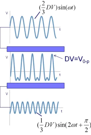
With G3, the standard glass transfer capillary of the source was replaced with a custom flared glass transfer capillary5 to improve ion transmission through the DIMS assembly as compared to the standard capillaries. With G4, a planar flare (Figure 2.2e) was implemented after the electrodes to allow the coupling to a standard transfer capillary while maintaining greater than 80% ion transmission through the assembly in "transparent mode" where both electrodes are held at the same potential. A custom-built power supply6 was used for experiments with G3 DIMS. Ideally, a rectangular waveform should be used for DIMS, alternating between low and high electric fields of opposing polarity. However, because of the power requirements of high voltage, high frequency rectangle waves, most DIMS waveforms are bisinusoidal, approximating a square wave.7 In this design, one sinusoidal voltage at a given frequency and amplitude
is applied to one of the electrodes, and a phase-shifted sinusoidal voltage at twice the frequency and approximately one-half the amplitude is applied to the other electrode, producing an electric field equivalent to the sum of the two individual sinusoidal
waveforms (Figure 2.3). The dispersion voltage (DV) is defined by the maximum voltage (V0-P) of the bisinusoidal waveform.
The dispersion field (ED) is defined as the DV divided by the gap (g) between the DIMS electrodes. The bisinusoidal DIMS
22
waveform was tuned to a frequency of 1.7 MHz with G3 and 2 MHz with G4. For example, with G4 the addition of a sinusoidal wave at 2 MHz and a lower amplitude sinusoidal wave at 4 MHz is used to form the bisinusoidal DIMS waveform at frequency of 2 MHz. A LabVIEW program linked to the instrument control software is used to control the range of compensation voltages or to define a static value. In "scanning mode", the compensation field, EC, is stepped over a range specified in a LabVIEW program. A static voltage can be selected to operate DIMS in "filter mode".
To use ESI with DIMS, a voltage difference of 4.25 kV between the emitter and the DIMS electrodes is applied. The DIMS electrodes are at the same potential as the transfer capillary, to which the ESI voltage is applied without DIMS. With G3, the ESI voltage must be applied to the ESI emitter rather than the DIMS electrodes because the DIMS waveform cannot be superimposed upon a high voltage with G3. A second custom power supply was designed for G4 so that the DIMS waveform can be centered about the ESI voltage and operated with the ESI emitter at ground potential. The same basic design for the application of the bisinusoidal waveform was used, but modifications were made to the power supply as well as the DIMS assembly itself to prevent arcing and to prevent drift in the applied EC.
2.3.2 Trapped Ion Mobility Spectrometry
23 used to focus ions within the analyzer
region. The temperature in the analyzer for all TIMS experiments was 304 K. The fill time for the analyzer is typically a few milliseconds, (10 ms for the experiments in this dissertation) followed by a trapping period to allow ions to separate based on low-field ion mobility, which is proportional to the collision cross-section of ions. Finally, the ions are ramped out of the analyzer section from low to high mobility (large to small cross-sections) by decreasing the voltage difference between the 1st (ramp electrode) and last electrode (exit
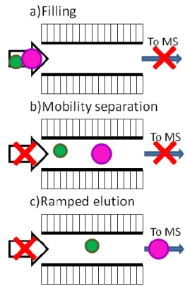
Figure 2.5 Simplified representation of TIMS separations; a) filling, b) ion mobility separation, and c) ramped elution of ions from low to high mobility. Gas flow indicated by arrows.
24
electrode) in the analyzer section. The three steps for the TIMS separation are depicted in Figure 2.5.
With TIMS there is no direct way to determine ion mobility from the TIMS scan so calibrants must be used to determine ion mobility and collision cross-section. Agilent ESI tuning mix (section 2.1.1) was used for the calibrant, for which the ion mobility in nitrogen gas was determined in a drift-tube ion mobility spectrometer (Table 2.3).8 The same tuning mix (m/z 322, 622, 922, 1222, 1522, and 1822) was analyzed with TIMS to create a
calibration plot (Figure 2.6) of K0 versus inverse voltage, where voltage is the voltage difference between the first and last electrodes of the analyzer section. The collision cross-section (CCS) of analyte ions was determined using the calibration plot to convert inverse voltage to K0, followed by the use of Equation 2.1,10,11 where K0 is the reduced ion mobility at standard temperature (T0) and pressure (P0), T is temperature, N0 is the number density at standard temperature and pressure, e is the charge of the ion, µ is reduced mass, kB is Boltzmann's constant, and Ω is the collision cross-section of the ion.
25 2.4 Data analysis
DIMS spectra were constructed by plotting the extracted ion current or total ion current from the Bruker Data Analysis 4.1 software as a function of analysis time. Several time-to-voltage points were recorded during each DIMS scan to be used to convert the time axis of the chromatogram to voltage in Excel.
Each time point in the exported ion current is an average of ten mass spectra, and each time point is equivalent to one CV step, where the step size is specified in the LabVIEW program.
Figure 2.6 Calibration plot used for TIMS experiments correlating reduced ion mobility to inverse voltage.
26
The conversion is applied by using one time-to-voltage point and then the voltage step size is used to determine the voltage at each previous and subsequent time point. The other time-to-voltage points are used to confirm that there is no error in using the step size throughout the time-to-voltage conversion in the DIMS scan. The determined compensation voltage for each time point is then divided by the gap size of the DIMS device to convert to
compensation field for the x-axis of the DIMS spectra. The peak width (w), full-width at half-max (FWHM), and centroid EC for DIMS peaks were determined using the Fit Gaussian function in Origin 6.0. The following three equations are used throughout this dissertation to evaluate DIMS separations: resolving power (RP), resolution (R), and percent ion
transmission (%T):
(Equation 2.2)
(Equation 2.3)
27
2.5 REFERENCES
1. Fmoc solid phase peptide synthesis : a practical approach; Oxford University Press: Oxford; New York, 2000.
2. Louris, J.N.; Cooks, R.G.; Syka, J.E.P.; Kelley, P.E.; Stafford, G.C.; Todd, J.F.J.: Instrumentation, applications, and energy deposition in quadrupole ion-trap mass spectrometry. Anal. Chem., 59, 1677-1685 (1987)
3. Roepstorff, P.; Fohlman, J.: Proposal for a common nomenclature for sequence ions in mass spectra of peptides. Biomedical Mass Spectrometry 11, 601 (1984)
4. Biemann, K.: Contributions of mass spectrometry to peptide and protein structure. Biomedical and Environmental Mass Spectrometry 16, 99-111 (1988)
5. Bushey, J.M.; Kaplan, D.A.; Danell, R.M.; Glish, G.L.: Pulsed Nano-Electrospray Ionization: Characterization of Temporal Response and Implementation with a Flared Inlet Capillary. Instrum. Sci. Technol. 37, 257-273 (2009)
6. Ridgeway, M. E.; Glish, G. L. In preparation
7. Purves, R. W.; Guevremont, R.; Day, S.; Pipich, C. W.; Matyjaszcyk, M. S. Mass spectrometric characterization of a high-field asymmetric waveform ion mobility spectrometer. Rev. Sci. Instrum. 69, 4094-4105 (1998)
8. Hernandez, D.R.; DeBord, J.D.; Ridgeway, M.E.; Kaplan, D.A.; Park, M.A.; Fernandez-Lima, F.: Ion dynamics in a trapped ion mobility spectrometer. Analyst, 139, 1913-1921 (2014)
9. Fernandez-Lima, F.; Kaplan, D.A.; Suetering, J.; Park, M.A.: Gas-phase separation using a trapped ion mobility spectrometer. Int. J. Ion Mobil. Spectrom. 14, 93-98 (2011) 10.McDaniel, E.W.; Mason, E.A.: Mobility and diffusion of ions in gases; John Wiley and
Sons, Inc., New York, NY, 1973, p. 381.
CHAPTER 3: OPTIMIZATION OF DIMS SEPARATIONS 3.1 Evaluation of DIMS separations
In the optimization of any analytical technique, both sensitivity and resolution must be taken into consideration. DIMS separations are often evaluated by calculating the resolving power (RP) of a given peak (Equation 3.1). The RP essentially describes how narrow a given peak is by deteriming the ratio of the peak centroid to the full-width at half-maximum. RP is inherently biased such that if two peaks have the same width, but one has a higher centroid CV than the other, then the peak with the higher centroid will have the higher RP. Resolution (R), which is commonly used for chromatographic separations, provides an evaluation for the separation of two peaks (Equation 3.2). For R, the centroid and width of both peaks are taken into account to determine how well they are separated, where a value of <0.5 indicates that the two peaks overlap significantly and a value of >1.5 indicates that the peaks are baseline resolved.
(Equation 3.1)
(Equation 3.2)
29
the mass spectrometer and converting to a percentage (Equation 3.3). This value is generally calculated for a specific ion, where the extracted ion current for the mass-to-charge of the analyte ion is used for the signal intensity. For %Ttrans, the numerator is the signal obtained for DIMS in transparent mode, where no rf is applied to the electrodes and all ions are allowed to pass through the device without ion mobility separation. For %Tactive, the
numerator is the signal obtained for a given ion at the peak EC for that ion. With both %Ttrans and %Tactive, the denominator is the signal obtained with the device removed from the inlet of the mass spectrometer.
(Equation 3.3)
All of the above values are useful in the evaluation of DIMS separations and can be used in the optimization of various parameters. As discussed previously (1.3.1), DIMS separation power can be affected by the dispersion field,1-3 separation time,4,5 carrier gas temperature and pressure, and carrier gas composition.6-8 The separation time is varied by changing the length of the DIMS electrodes. The carrier gas settings are also examined, where
temperature and percent helium in nitrogen are varied.
3.2 Electrode dimensions
3.2.1 Ion transmission with DIMS transparent
Generation 3 (G3) of the planar DIMS assembly allows for the gap between the electrodes to be easily changed between 0.3, 0.5, and 1.0 mm. Additionally, two different housing sizes, one of which can hold 50 mm long electrodes and the other can hold 25 mm long electrodes, were developed. When the electrodes are lengthened, the ion transit time through the
30
to diffusion is expected. When the gap between the electrodes is increased, the volume within the device is increased, and because the volumetric flow rate of the carrier gas dictates ion transit time, ion losses due to diffusion will increase. Because the DIMS electrodes are coupled to a glass capillary (length=18 cm, i.d.=0.5 mm) that transfers ions from atmospheric pressure to vacuum, a conductance limit of approximately 1.4 L/min dictates the volumetric gas flow rate through the assembly. This gas flow is what carries ions through the assembly, thus determining the ion transit time. Therefore, if the volume between the electrodes is increased, the transit time through the assembly will increase proportionally, allowing for greater ion losses due to diffusion.
Table 3.1 summarizes the %Ttrans determined for the tetrabutyl ammonium ion (m/z 242), angiotensin I3+ (m/z 433), and brain natriuretic peptide (BNP)5+ (m/z 649) for DIMS transparent compared to the assembly removed. A significant difference in ion transmission is observed between the four electrode dimensions used for these experiments. The trends observed are as expected for all ions investigated, where the ion transmission
decreases as the volume between the electrodes is increased. The tetrabutyl ammonium ion has a similar ion transmission between the two gap sizes with the 25 mm long electrodes, with fairly large standard deviations due to the overall low signal observed with the DIMS device attached. The low ion transmission for the tetrabutyl ammonium ion is expected because it is a
31
mass ion compared to the others investigated and will have more diffusion losses as it passes through the DIMS assembly.
3.2.2 Ion transmission with active DIMS: generation 3
The %Ttrans for DIMS transparent is an important piece of information, but it is also critical to evaluate the %Tactive for active DIMS, where the signal for the ion of interest is selected with a given dispersion field (ED) and compensation field (EC), and is then compared to the signal obtained without the DIMS assembly attached. With DIMS active, losses due to diffusion are expected as observed with DIMS transparent because whether DIMS is active or transparent, there is no voltage applied perpendicular to the electrodes, so lateral diffusion remains. In addition to ion losses due to lateral diffusion, ions can collide with the electrodes and be neutralized.
32
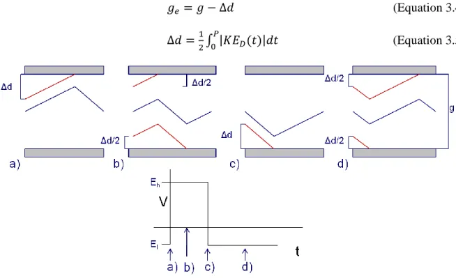
upper electrode a distance of Δd before the waveform returns to El. If an ion enters the gap at a distance of Δd or less from the upper electrode, it will be neutralized on the upper electrode during the first period of the waveform. Ions entering the gap at any other point between the electrodes will be allowed to pass through the DIMS assembly. Thus, the effective analytical gap (ge) can be described by equation 3.4, and Δd is described by equation 3.5, where P is one period of the waveform and K is the ion mobility.1 Ions with a given Kh-Kl can be visualized as an ion beam traversing between the electrodes, with a width equal to ge. The effect of constraining ge is represented in Figure 3.2.
(Equation 3.4)
(Equation 3.5)
With DIMS active, as the physical gap between the electrodes is increased, so too is the effective analytical gap, assuming the dispersion field is constant. Therefore, a greater number of ions can be expected to pass through the assembly with the large gap size than is expected with the smaller gap size. This improvement in ion transmission is in opposition to
33
the expected ion losses due to lateral diffusion, where greater losses are expected for the larger transit time with the larger gap size.
Figure 3.2. A simplified visualization of a constrained effective analytical gap, where (a) is a given separation of ion beams of varying Kh-Kl and (b) is the separation of the same set of ion beams with a constrained effective analytical
gap.
34
enhanced ion transmission of the shorter assembly over the longer assembly (Figure 3.3c-d).
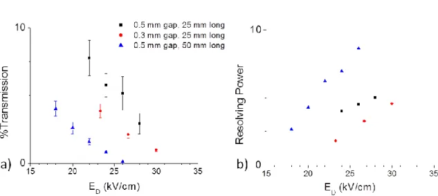
The ion transmission and resolving power for active DIMS was determined using tetrabutylammonium chloride (TBACl) with three of the different electrode sizes (Figure 3.4). The %Tactive for the singly charged tetrabutylammonium ion (m/z 242) with the 0.5 mm gap was greater than that observed with the 0.3 mm gap for the 25 mm long electrodes. The 50 mm long electrodes gave lower %Tactive than the 25 mm long electrodes. As discussed for
35
angiotensin3+, the RP is maximized by using the longer electrodes at each dispersion field, but with a lowered ion transmission.
The effect of changing the gap size between the electrodes was also investigated with brain natriuretic peptide (BNP), a biomarker for congestive heart failure which will be
discussed further in Chapter 5. Utilizing a dispersion field of 30 kV/cm, the separation of the +5 charge state of BNP in a fetal bovine serum (FBS) extract was compared for the 0.3 (Figure 3.5a) and 0.5 mm (Figure 3.5b) gap sizes. The 0.5 mm gap provided a significant improvement in both ion transmission and resolving power over the 0.3 mm gap size, where a RP of 8 and %T of 0.11% was observed with the 0.3 mm gap, but a RP of 24 and a %T of 83% was observed with the 0.5 mm gap. Because the larger gap size has a larger volume between the electrodes, the ions will have an increased transit time through the assembly. An increase in transit time is expected to improve the separation of ions5 and therefore can explain the improvement in resolving power.
36
3.2.3 From generation 3 to generation 4: ion transmission and resolving power
As discussed previously (2.3.1), generation 4 (G4) DIMS has smaller dimensions than G3, being 10 mm long, 4 mm wide, with a gap of 0.3 mm between the electrodes. Additionally, G4 is coupled to a transfer capillary with an i.d. of 0.6 mm, making the conductance limit 2.9 L/min, as compared to the conductance limit of 1.4 L/min for the capillary used with G3; the increased conductance limit corresponds to an increase in the gas flow between the
electrodes. Due to the smaller dimensions and increased volumetric flow rate of the carrier gas, it is expected that the shorter ion transit time will cause a significant improvement in ion transmission when switching from generation 3 to generation 4. This shorter transit time is also expected to be detrimental to the observed resolving power for a given separation. BNP was used to compare the performance of G3 to G4 (Table 3.2).
Comparing G3 to G4, the primary difference is the electrode dimensions. The RP with G4 is lower than with G3 when compared at the same dispersion field because G4 is
Figure 3.5. Separation of 200 nM BNP5+ in FBS extract with 25 mm long electrodes a) 0.3 mm gap and b) 0.5
37
shorter than G3, causing a decrease in the ion residence time. At the same dispersion field, greater than 100% ion transmission is observed with G4, whereas less than 1% is observed with G3. It should be noted that an ion transmission greater than 100% can be observed because an ion trap was used for these experiments. When background ions are filtered out by DIMS, the finite charge capacity of the ion trap is maximized with respect to the analyte ion, allowing a %Tactive of greater than 100% to be observed (1.3.1). Because the %Tactive was significantly increased, a higher dispersion field was able to be used, while still maintaining nearly 50% ion transmission. Thus, an increase in RP from 8.03 to 21.8 was observed for BNP when analyzed with generation 4.
3.3 Carrier gas parameters 3.3.1 Carrier gas temperature
As described previously (2.3.1), the housing of the DIMS assembly reroutes the desolvation gas already implemented in the source region of the mass spectrometer. This gas serves both as a desolvation gas for ESI as well as being the carrier gas through the DIMS assembly. The temperature (T) was varied from ambient to 106ºC with the protonated peptides YGGFL (m/z 556), AAAAA (m/z 374), and QQQQ (m/z 531). An increase in temperature is expected to increase diffusion (equation 3.6),9 but also decrease low-field ion mobility (equation 3.7).9
Electrode dimensions (mm) ED (kV/cm) %Tactive* at peak EC RP
0.3 x 6 x 25 (G3) 33.3 0.11 8.03
0.3 x 4 x 10 (G4) 33.3 139.0 5.99
50.0 48.8 21.8
38
With DIMS active, an increase in lateral diffusion is expected to decrease the ion
transmission, and a decrease in ion mobility is expected to increase the ion transmission due to an increased ge.
Equation 3.6
Equation 3.7
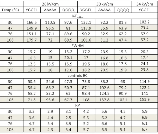
In addition to investigating the ion transmission as a function of the carrier gas temperature, resolving power is an important parameter to consider. For each dispersion field, %Tactive, FWHM, peak EC, and RP were determined for protonated YGGFL (m/z 556), AAAAA (m/z 374), and QQQQ (m/z 531) (Table 3.3). For each dispersion field used, the RP increased with increasing carrier gas temperature. An increase in desolvation gas
temperature is expected to cause more complete desolvation of the ions formed by ESI. Bare, desolvated ions are expected to undergo more elastic, hard-sphere collisions with the carrier gas than solvated ions. The hard-sphere scattering model for ion-drift gas interactions predicts a decrease in ion mobility with increasing electric fields (KH < KL). 6 Peptide and protein ions exhibit a decrease in ion mobility with increasing electric fields in a nitrogen carrier gas, which in our assembly corresponds to a positive EC value that increases with increasing dispersion fields.
DIMS is open to the atmosphere and therefore a change in temperature causes a change in the number density (N) of the buffer/carrier gas, where T and N are inversely proportional. Ion mobility is proportional to E/N,9 increasing temperature is observed to have a similar effect on DIMS separations as increasing the dispersion field. Both
39
positive) EC to be selected using DIMS. Therefore, an increase in RP is expected with increasing temperatures which was observed for protonated YGGFL, AAAAA, and QQQQ.
3.3.2 Desolvation gas flow rate
With the DIMS design used for these experiments, the desolvation gas flow can be varied to manipulate the temperature of the carrier gas between the electrodes of the DIMS assembly. With a desolvation gas temperature setting of 300 ºC, the temperature of the electrodes is 53ºC at a flow rate of 2.5 L/min, 84ºC at 5 L/min, and 111ºC at 7.5 L/min. With an increase in the temperature, the gas number density in the analytical gap decreases because the
Table 3.3. %Tactive, FWHM, centroid EC, and RP for protonated YGGFL (m/z 556), AAAAA (m/z 374), and
40
pressure is constant. Thus, E/N increases with increasing carrier gas temperature causing a shift in the observed EC of a given ion. The default desolvation gas flow rate is 5 L/min and was used for all experiments when not specified. Using a mixture of YLFTLEPQT and LLSLLLLMPV, which are isobaric peptides with a nominal molar mass of 1111 Da, the resolution between the two peaks was determined at various desolvation gas flow rates, using 100% nitrogen and a fixed ED of 72 kV/cm (Figure 3.6). These data confirm that for these isobaric peptides, the resolution increases from 0 to 1.26 as the desolvation gas flow rate increases from 2.5 to 7.5 L/min at a constant ED. As with the increased electric fields, increasing the temperature within the gap causes a decrease in ion transmission through the DIMS assembly.
Figure 3.6 DIMS scans obtained as desolvation gas flow rate is varied at a fixed ED of 72 kV/cm (a) 2.5 L/min, (b) 4
L/min, (c) 5 L/min, (d) 6 L/min, and (e) 7.5 L/min. Resolution was calculated at each flow rate.
300 400 500
0.0 1.0x10⁵ 1.5x10⁵ 2.0x10⁵ 3.0x10⁵ 3.0x10⁵ (e) (d) (c) (b) (a) E
C (V/cm)