4898.pdf

(1)

Systematic approaches to integrate inconsistent, noisy

high-throughput data to bolster subtle relationships

obscured by standard analyses

Jennifer M. Staab

A dissertation submitted to the faculty of the University of North Carolina at Chapel Hill in partial fulfillment of the requirements for the degree of Doctor of Philosophy in the Depart-ment of Computer Science.

Chapel Hill 2012

Approved by:

Shawn M. Gomez

Wei Wang

Jan F. Prins

Leonard McMillan

(2)

c

(3)

Abstract

JENNIFER M. STAAB: Systematic approaches to integrate inconsistent, noisy high-throughput data to bolster subtle relationships obscured by standard analyses.

(Under the direction of Shawn M. Gomez.)

The increasing availability and decreasing cost of high throughput technologies coupled with the

availability of computational tools form a basis for a shift to a more integrated approach to analyzing

biological processes. In particular, classical statistical analysis techniques are designed to analyze data

characterized by a single data source and are distinguished by a much higher ratio of subjects to the

number of observations. In contrast, bioinformatics and systems biology applications often involve

large data sets characterized by an abundance of observations spawned from a relatively small sample

of subjects. The complexity of these systems coupled with the need to integrate inconsistent (noisy)

data require appropriate methodologies that address these issues.

Standard analyses can proficiently identify associations within consistent data, but these approaches

are not robust at identifying relationships across data sources and/or where nontrivial amounts of

in-consistency (noise) are present. Such data requires approaches that account for this increasing

incon-sistency within the data. One technique of accounting for such inconincon-sistency is to limit analyses to

subsets of data where the desired associations are the most prominent. Challenges for this particular

approach involve the determination of subsets of interest while simultaneously establishing a metric

with which to judge statistical importance.

My initial work using this approach involved providing a methodology to represent Nuclear

Mag-netic Resonance (NMR) Spectra as hundreds of aligned peaks as opposed to thousands of unaligned

points, which allows for more sophisticated means of analysis. My later work explores the

develop-ment of data mining methodologies for identifying associations that exist within subsets of

inconsis-tent, noisy data while addressing how to sensibly target subsets of interest while establishing a metric

of association that provides statistical significance. Two approaches were developed, the first of which

established a p-value associated metric, while the latter allowed for multiple arbitrary metrics of

inter-est to be used to identify statistically significant patterns. This work helps to inter-establish methodologies

(4)

Acknowledgments

My gratitude goes out to my advisor Dr. Shawn Gomez for his guidance and support throughout

the course of my dissertation research. I am also grateful to Dr. Thomas O’Connell for his invaluable

guidance and collaboration within the field of metabolomics and with PCANS. I am thankful to the

rest of my committee, Dr. Wei Wang, Dr. Jan Prins and Dr. Leonard McMillan, for the feedback and

advice they provided regarding my research and defense.

I am grateful to my longtime friend, officemate, and colleague, Kwangbom Choi, whose counsel

and camaraderie throughout our graduate careers has proved to be an invaluable resource. I am thankful

to the members of the Gomez Lab, Matt Berginski, Alicia Midland, Janet Doolittle and Ke Xu, whom

have provided valuable friendship, feedback, and support throughout our shared lab experience. I am

also thankful to my fellow bioinformatics and computational biology colleagues past and present whom

have provided support and encouragement during my graduate career.

I am most grateful to my family and friends whose encouragement and support over my long

grad-uate career have made this achievement possible. My parents for their unwavering and unconditional

support, despite not fully understanding what I was working on and why it was important to me. My

sister whom has always been there at the ready with advice, encouragement, and veterinary assistance

at all hours of the day. My brother and nephews whom have provided the much needed

extracurricu-lar breaks to view hockey games. I am thankful to Scott and the Reidsville cycling crew whom have

provided endless hours of extracurricular distraction via cycling and encouragement of my academic

pursuits. I would also like to thank my longtime friends, Marisa, Jiten, and Trang, although not directly

associated to academia they have provided much needed encouragement and support over the years.

And a special thanks to Jim, for the much needed late night laughs, friendship, encouragement, and

(5)

List of Tables

3.1 Quantification of EPA’s ToxCast and ToxRefDB data . . . 53

4.1 Closed & Approximate Itemsets by Seed Node . . . 90

4.2 Chemicals Common to Significant Sets associated with

Rat Skeletal Development and Liver Lesions . . . 94

4.3 Chemicals Common to Significant Sets associated with

Rat and Mouse Liver Lesions . . . 100

4.4 15 Top Scoring Biclusters found with BicBin Algorithm . . . 102

4.5 Comparison of Closed/Approximate Itemset Mining to

BicBin Biclustering for All & Approximate Subsets . . . 103

4.6 Timing of Closed Frequent Itemset Mining using

Differ-ent Support Thresholds on ToxCast Data . . . 107

5.1 Statistics on Significant Rules given FDR Adjustment atα0.05 . . . 132

5.2 Rule and Timing Statistics Bootstrap Samples for Rules

(10)

List of Figures

2.1 Overview of the PCANS Alignment Process . . . 16

2.2 Final Consensus Profile Formation . . . 20

2.3 Accuracy of alignment as a function of scoring weights assigned to peak attributes . . . 21

2.4 Accuracy of Alignment with Simulated Peak Profiles . . . 31

2.5 Standard deviations corresponding to the alignment accuracies shown in Figure 2.4 . . . 32

2.6 A Sample Region of Simulated Peak Profiles Before and After Alignment . . 34

2.7 PCA Analysis of Simulated Peak Profiles . . . 36

2.8 Loadings Plots of Simulated Peak Profiles . . . 37

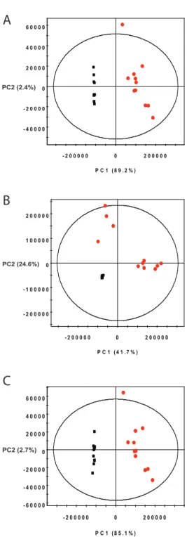
2.9 PCA Analysis of Mouse Urine Spectra . . . 40

2.10 Loadings Plots of Mouse Urine Peak Profiles . . . 41

2.11 OPLS Analysis of Mouse Urine Spectra . . . 43

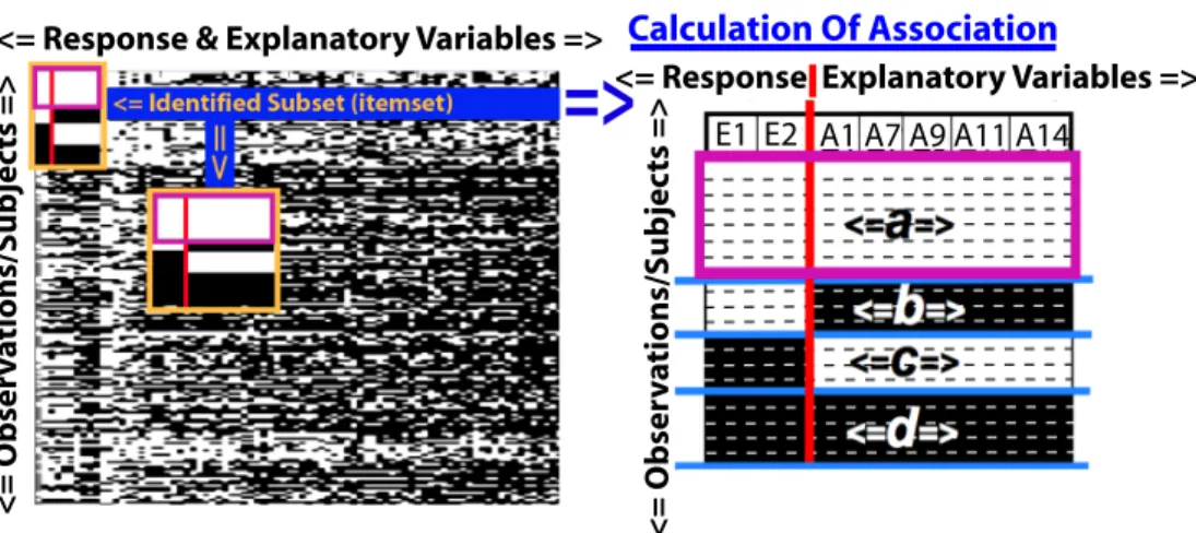
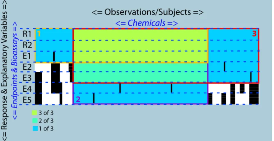
3.1 Subset Combinations Depiction . . . 64

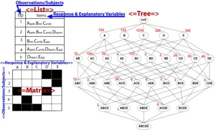
4.1 Subsetting Binary Data with Frequent Itemset Mining . . . 68

4.2 Itemset Mining Definitions . . . 69

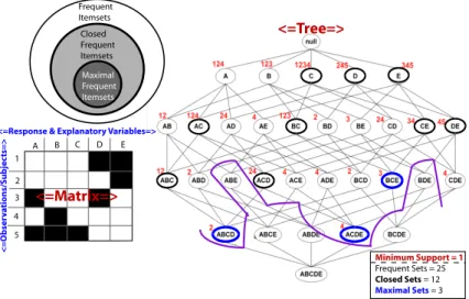
4.3 Efficiencies of Closed Frequent Itemset Mining . . . 72

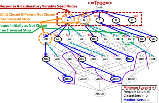
4.4 Closed Frequent Itemset Mining to Identify Subsets within Binary Data . . . 76

4.5 Overlapping Closed Itemsets . . . 77

4.6 Mining for Approximate Frequent Itemsets . . . 81

4.7 Statistic of Association . . . 85

(11)

4.9 Rat Skeletal Development and Liver Lesions Tree . . . 91

4.10 Rat Skeletal Development and Liver Lesions Heat Map All Chemicals . . . . 93

4.11 Rat Skeletal Development and Liver Lesions Heat Map Select Chemicals . . . 95

4.12 Rat and Mouse Liver Lesions Heat Map All Chemicals . . . 98

4.13 Rat and Mouse Liver Lesions Heat Map Select Chemicals . . . 99

4.14 Comparison of Closed/Approximate Itemset Mining to BicBin Biclustering for All Subsets Classified by Num-ber of Endpoints . . . 104

4.15 Timing Plotted for Closed Itemset Creation . . . 106

5.1 Issue with using statistics based upon p-value . . . 110

5.2 Association for Multiple Data Sources . . . 111

5.3 Creation of Rules (Subsets) from Transaction Set (Dataset) and Calculation of the Metric for each Rule . . . 114

5.4 Bootstrap Sample Creation using Original Transaction Set (Dataset) and Summarization to findε(δ)Threshold . . . 115

5.5 ToxCast Closed Itemsets that create Simulated Data . . . 119

5.6 Significance Thresholds based upon FDR and Bonferroni Correction on the Simulated Dataset . . . 120

5.7 Verification of Bootstrap Method . . . 122

5.8 Verification of the Rescaling Metrics . . . 127

5.9 Bootstrap Results using Scaled Consistency and Scaled Composite Metrics on the Simulated Dataset . . . 129

5.10 Threshold Problem with ToxCast Data . . . 131

5.11 Rules Reduction Solution to Threshold Problem . . . 133

5.12 Lower Comparison Threshold Solution to Threshold Problem . . . 135

5.13 Bootstrap Results fromScaledConsistency Metric using ToxCast Data . . . . 137

(12)

Chapter 1 Introduction

1.1 Motivation and Goals

The increasing availability and decreasing cost of high-throughput (HT) technologies coupled

with the availability of computational tools and data form a basis for a shift to a more

in-tegrated approach in analyzing biological processes. Classical statistical analysis techniques

were designed to analyze data characterized by a single data source distinguished by a much

higher ratio of subjects in comparison to the number of observations arising from each subject.

In contrast, bioinformatics and systems biology often involve high-throughput data

character-ized by an abundance of observations spawned from a relatively small sample of subjects.

Additionally, the complexity of these systems under analysis coupled with the need to in-tegrate inconsistent (noisy) data often violates many of the assumptions of classical analytic

techniques. My primary focus has been based upon the identification of relationships amongst

noisy, inconsistent data within the context of providing a more integrated approach to

analyz-ing biological processes. The approaches I developed identify subsets of data that maintain

robust analytic relationships obscured by the standard methodologies.

My initial work was within the field of metabolomics and focused on providing a

(13)

integration of metabolomic data and aid their incorporation into larger integrative analysis

frameworks. Specifically, the transformation of the spectrum representation from points to peaks which reduces the inconsistency within a spectrum by focusing directly on the

compo-nent of analysis. The algorithm reduces each spectrum from thousands of points to hundreds

of consistent peaks for final analysis. Moreover, the automated alignment of the NMR spectra

served as a means of further noise reduction, increasing the likelihood that the peaks within

each spectrum would be fruitful with regards to the final result. The noise reduction provided

by this transformation and alignment process greatly simplified data complexity and enabled

further application of other means of statistical analysis of NMR spectra.

From this, my focus shifted to developing data mining methods to identify relationships that exist within subsets of inconsistent, imperfect data. My research deliberately focused

upon data where traditional means of analysis proved to be futile, to identify association

between response and explanatory variables as data sources are integrated over a common

set of subjects. Specifically, the toxicological associations between animal study endpoints

(response variables) and high-throughput/high-content bioassays (explanatory variables) as

perturbed by the same potentially toxic chemicals (subjects). The methods I employed use

pattern identification approaches to identify subsets of potentially toxic chemicals that per-turbed sets of animal endpoints and bioassays in a consistent manner. These methods have

been enhanced to allow for the incorporation of user-defined amounts of fuzziness into the

re-sults and to enable the identification of statistically significant rere-sults based upon user defined

metrics (no p-value required). Furthermore, the methods can be employed upon larger, more

dense datasets through targeted analysis and can be used in the integration of three or more

(14)

1.2 Brief Overview of Existing Methods

1.2.1 NMR Spectra Noise Reduction Methods

As discussed in detail in Chapter 2 within the field of metabolomics, the standard way to

reduce the noise in spectra prior to analysis is through binning, a procedure that involves

di-viding the spectra into small windows and taking the area under the curve for each window as the final intensity (Gartland et al., 1991; Anthony et al., 1994). Ideally, these windows will

be large enough to encompass peak drift and to reduce the number of points that represent a

spectrum, but not so large as to include many peaks in a single bin. The latter consequence is

unavoidable in crowded spectra and thus there is the potential for significant loss of

informa-tion when binning, for example by including peaks belonging to multiple compounds within a

single bin. Alternatives to binning typically involve some form of peak alignment procedure.

Several algorithms have also been recently developed to align peaks in sets of NMR spectra Wu et al. (2006); Kim et al. (2006); Torgrip et al. (2003); Veselkov et al. (2009); Savorani

et al. (2010).

Current advanced NMR alignment methods such as fuzzy warping (Wu et al., 2006),

Bayesian alignment (Kim et al., 2006), Recursive Segment-Wise Peak Alignment (Veselkov

et al., 2009), peak alignment by FFT (Wong et al., 2005; Savorani et al., 2010) and peak

align-ment using reduced set mapping without recursive target update (Torgrip et al., 2003), are

based on the use of a template spectrum to help align a set of spectra. Choosing a template typically involves either selecting a single sample spectrum that appears most like the others

as determined by some measure of similarity, creating an ”average” spectrum, or by choosing

a reference spectrum not contained within the sample. All remaining sample spectra are then

aligned to this selected template using some form of pairwise alignment algorithm. A

signif-icant problem with the template approach is that there can be a great amount of variability

between any two spectra. Part of this difference arises due to the previously described

(15)

groups within the data; for instance, inter-group variation between control and treated groups,

subpopulation differences within these groups, etc. There may often be a priori knowledge of general subgroups, but one of the goals of metabolomics is to discover new subgroups

such as different types of responders in drug or toxicity studies; by definition, templates for

such groups are not known beforehand. Thus in such cases, the use of a template can

signif-icantly complicate downstream analyses. Further discussion of existing methodologies and

comparison of these methodologies to our own can be found in Chapter 2.

1.2.2 Identifying Association in Inconsistent, Noisy Data

Clustering is a fundamental method of unsupervised learning that partitions data in a way as to

highlight meaningful relationships by exploring how data groups based upon similarity. Given a two-dimension data matrix, 2-D hierarchical clustering can be used to consider both columns

and rows of the data when looking for meaningful relationships within the data. 2-D

hierar-chical clustering is not ideal in inconsistent, noisy data because the methodology considers the

entire record (all the data in a given row and for a given column) when partitioning the data

into meaningful groups. Similarly to 2-D hierarchical clustering, biclustering is able

concur-rently partition data by both rows and columns. Unlike 2-D hierarchical clustering,

bicluster-ing is able to consider submatrices, or subsets of the data; thus, usbicluster-ing biclusterbicluster-ing is a better method than hierarchical clustering to identify meaningful relationships within inconsistent

data. Computationally, biclustering works best on sparse data matrices or when heuristics are

used to limit the exhaustive enumeration of all possible submatrices. This is because

biclus-tering solutions employ algorithms with computational complexity of NP-complete, meaning

they have no known polynomial time algorithms and in the worst case their runtimes are

ex-ponential. van Uitert et al. (2008) demonstrate the use of biclustering on high-throughput data

when they employ their method of biclustering on sparse binary genomic data to identify in-teracting transcription factors. Another example is DiMaggio et al. (2010) use of biclustering

(16)

between sets of explanatory variables and a response variables. Methods of biclustering most

directly compare to our methodology because they focus upon analysis of subsets of the data. Other methods of determining association across multiple datasets with inconsistent data

typically involve a bayesian framework. Specifically, these methods tend to weight the data

based on its usefulness in the underlying mathematical model of association as was

demon-strated by Webb-Robertson et al. (2009) using metabolomic data. The primary motivation of

the study by DiMaggio et al. (2010) was to identify relationships between explanatory and

response variables that could be used in prediction; whereas, the motivation of the

Webb-Robertson et al. (2009) methodology was to identify relationships that provided the most

sig-nificant differences between classes based upon integrated metabolomic data. Zhang et al. has developed data mining methods to identify significant relationships that existed between sets

of explanatory and response variables for categorical data (Zhang et al., 2010b,a). Similarly,

van Uitert et al. (2008) developed a method that was used to determine an association between

two sets of genomic data to identify clusters with novel associations between the datasets.

Al-though not focused on the relationship between explanatory and response variables, Reif et al.

(2010) developed a measure that integrates multiple sources of toxicological data together

to prioritize toxicological risk. Unlike DiMaggio et al., the methodology of Zhang et al. is able to integrate together the search for relationships with significance testing of discovered

relationships. DiMaggio and Webb-Robertson both use methods that are more suited for

in-tegrating data from multiple data sources where a high degree of inconsistency (noise) exists

between the data sources. Additionally DiMaggio, Webb-Robertson, and Reif’s

methodolo-gies are more suitable for handling numeric data as compared to the methods that Zhang et

al. employ which involve pairwise association between categorical data. The methodology of

van Uitert et al. addresses some degree of inconsistency within the data, but unlike the other methods, its primary goal is the discovery of novel associations identified through integration

with little regard for finding all associations or assigning statistical significance to the results.

(17)

indicate the importance of its results. However, their methodology does provide a ranking of

toxicological risk based upon multiple data sources. As discussed above there are multiple methods of integrating inconsistent data, but the biclustering methodology (like van Uitert

et al. (2008)) is most similar to our methods because they both focus upon analysis of subsets

of data to deal with inconsistency.

1.3 Approach and Innovations

1.3.1 Methods to Enhance NMR Spectra Analysis

Our novel approach for the alignment of NMR spectra is based on the creation of a

consen-sus spectrum alignment through integration of pairwise spectrum comparisons (referred to as

PCANS hereafter - Progressive Consensus Alignment of Nmr Spectra). To our knowledge,

this is the first such consensus approach applied to the alignment of NMR spectra and the only approach that transforms spectra from points to peaks prior to alignment as opposed to

using the entire spectrum. This approach has several advantages that include the ability to

align spectra with significant amounts of noise in chemical shift position, peak height and

peak width. By using peaks as the basis for alignment we maintain the maximally informative

set of information existing within a set of spectra. As a result, the existence of subgroups

within a set of spectra can be identified since group-specific peaks are maintained in the final

alignment.

We characterize the performance of this approach by aligning simulated NMR spectra

which have been provided with user-defined amounts of chemical shift variation as well as

inter-group differences as would be observed in control-treatment applications. Moreover,

we demonstrate how our method provides better performance than either a template-based

alignment or binning. Finally, we further evaluate this approach in the alignment of real

mouse urine spectra and demonstrate its ability to improve downstream statistical analyses

(18)

1.3.2 Methods to Enhance Association Identification

The data mining methods implemented focus on data where traditional methods of

predic-tive modeling failed to identify useful relationships because they considered the entire data record. In contrast our approach, similar to biclustering, identifies relationships amongst

sub-sets of the data. Our methods differ from the biclustering and prediction scheme of DiMaggio

et al. (2010) by allowing one to incorporate group identification and association in a more

streamlined framework. Moreover, our methods exhaustively explore the inclusion of

mul-tiple response variables with regards to association with the explanatory variables, while the

work of DiMaggio et al. considers each response variable separately. Our methods more

fully explore all possible enumerations of the subsets of data that specifically support the desired association; in our case the association between response and explanatory variables.

Our methods are more similar to those employed by Zhang et al. (2010b,a) with regards to

incorporating association finding and significance into a streamlined framework. However,

unlike Zhang, our methods focus on subsets of the data (Zhang et al., 2010b,a). While our

algorithms are similar to the methodology of van Uitert et al. (2008) as in they are applied to

sparse inconsistent binary data; they differ from this work in that they provide a measure of

statistical significance for the results. Additionally they provide the full complement of results

for a given threshold, and can be modified to integrate more than a pair of datasets. Our meth-ods differ from all three (Zhang, DiMaggio, Webb-Robertson) by allowing one to incorporate

fuzziness (allowable zeros) given specific restrictions (described later). Finally, our algorithm

is able to be applied to the mining of larger datasets by constraining the search space through

requiring a minimum number of pre-specified features in the output through the use of seed

nodes.

1.3.3 Thesis

Classical statistical analyses are not robust in identifying relationships within data in the

(19)

consistency, I develop methods that show improved identification of relationships as evidenced

by the relevance of the generated results.

The methods I develop focus on two areas of research, NMR spectra analysis and data

mining for association within inconsistent data. The contributions to improving NMR spectral

analysis are discussed first. The data mining for association follows because these methods

can be directly applied to NMR spectral analysis to improve the relevance of the results.

1.3.4 Contributions to Enhance NMR Spectra Analysis

To address these problems of inconsistency between NMR spectra when performing

metab-olomic type analysis, our methods transform and align the peaks of each spectrum. This

reduces the analysis to a small subset of well-aligned aligned peaks as opposed to attempting to quantify and analyze all the unaligned points of each spectrum. Treating each spectrum as

hundreds of aligned peaks as opposed to thousands of unaligned points enhances the analysis

we can perform and enables us to use more sophisticated means of analysis as is discussed in

detail in Chapter 2.

Innovations made with regards to NMR spectra analysis are the following:

• Spectra are transformed (subset) to a collection of peaks with properties of location,

height and width instead of a collection of points

– Reduces spectrum to relevant information

– Reduces complexity of alignment and analysis

– Reduction allows for more sophisticated analysis

• Alignment algorithm that employs consensus as opposed to template alignment

– Improves quality of alignment by preventing misalignment of peaks not found

within the template

(20)

– Removes need to identify all peaks within sample spectra for template formation

– Same amount of computation as template alignment when coupled with pairwise

alignment schemes

1.3.5 Contributions to Enhance Association Identification

With the integration of datasets over a common set of observations, inconsistencies are

ad-dressed by identifying subsets of data that most strongly support the desired association

be-tween the datasets. For this problem in particular, the methods developed focus on

deficien-cies in current methodologies by identifying consistent relationships within noisy data. Once

these subsets are identified, the methodology establishes a statistical framework under which

the significance of the subsets can be ranked and their strength of association can be deter-mined. This approach of exploring relationships within subsets of the data is meant to be

used when traditional means of analysis fail to produce adequate results due to inconsistency

within the data. Furthermore, this methodology is meant to be used as an exploratory tool to

find underlying relationships that were obscured with traditional means of analysis.

Innovations made with regards to the discovery and prioritization of subsets:

• Determination of Subsets with Closed/Approximate Itemset Mining

– Means to target analysis on certain relationships with use ofseed nodes

∗ Full enumeration of desired relationships based upon frequency criterion

∗ Exploration of larger, more dense data through targeted analysis

∗ Ability to focus analysis on multivariate associations (2+ response variables)

– Incorporation of Fuzziness into subsets

∗ For larger, more dense datasets

∗ Use of statistic to provide relevance of results

(21)

– Strength of association and statistical relevance

∗ Phi Coefficient used to rank and provide statistical relevance for closed /

ap-proximate itemsets applied to identify association between explanatory and

response variables

∗ Established techniques to enable use of bootstrap methodology on larger

data-sets with higher support thresholds to facilitate use of anymetric to quantify

association

– Integration of 3+ Datasets with bootstrap methodology’s use of multiple metrics

1.4 Dissertation Outline

In chapter 2, I describe my initial work on PCANS in the field of metabolomics in detail. Beginning with background and motivation, describing the methodology, results on simulated

and real data, our conclusions and future directions. Chapters 3 through 5 focus on my work

developing data mining techniques to mine for association with inconsistent, noisy datasets.

Chapter 3 describes in detail the background and related work. Chapter 4 describes using

closed/approximate itemset mining in conjunction with the phi coefficient to discover

signifi-cant subsets within data. Chapter 5 describes in detail mining for association with a bootstrap

(22)

Chapter 2 Enhancing Metabolomic Analysis with PCANS

2.1 Background

Continuing technological advances are providing rich data sets quantifying an increasingly

broad range of biological processes. Obvious examples include the use of microarrays for the

quantification of mRNA levels and mass spectroscopy for the identification of protein states

and their interactions. Coinciding with these technological developments are computational

approaches for the extraction, organization and analysis of these data. The application of

improved experimental methods in combination with tailored computational approaches is

providing a major driving force in the development of a more global, systems perspective of

biological function and disease.

Metabolomics, also referred to as metabonomics, similarly provides a comprehensive

pic-ture of biological function by focusing on quantitative measurement of metabolites in

biolog-ical fluids, cells or tissues (Nicholson et al., 1999; Robertson, 2005). The two major

analyti-cal platforms used in metabolomics are nuclear magnetic resonance (NMR) spectroscopy and

mass spectrometry (MS), the latter typically being preceded by either liquid or gas

chromatog-raphy (LC/MS and GC/MS respectively). The ultimate goal of these methods is to extract

(23)

result-ing data is analyzed usresult-ing multivariate methods such as principal components analysis (PCA).

Such analyses typically require significant preprocessing of the data. In particular, it is im-perative that signals for a given compound appear at the same location in all spectra. Signal

locations can vary significantly, however, as in the case of LC/MS where small deviations in

the chromatographic retention time can arise from variation in instrumental parameters such

as flow rate, gradient slope and temperature. In NMR spectra, the peak location can vary

due to differences in pH, ion content and the concentration of metabolites. For both of these

methods, this variability has to be overcome in order to provide a consistent set of spectra for

analysis.

The most common method of addressing variability across spectra is through binning, a procedure that involves dividing the spectra into small windows and taking the area under

the curve for each window as the final intensity (Gartland et al., 1991; Anthony et al., 1994).

Ideally, these windows will be large enough to encompass the peak drift, but not so large as to

include many peaks in a single bin. The latter consequence is unavoidable in crowded spectra

and thus there is the potential for significant loss of information when binning, for example by

including peaks belonging to multiple compounds within a single bin. Alternatives to binning

typically involve some form of peak alignment procedure. For LC/MS methods, a number of algorithms have been developed to align similar peaks across a set of chromatograms (e.g.

(Wong et al., 2005) and recently reviewed in (America and Cordewener, 2008)). Similarly,

several algorithms have also been recently developed to align peaks in sets of NMR spectra

(Wu et al., 2006; Kim et al., 2006; Torgrip et al., 2003; Veselkov et al., 2009; Savorani et al.,

2010). In this paper we describe a novel peak alignment method for NMR that is specifically

tailored to the demands of large and disparate metabolomics datasets.

Current advanced NMR alignment methods such as fuzzy warping (Wu et al., 2006), Bayesian alignment (Kim et al., 2006), Recursive Segment-Wise Peak Alignment (Veselkov

et al., 2009), peak alignment by FFT (Wong et al., 2005; Savorani et al., 2010) and peak

(24)

based on the use of a template spectrum to help align a set of spectra. Choosing a template

typically involves either selecting a single sample spectrum that appears most like the others as determined by some measure of similarity, creating an “average” spectrum, or by choosing

a reference spectrum not contained within the sample. All remaining sample spectra are then

aligned to this selected template using some form of pairwise alignment algorithm. A

signif-icant problem with the template approach is that there can be a great amount of variability

between any two spectra. Part of this difference arises due to the previously described

chem-ical shift variation. In addition, significant differences arise due to the existence of disparate

groups within the data; for instance, inter-group variation between control and treated groups,

subpopulation differences within these groups, etc. There may often be a priori knowledge of general subgroups, but one of the goals of metabolomics is to discover new subgroups such

as different types of responders in drug or toxicity studies; by definition, templates for such

groups are not known beforehand. Thus in such cases, the use of a template can significantly

complicate downstream analyses.

Here we describe a novel approach for the alignment of NMR spectra that is based on the

creation of a consensus spectrum alignment through integration of pairwise spectrum

compar-isons and referred to as PCANS hereafter (Progressive Consensus Alignment of Nmr Spectra). To our knowledge, this is the first such consensus approach applied to the alignment of NMR

spectra. This approach has several advantages that include the ability to align spectra with

significant amounts of noise in chemical shift position, peak height and peak width. By using

peaks as the basis for alignment we maintain the maximally informative set of information

existing within a set of spectra. As a result, the existence of subgroups within a set of spectra

can be identified since group-specific peaks are maintained in the final alignment.

We characterize the performance of this approach by aligning simulated NMR spectra which have been provided with user-defined amounts of chemical shift variation as well as

inter-group differences as would be observed in control-treatment applications. Moreover,

(25)

alignment or binning. Finally, we further evaluate this approach in the alignment of real

mouse urine spectra and demonstrate its ability to improve downstream statistical analyses such as PCA and OPLS models commonly used in metabolomics analyses.

2.2 Methodology

2.2.1 Experimental NMR data collection and processing

Complete details on the urine collection and sample preparation are given in (Bradford et al.,

2008). Briefly, the samples consisted of 540µl of urine plus 60µl of a D2O solution containing

5mM trimethylsilylpropionate-d4 (TSP) as a concentration and chemical shift reference. The

solutions were transferred to 5 mm NMR tubes and NMR spectra were acquired on a Varian

Inova 400 MHz spectrometer using a 5 mm pulsed field gradient, inverse detection probe

(Varian, Inc., Palo Alto, CA). The spectra were acquired with 1024 transients and a sweep width of 4650Hz digitized with 16384 points. The pulse sequence included a 4 second solvent

presaturation period and a 2.6 second acquisition time. A 45 degree excitation pulse was used

to provide quantitative results.

The data were processed using ACD software version 9 (Advanced Chemistry

Develop-ment, Toronto, Canada). A 0.1Hz exponential line broadening was applied to the data. The

spectra were phased and baseline corrected using a 6th order polynomial fitting algorithm

implemented in the software. The spectra were normalized to the integral for the TSP peak. The digitized spectra were exported as text files for subsequent peak picking prior to

align-ment with the PCANS method. Spectral binning was carried out by dividing the spectrum

into uniform 0.04 ppm bin windows and taking the integral value as the sum of the intensities

of all peaks in that bin. The regions from 0.5 to 4.7 ppm and 4.9 to 9.5 were included in the

integration. The regions below 0.5 and above 9.5 contained only noise and the region from

(26)

2.2.2 Multivariate statistical analysis

The statistical analyses were performed using SimcaP+ version 11.5 (Umetrics, Umea,

Swe-den). Pareto scaling was applied to both the peak picked and binned NMR data prior to prin-cipal component analysis (PCA) and orthogonal projection to latent structures discriminant

analysis (OPLS-DA) (Wiklund et al., 2008; Cloarec et al., 2005).

2.2.3 Peak picking

The simulated spectra were based upon peaks manually chosen from an actual urine spectrum.

Peaks were chosen such that they contained a range of features typically found within normal

spectra including tall and small peaks, clusters of many closely spaced peaks, doublets, etc.

These peaks and their associated chemical shift position, height and width were then used

as the basic material from which simulated spectra (peak profiles) were generated. Thus,

the peaks used for simulation are a representative subset of the original spectrum and the

simulation program uses sets of these along with defined amounts and types of variation to

generate the simulated profiles. For simulated spectra, the steps responsible for peak detection and peak attribute assignment are skipped since the simulated spectra are already defined with

a set of peaks with associated attributes.

For real NMR spectra, the peak detection algorithm uses the derivative of the spectrum to

detect and define potential peaks. Potential peaks must have a zero first derivative, a negative

second derivative and be composed of at least 8 points, where points here refer to data values

from the digitized raw spectra. In addition, we use the number of points that define a peak as

well as peak height relative to neighbors to determine ‘real’ peaks from noise peaks within a given spectrum. Specifically, for each potential peak, we look in a region centered around this

point (151 points in this work) and call this a ‘true’ peak if it exceeds a user defined height.

This threshold height is based on the height of surrounding points within this region. In this

work a true peak had to have a height greater than 70% of the surrounding points. The resulting

(27)

Input Spectra Pick Peaks Determine Alignment_{Pairs by Correlation}

Naive Alignment of Highly Similar Peaks Segmentation of

Alignment Pair

Dynamic Programming Alignment of Segments

Creation of Consensus Spectrum from Alignment

Output Results from Alignment === Multiple Consensus Spectra ===>

= One Consensus Spectrum =>

A

B C

D

E

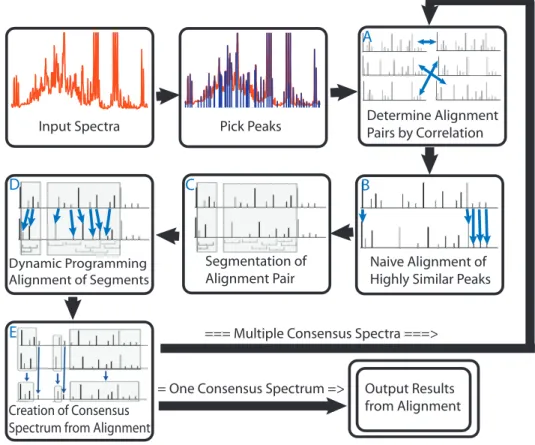
Figure 2.1: Overview of the PCANS Alignment Process. The alignment process loops through multiple iterations of pairwise alignment until achieving a single consensus profile. See text for further details.

at peak apex, chemical shift position at peak apex, and the width at half-height of the peak.

The width at half-height is calculated by fitting a triangle to the peak based on the points

prior and immediately after the apex point. The base of the triangle estimates the width at half

height for the peak. The peaks from NMR spectra are not perfect Lorentzians because multiple

compounds compose a sample; therefore, relative intensity (height) and width at half-height are not redundant information.

The overall flow of the PCANS alignment algorithm is diagrammed in Figure 2.1. Detailed

algorithm pseudocode for both naive and dynamic programming alignment is provided in the

next section . After peak detection, the remaining alignment steps are the same for both

real and simulated spectra. The process begins with highly similar pairs of spectra being

(28)

We note that the statistical correlation between spectra will be more influenced by the larger

peaks, but this is simply a starting point in choosing which spectra to try and align first into a consensus spectrum; all peaks will ultimately be aligned. Once the alignment pairs have been

identified, the pairwise alignment process begins with naive peak alignment as illustrated in

Figure 2.1B. The naive peak alignment algorithm aligns corresponding peaks within the pair

that have ninety percent or greater similarity across all peak attributes. Doing so also generates

unaligned regions that are often bounded on both sides by regions composed solely of these

highly similar (and easily alignable) peaks.

In both the naive as well as dynamic programing alignment, described next, crossover of

peaks is prevented. Here, crossover is defined as shifting a peak over an adjacent peak that has already been aligned to a peak in the paired peak profile. In addition, peaks are restricted

by the amount of chemical shift position movement that is allowed based upon a user defined

maximum. Therefore, a pair of peaks will only align together if the amount of movement that

the peaks need to make for the alignment is less than this user defined maximum. Typically,

the user would define this maximum chemical shift position movement as ±0.04 or ±0.03 ppm, but the value is data dependent. We note that by aligning each peak within its own user

defined window the notion of linear or non-linear shifting of peaks across the spectrum need not be considered.

The next step in alignment involves defining corresponding unaligned segments of the

peak profile pair as depicted in panel C of Figure 2.1. Here, each spectra is segmented such

that only the unaligned peaks contained within a segment will be subject to the dynamic

programming alignment process. Again, these segments are paired between the two peak

profiles and segments are bounded on each side either by already aligned regions or “empty”

regions where it is impossible to form an alignment between a pair of peaks based upon the user-defined maximum chemical shift variation.

Both the naive and dynamic programming alignment schemes rely upon a scoring function

(29)

this similarity score is different from correlation, despite it ranging from 0.0 to 1.0. This

score indicates the proportion of similarity between two peaks, i.e. a score of 1.0 indicates the corresponding peaks are exactly the same. The similarity is determined based on the three

peak attributes of height at apex, h, width at half height, w, and chemical shift position, c. While in this work each of the three peak attributes are assigned so as to contribute an equal

proportion to the score, the assignment of these proportions, ph, pw and pc can readily be

altered as appropriate. For both height and width, the similarity is measured by difference

of the two values scaled by the larger of the two subtracted from one. For the variation in

chemical shift, the similarity is measure by the difference scaled by the user defined maximum

amount of acceptable variation between peaks,m, subtracted from one.

Score = ph∗

1− ha−hb max(ha,hb)

+ pw ∗

1− wa−wb max(wa,wb)

+ pc∗

max1−ca−cb m

,0 (2.1)

A modified dynamic programming algorithm is used to align peaks within each of the

segments (see next section for pseudocode). The algorithm involves using the typical dynamic

programming recursion, where the scores assigned for a given alignment between peaks are

defined using the scoring function enumerated above with a gap penalty, gp, is imposed for unaligned peaks. The modification involves assigning a large penalty, the boundary penalty bp, when alignment between two peaks involves chemical shift variation greater than m or when two aligned peaks do not achieve the minimum acceptable similarity for alignment,

minScr. The user defines both of these values, -0.10gp and -5.0bp in this work, with the assignment of the large penalty preventing the algorithm from violating either the maximum

(30)

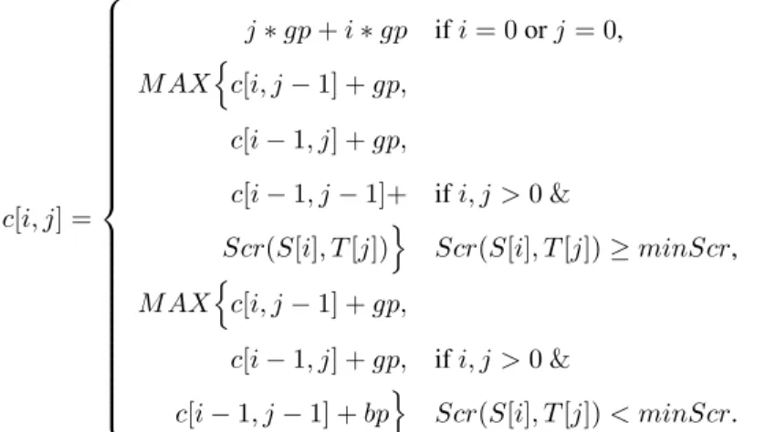
programming scheme is the following (Equation 2.2). Given a pair of spectra S andT, one defines a scores matrixcsuch thatchasirows equal to length(S) + 1 andj columns equal to length(T) + 1. The functionScr(x, y)returns the similarity score between two peaks, x and y, computed using the formula above. The gap penalty,gp, should be greater in value than the boundary penalty, bp. The gap penalty can range from the user defined minimum similarity, minScr(0.60 in this work), to a small negative number, typically -1.0. The boundary penalty should be a large negative number (we used -999 in our implementation to allow the algorithm

to automatically assign its value).

c[i, j] =

                                            

j∗gp+i∗gp ifi= 0orj= 0,

M AXnc[i, j−1] +gp,

c[i−1, j] +gp,

c[i−1, j−1]+ ifi, j >0 &

Scr(S[i], T[j])o Scr(S[i], T[j])≥minScr,

M AXnc[i, j−1] +gp,

c[i−1, j] +gp, ifi, j >0 &

c[i−1, j−1] +bpo Scr(S[i], T[j])< minScr.

(2.2)

Panel E of Figure 2.1 illustrates the final step in the process where the consensus peak

pro-file is formed. Specifically, the consensus propro-file is generated by assigning a new consensus

peak to each successfully aligned pair of peaks, where this consensus peak takes on the

me-dian chemical shift value and the average relative height and width of the paired aligned peaks. Peaks from either profile that fail to align are allowed to ”pass-through” to the consensus

pro-file and maintain their original attributes. Panel E of Figure 2.1 depicts successfully aligned

peaks as those contained within a shaded box, those that failed alignment are unadorned.

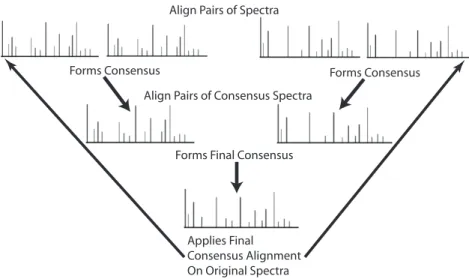
Figure 2.2 illustrates how the entire process diagrammed in Figure 2.1 is repeated on the

resulting consensus profiles until a single consensus profile is produced. The peak profiles

in the top row of figure 2.2 demonstrate the initial step where the pairs of input profiles are

(31)

Align Pairs of Spectra

Forms Consensus Forms Consensus

Align Pairs of Consensus Spectra

Forms Final Consensus

Applies Final Consensus Alignment On Original Spectra

Figure 2.2: Final Consensus Profile Formation. Pairwise alignments are progressively com-bined together through the alignment of consensus profiles to form a final consensus profile. This profile is then used to adjust the chemical shift positions of the peaks from the original input peak profiles to their final aligned positions.

is repeated until only a single consensus profile exists as depicted at the bottom of Figure 2.2.

This final consensus profile is used to adjust the chemical shift positions of the peaks from the

original input profiles to their final aligned positions.

For the determination of optimal alignment parameters (ph,pw andpcin the scoring

func-tion), we perturbed the peak attributes of the simulated peak profiles in a variety of different

ways. Figure 2.3 depicts a representative result of one of the many simulations that were run. The results from these experiments indicate that using equal proportions is robust regardless

of the perturbations introduced, as long as all three attributes experienced some amount of

per-turbation. If the amount of perturbation experienced by one of the three attributes is expected

to be considerably less than the other two, the user might consider increasing its contribution

to the score function.

2.2.4 Alignment Algorithms

(32)

Chemical Shift Contribution to Score

.40/.60 .45/.55 .50/.50 .55/.45 .60/.40

0.250 0.333 0.400 0.450 0.500

0.890 0.895 0.900 0.905 0.910

Height/Width Contribution to Score

.40/.60 .45/.55 .50/.50 .55/.45 .60/.40

0.250 0.333 0.400 0.450 0.500

0.024 0.026 0.028 0.030 0.032 0.034 A

B

(33)

the number of peaks that were picked for peak profileX. The inputs for the pseudocode below involve only aligning a pair of peak profiles, S and T, such that S, T ∈ A, {i | A[S, i],1 ≤ i≤nS}and{j |A[T, j],1≤j ≤nT}.

2.2.5 Naive Alignment Scheme

The naive alignment incorporates a greedy algorithm that will align two nearby peaks as

long as they are close in proximity (chemical shift position) to each other and achieve a

high similarity score (i.e. also have high similarity in height and width). The procedure

N aiveAlign(S,T,maxCS,minScoreN), naively aligns the pair of peak profiles S and T. This procedure inputsmaxCS, the chemical shift value that is the maximum the user expects to have to shift a peak to obtain a match, andminScoreN, the minimum value of the similar-ity between two peaks to allow for naive alignment. Additionally, the value ofminScoreN is used to define the required amount of similarity in chemical shift position that two peaks must

have to allow naive alignment.

The similarity between two peaks is calculated using the function CalcScore(S[i], T[j], maxCS)which is based on the similarity score formula presented in the methods section of the paper. Typically,minScoreN should be a high value of 0.88 or greater (0.90 for this pa-per) andmaxCS should range within 0.04 - 0.02 ppm (0.04 for this paper). Naive alignments are made using the procedure M akeN aiveM atch(S,T,sIdx,tIdx), which is not illustrated below due to its reliance on our algorithm’s spectra data structure. TheM akeN aiveM atch procedure makes the naive matches given the input pair of peak profiles and the indices of

their peaks that match. Nothing is returned, but the underlying peak profile data structure is

changed to reflect the naive matches. Pseudocode for the algorithm can be found below as

Algorithm 1 for naive alignment with the two helper functions defined in Algorithm 2 and

(34)

Algorithm 1

NaiveAlign(S, T, maxCS, minScoreN) ≡

m←length[S] ssT ←1

searchCS ←maxCS ∗(1.0−minScoreN)

fori←1tomdo

temp←ReturnStart(S, T, searchCS, i, ssT)

iftemp6=−999

thenssT ←temp

matchI ←ReturnM axM atchIdx(S, T, maxCS, searchCS, i, ssT, minScoreN)

ifmatchI 6=−999

thenM akeN aiveM atch(S, T, i, matchI)

fi fi

(35)

Algorithm 2

ReturnStart(S, T, searchCS, idxS, ssT) ≡

n←length[T] z ←ssT

ifT[z].chemShif t≥(S[idxS].chemShif t−searchCS)

then

while(z >1andT[z].chemShif t >(S[idxS].chemShif t−searchCS))do

z ←z−1

end

if(z ≥1andT[z].chemShif t≤(S[idxS].chemShif t−searchCS))

then ifT[z].chemShif t= (S[idxS].chemShif t−searchCS)

thenrssT ←z

elserssT ←z+ 1

fi

elserssT ← −999

fi else

while(z < nandT[z].chemShif t <(S[idxS].chemShif t+searchCS))do

z ←z+ 1

end

if(z ≤nandT[z].chemShif t≥(S[idxS].chemShif t+searchCS))

then ifT[z].chemShif t= (S[idxS].chemShif t+searchCS)

thenrssT ←z

elserssT ←z−1

fi

elserssT ← −999

fi fi

(36)

Algorithm 3

ReturnMaxMatchIdx(S, T, maxCS, searchCS, idxS, ssT, minScoreN) ≡

n←length[T] z ←ssT

bestV ←CalcScore(S[idxS], T[z]) bestI ←z

z ←z+ 1

while(z ≤nandT[z].chemShif t≤(S[idxS].chemShif t+searchCS))do

ifbestV < CalcScore(S[idxS], T[z], maxCS)

thenbestV ←CalcScore(S[idxS], T[z], maxCS) bestI ←z

fi

z ←z+ 1

end

ifbestV < minScoreN

thenbestI ← −999

fi

returnbestI

2.2.6 Dynamic Programming Alignment Scheme

To dynamically align the pair of peak profilesS andT, the procedureDynP rogAlign(S,T, maxCS,gp,bp,minScoreD) uses the recursive formula defined in the methods section of the paper. The recursive formula from the paper defines an alignment scores matrix c[i, j] and the backtrack matrixb[i, j]that indicate the optimal solution. Notice that indicesiandjfrom these matrices (scores and backtrack) are defined asi=0,...,nSandj=0,...,nT. The pseudocode

in Algorithm 4 follows a modified dynamic programming alignment scheme as outlined by

the recursive formula in the paper.

(37)

align-ment, minScoreD, or if two peaks’ difference in chemical shift position is greater than the maximum allowable chemical shift variation, maxCS. The gap penalty, gp, and boundary penalty,bp, can be input by the user.

Typically,minScoreDis a high value of 0.50 or greater, but this parameter should be set based upon the user’s discretion (for this paper 0.60). The gap penalty (-0.10 for this paper)

should be greater in value than the boundary penalty (-5.0 for this paper). The gap penalty can

range from the user defined minimum similarity, minScoreD, to a small negative number, typically -1.0. The boundary penalty should be a large negative number or set to -999 to allow

the algorithm to automatically set the value. Pseudocode for the algorithm can be found below

as Algorithm 4. Notice for simplicity theCalcScore(S[i], T[j], maxCS, minScoreD) func-tion in the algorithm is implemented in a manner that returns a similarity score that is less than

(38)

Algorithm 4

DynProgAlign(S, T, maxCS, gp, bp, minScoreD) ≡

m←length[S] n←length[T]

ifbp ==−999

thenbp=gp∗n∗m

fi

fori←0tomdo

forj ←0tondo

ifi= 0orj = 0

thenc[i, j]←i∗gp+j ∗gp

ifi= 0

thenb[i, j]←”←”

elseb[i, j]←”↑”

fi

elseDiagScore←CalcScore(S[i], T[j], maxCS, minScoreD)

ifDiagScore < minScoreD

thenDiagScore←bp

fi

if(c[i−1, j−1] +DiagScore≥c[i−1, j] +gp)and (c[i−1, j−1] +DiagScore≥c[i, j−1] +gp)

thenc[i, j]←c[i−1, j−1] +DiagScore b[i, j]←”-”

if else(c[i−1, j] +gp≥c[i−1, j−1] +DiagScore)and

(c[i−1, j] +gp≥c[i, j−1] +gp)

thenc[i, j]←c[i−1, j] +gp b[i, j]←”↑”

elsec[i, j]←c[i, j−1] +gp b[i, j]←”←”

fi fi

fi end end

2.2.7 Algorithm speed

In our Python implementation, alignment of the described 22 real mouse urine spectra takes

approximately 2 minutes on a 2GHz laptop. Approximately 30 seconds involves the actual

(39)

process-ing. Alignment of 150 real mouse urine spectra takes approximately 38 minutes with 1 min

54 sec being involved in alignment.

2.2.8 Simulation of NMR spectra peak profiles

To generate NMR profiles that were as realistic as possible our simulated peak profiles are

based upon characteristics of urine spectra from mice. Specifically, we follow the distribution

of peak locations, heights and widths as estimated from murine urine spectra using the

spec-trum visualization utility implemented in ACD 1D NMR Processor, version 11 (Advanced

Chemistry Development, Toronto, Canada). The spectral peaks used for calculating these

dis-tributions range in chemical shift position from 2.0 ppm to 4.10 ppm. These disdis-tributions are

coded into a software utility that allows the generation of simulated peak profiles. In addition, user-defined levels of noise in chemical shift position, height and width can be defined. To

help simulate attributes observed with real NMR spectra, the number of peaks generated per

spectrum is varied through the addition of noise peaks to the simulated profiles. To evaluate

algorithm performance with profiles originating from multiple distinct classes, we generate

spectra from distinctly different templates where the user defines the number of peaks

com-mon between templates.

2.3 Results

While the alignment method we propose consists of several steps which are described in detail

in Methods, we provide a brief overview here. As outlined in Figure 2.1, our approach begins by first characterizing each individual spectrum by defining its peaks. The process of picking

peaks can be done through a variety of methods and we have used a straightforward approach

that uses the derivative of the spectrum, and other associated properties for discerning peaks.

The resulting set of peaks contains the location, height and width of all peaks in a spectrum,

(40)

used in the interpretation of NMR spectra. This approach allows each NMR spectrum to be

represented by a much smaller collection of data points than if we used the full resolution of the acquired spectrum. For example, our experimental urine spectra were collected with

16384 points, but the peak picking process found that the spectrum contained less than 500

significant peaks. It must be noted that peak picking may result in loss of information if some

peaks are not picked. The peak picking algorithm is under active development to ensure that

peak information is not lost due to features such as low signal to noise or spectral crowding.

Future work will also consider spectral features such as multiplet structure to provide more

accurate peak profiles.

In the next step of the process, pairs of peak profiles are chosen for alignment, where the most similar profiles are determined through pair-wise statistical correlation (Figure 2.1A).

Thus we start by aligning the most similar pairs of profiles to each other first. Each of these

pairs of profiles is then aligned through a series of progressively more rigorous steps that

be-gins with the naive alignment of the most highly similar peaks (Figure 2.1B-D). This naive

alignment establishes aligned regions of high identity separated by segments that cannot be

so readily aligned. These segments, bordered on either side by high-confidence aligned

re-gions, are then aligned through a dynamic programming algorithm where the alignment score is based on chemical shift position, peak height and peak width. Note that only the peak

location is altered throughout the alignment process and that peak height and width remain

unaltered. Following this first pairwise alignment, a single consensus profile is created (Figure

2.1E). This process is then repeated, first for each set of pairs and then progressively for all

of the generated consensus profiles. At the end of this process a single representative

consen-sus profile is generated which defines the final alignment (see Figure 2.2). The final output

(41)

2.3.1 Alignment of simulated spectra

As ”gold-standard” completely characterized NMR spectra for use in validation are not

avail-able, we used a simulation approach for generating peak profiles that could then be used to assess the performance of the alignment methods. In particular, the use of simulated profiles

allows us to determine whether or not two or more peaks aligned through our algorithm should

actually be aligned with each other, and if not, which other peaks they should be aligned to.

It also allows us to introduce defined amounts of noise, either in the form of chemical shift

variation, peak height, peak width, or randomly introduced ”noise” peaks into each profile

and measure their effect on alignment accuracy. As we wished to generate NMR profiles that

were as realistic as possible, our simulated profiles were composed of a subset of peaks picked from an actual mouse urine spectrum (see Methods).

As a test of our alignment approach, we attempted to align simulated profiles under a

vari-ety of noise conditions. In these tests we generated two sets of profiles consisting of 32 profiles

each, where each set was based on a different template. Each template consisted of a total of

50 peaks, 13 of which were unique to each group, allowing us to look at the effectiveness of

alignment in the presence of inter-group variation. In addition to the differences derived from

the peaks specific to each group, predefined amounts of chemical shift, peak height and peak

width variation were also introduced before alignment. Finally, 50% of the profiles in each group had from 1 to 4 additional noise peaks inserted at random positions within each profile.

The effects of chemical shift variation on alignment accuracy are shown in Figure 2.4

where, in addition to chemical shift variation, 25% of peaks were subject to noise of±10% in peak height and/or peak width at half-height. The contribution of chemical shift, peak height

and width to the alignment score were kept equal in this and all other tests as this combination

was found to be highly robust. Sensitivity to the choice of these weighting parameters is shown

in 2.3. In Figure 2.4 we see that the accuracy of alignment is highly robust to chemical shift variation as can be seen by the slow decrease in accuracy with increasing variation. Here,

(42)

+/− Chemical Shift Variation from Origin

Proportion of Peaks with Chemical Shift Variation

0.010 0.015 0.020 0.025 0.030 0.035 0.040 0.10

0.20 0.30 0.40 0.50

0.89 0.91 0.92 0.93 0.94 0.95 0.96 0.97 0.98

(43)

+/− Chemical Shift Variation from Origin

Proportion of Peaks with Chemical Shift Variation

0.010 0.015 0.020 0.025 0.030 0.035 0.040 0.10

0.20 0.30 0.40 0.50

0.015 0.020 0.025 0.030

(44)

total number of peaks. Alignment is similarly robust to increases in the proportion of peaks

subjected to such variation. In fact, a nearly 90% accuracy is maintained despite 50% of peaks experiencing variation of up to±0.04ppm. The maximum standard deviation is±0.033and the corresponding map of deviations is shown in Figure 2.5. While we used a window of ±0.04ppm in the alignment of individual peaks, this is a user-defined quantity that can be

changed to suit the underlying data.

We also compared the accuracy of our alignment method between our consensus approach

and the use of a template. Again, we started with two sets of profiles, with each set consisting

of 32 profiles and 50 peaks, with 13 peaks unique to the set. Variation in chemical shift

position (±0.02 ppm) was introduced for 50% of the peaks. Peak height and width noise (25% of peaks affected with±10%variation) was also independently introduced. As before, 50% of the profiles in each group had 1 to 4 noise peaks inserted at random chemical shift

positions.

We iteratively chose one of the sixty-four peak profiles as the template to which all the

other profiles were aligned. Thus this approach differs from the PCANS alignment method

only in the fact that it uses a representative profile as a template for use in aligning the other

peak profiles; all other steps are identical including the dynamic programming alignment of peaks. Over all 64 possible templates, the average accuracy using this approach was 84.4%

with 99% confidence intervals of 84.02% and 84.68%. The best single template had an

accu-racy of 87.5%. In contrast, PCANS had a 93.9% accuaccu-racy (PCANS generates only one answer

so there are no error bars in this case).

A representative region of an alignment is shown in Figure 2.6 where the template

gener-ating the highest accuracy (87.5%) was used to generate the shown template-based alignment.

Differences between the template, unaligned and PCANS alignments can be readily observed. For example, three regions are highlighted that have peaks unique to Group 1. In Region 1 of

the unaligned spectra (center row), it is possible to pick out by eye the existence of two likely

(45)

3.78 3.83 3.89 3.94 3.99 4.05 4.11 10 20 30 40 50 60 Spectra 3.78 3.83 3.89 3.94 4.00 4.05 4.11 10 20 30 40 50 60

Chemical Shift3.94 3.89 3.83 3.78

4.00 4.05 4.11 10 20 30 40 50 60 2.39 4.78 7.16 9.55 11.94 14.33 Template Align Unaligned PCANS Group 1 Group 2 Group 2 Group 2 Group 1 Group 1

Region 1 Region 2 _{Region 3}

(46)

to Group 2 is also visible in this region. In the template alignment (top row) the two peaks of

Group 1 could not be aligned, as the best overall template did not contain associated peaks in these locations. In addition, the template did have a peak in Group 2, but at the wrong

loca-tion, forcing alignment of the unique Group 2 peak to a shifted location. In contrast, PCANS

correctly aligned the Group 2 peak (bottom row). Furthermore, the two peaks unique to Group

1 were also successfully aligned. Note that the rightmost peak of the pair appears to be shifted

to the right. This is due to the variation present within the unaligned set of peaks. Aligning

noisy spectra containing peaks with varying chemical shift position with PCANS results in the

alignment of peaks at their median chemical shift position. This provides a robust estimate of

peak position despite potentially significant amounts of spectral noise.

In Region 2 of the template alignment, we see a well-aligned peak for Group 1. However,

as we are using simulated data, we know that the position of this alignment is centered at a

nearby noise peak within the template profile and inspection of the unaligned profiles also

shows no obvious peak. The correct result is shown in Region 2 of the PCANS alignment.

This incorrect alignment occurs because the “best” template happens to contain a nearby noise

peak that is used as the basis for alignment of all other profiles.

Finally, in Region 3 (unaligned) we see strong indications of a peak in Group 1 as well as alignment of this peak with PCANS. However, in the template alignment we see no obvious

change relative to the unaligned profiles. This is due to the fact that the template profile had no

peaks in this region and thus none of the identified peaks could be aligned. The fact that they

are present at all in the final alignment is due to the PCANS-portion of the algorithm

(non-template), which allows these orphan peaks to pass through to the final alignment regardless of

whether or not they are found in the template. Overall, this example demonstrates the inherent

(47)

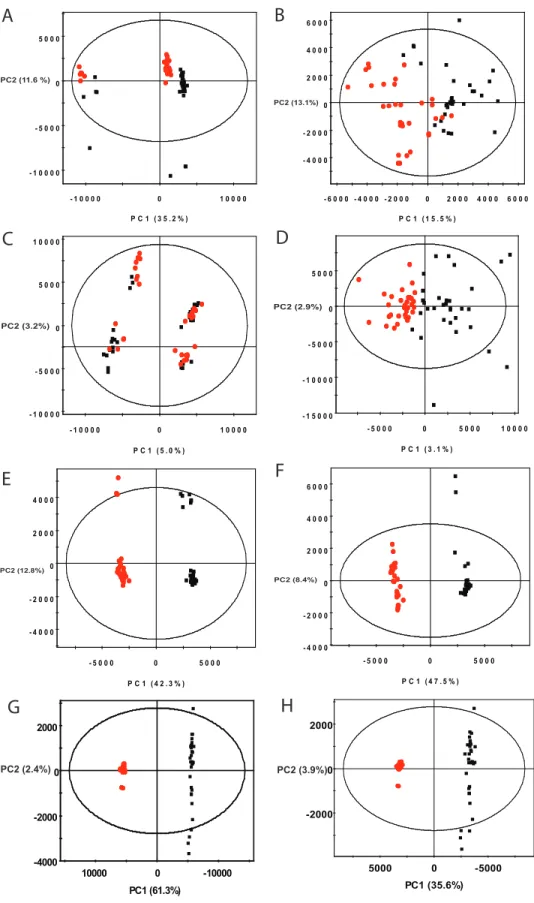
- 1 0 0 0 0 - 5 0 0 0 0 5 0 0 0

- 1 0 0 0 0 0 1 0 0 0 0 PC2 (11.6%)

P C 1 ( 3 5 . 2 % ) SIMC A-P+ 12 - 2009-02-11 04:41:35 (U TC -5) PC2 (11.6 %)

- 4 0 0 0 - 2 0 0 0 0 2 0 0 0 4 0 0 0 6 0 0 0

- 6 0 0 0 - 4 0 0 0 - 2 0 0 0 0 2 0 0 0 4 0 0 0 6 0 0 0 PC2 (13.1%)

P C 1 ( 1 5 . 5 % ) SIMC A-P+ 12 - 2009-02-16 14:58:31 (U TC -5) PC2 (13.1%)

- 1 0 0 0 0 - 5 0 0 0 0 5 0 0 0 1 0 0 0 0

- 1 0 0 0 0 0 1 0 0 0 0 PC2 (3.2%)

P C 1 ( 5 . 0 % ) SIMC A-P+ 12 - 2009-02-16 15:00:09 (U TC -5)

- 1 5 0 0 0 - 1 0 0 0 0 - 5 0 0 0 0 5 0 0 0

- 5 0 0 0 0 5 0 0 0 1 0 0 0 0 PC2 (2.9%)

P C 1 ( 3 . 1 % ) SIMC A-P+ 12 - 2009-02-16 15:01:25 (U TC -5)

- 4 0 0 0 - 2 0 0 0 0 2 0 0 0 4 0 0 0

- 5 0 0 0 0 5 0 0 0 PC2 (12.8%)

P C 1 ( 4 2 . 3 % ) SIMC A-P+ 12 - 2009-02-16 15:02:52 (U TC -5)

- 4 0 0 0 - 2 0 0 0 0 2 0 0 0 4 0 0 0 6 0 0 0

- 5 0 0 0 0 5 0 0 0 PC2 (8.4%)

P C 1 ( 4 7 . 5 % ) SIMC A-P+ 12 - 2009-02-16 15:04:02 (U TC -5)

C

D

B

A

E

F

PC2 (8.4%) PC2 (12.8%) PC2 (2.9%) PC2 (3.2%) -4000 -2000 0 2000 -10000 0 10000 adfsafdPC2 (2.4%) PC1 (61.3%) PC2 (2.4%) -2000 0 2000 -5000 0 5000 PC2 (3.9%) PC1 (35.6%) SI MC A-P+ 12 - 2009-10-27 15:40: 43 (U TC -5) PC2 (3.9%)

4898.pdf

Systematic approaches to integrate inconsistent, noisy

high-throughput data to bolster subtle relationships

obscured by standard analyses

Abstract

Acknowledgments

Table of Contents

List of Tables

List of Figures

Chapter 1

Introduction

1.1

Motivation and Goals

1.2

Brief Overview of Existing Methods

1.2.1

NMR Spectra Noise Reduction Methods

1.2.2

Identifying Association in Inconsistent, Noisy Data

1.3

Approach and Innovations

1.3.1

Methods to Enhance NMR Spectra Analysis

1.3.2

Methods to Enhance Association Identification

1.3.3

Thesis

1.3.4

Contributions to Enhance NMR Spectra Analysis

1.3.5

Contributions to Enhance Association Identification

1.4

Dissertation Outline

Chapter 2

Enhancing Metabolomic Analysis with PCANS

2.1

Background

2.2

Methodology

2.2.1

Experimental NMR data collection and processing

2.2.2

Multivariate statistical analysis

2.2.3

Peak picking

2.2.4

Alignment Algorithms

2.2.5

Naive Alignment Scheme

2.2.6

Dynamic Programming Alignment Scheme

2.2.7

Algorithm speed

2.2.8

Simulation of NMR spectra peak profiles

2.3

Results

2.3.1

Alignment of simulated spectra

C

D

B

A

E

F

G

H