The handle http://hdl.handle.net/1887/46454 holds various files of this Leiden University
dissertation
Author: Pas, S.L. van der
Proefschrift
ter verkrijging van
de graad van Doctor aan de Universiteit Leiden,
op gezag van Rector Magnificus prof. mr. C.J.J.M. Stolker,
volgens besluit van het College voor Promoties
te verdedigen op dinsdag 28 februari 2017
klokke 11.15 uur
door
Promotor: prof. dr. A.W. van der Vaart Universiteit Leiden
Promotiecommissie: prof. dr. I. Castillo Université Paris VI prof. dr. R.D. Gill Universiteit Leiden
prof. dr. P.D. Grünwald Universiteit Leiden (secretaris) dr. S. Gugushvili Universiteit Leiden
dr. V. Ro˘cková University of Chicago
Research supported by the Netherlands Organization for Scientific Research (NWO).
List of papers v
Introduction 1
1 Posterior concentration of the horseshoe around nearly black vectors 7
1.1 Introduction . . . 8
1.2 The horseshoe prior . . . 9
1.3 Mean square error and bounds on the posterior variance . . . 12
1.4 Empirical Bayes estimation ofτ . . . 14
1.5 Simulation study . . . 16
1.6 Concluding remarks . . . 18
1.7 Proofs . . . 19
2 Conditions for posterior concentration for scale mixtures of normals 39 2.1 Introduction . . . 40
2.2 Main results . . . 41
2.3 Examples . . . 48
2.4 Simulation study . . . 53
2.5 Discussion . . . 55
2.6 Proofs . . . 55
3 Adaptive inference and uncertainty quantification for the horseshoe 63 3.1 Introduction . . . 64
3.2 Maximum marginal likelihood estimator . . . 68
3.3 Contraction rates . . . 69
3.4 Coverage . . . 72
3.5 Simulation study . . . 79
3.6 Proofs . . . 84
4 Bayesian community detection 117 4.1 Introduction . . . 117
4.2 The stochastic block model . . . 119
4.3 Bayesian approach to community detection . . . 121
4.4 Application to the karate club data set . . . 125
4.5 Discussion . . . 127
4.6 Proofs . . . 128
5 The switch criterion in nested model selection 143 5.1 Introduction . . . 143
5.2 Model selection by switching . . . 147
5.3 Rate-optimality of post-model selection estimators . . . 149
5.4 Main result . . . 153
5.5 Robust null hypothesis tests . . . 157
5.6 Discussion and future work . . . 162
5.7 Proofs . . . 166
6 Bilateral patients in arthroplasty registry data 183 6.1 Introduction . . . 183
6.2 Competing risk of death . . . 184
6.3 Dependence between hips and the time-dependent bilateral status . . . 187
6.4 Data structure . . . 195
6.5 Results on the LROI data . . . 198
Bibliography 213
Samenvatting 225
Dankwoord 227
The first five chapters of this thesis consist of the papers listed below, with minor changes to the references.
Chapter 1:
van der Pas, S.L., Kleijn, B.J.K. and van der Vaart, A.W. (2014), The horseshoe estima-tor: posterior concentration around nearly black vectors,Electronic Journal of Statistics8,
2585–2618.
Chapter 2:
van der Pas, S.L., Salomond, J.-B. and Schmidt-Hieber, J. (2016), Conditions for posterior contraction in the sparse normal means problem,Electronic Journal of Statistics10, 976–
1000.
Chapter 3:
van der Pas, S., Szabó B. and van der Vaart, A., How many needles in the haystack? Adap-tive inference and uncertainty quantification for the horseshoe.Submitted.
Chapter 4:
van der Pas, S.L. and van der Vaart, A.W., Bayesian community detection.Submitted.
Chapter 5:
van der Pas, S. and Grünwald, P., Almost the best of three worlds: risk, consistency and optional stopping for the switch criterion in nested model selection. To appear inStatistica Sinica.
The sixth chapter is based on material from the following two unpublished papers.
Chapter 6:
van der Pas, S.L., Nelissen, R.G.H.H. and Fiocco, M., Staged bilateral total joint arthroplasty patients in registries. Immortal time bias and methodological options.Submitted.
van der Pas, S.L., Nelissen, R.G.H.H., Schreurs, B.W. and Fiocco, M., Risk factors for early revision after unilateral and staged bilateral total hip replacement in the Dutch Arthro-plasty Register.In preparation.
This thesis is composed of papers on four topics: Bayesian theory for the sparse nor-mal means problem (Chapters 1-3), Bayesian theory for community detection (Chapter 4), nested model selection (Chapter 5), and the application of competing risk methods in the presence of time-dependent clustering (Chapter 6). Each topic is briefly introduced in this Introduction.
Sparsity and shrinkage priors (Ch. 1 - 3)
A problem is sparse when there are only a few signals amidst a lot of noise. Those signals are like the proverbial needles in a haystack. The field of astronomy contributes many examples, such as supernovae detection (Clements et al., 2012). Other examples include the detection of genes associated to a certain disease (Silver et al., 2012) and image com-pression (Lewis and Knowles, 1992).
The particular sparse problem studied in the first three chapters of this thesis is the sparse normal means problem, also known as the sequence model. In the sparse normal means problem, a vectorYn ∈Rn,Yn =(Y1,Y2, . . . ,Yn), is observed, and assumed to have
been generated according to the following model:
Yi =θi +εi, i=1, . . . ,n,
where theεi are assumed to be i.i.d. normally distributed with mean zero and known
varianceσ2, and the vector of meansθ ∈ Rn is the parameter of interest. The sparsity
assumption takes the form of assuming thatθ isnearly black, meaning that almost all
of its entries are zero. The number of nonzero entries inθ is denoted bypn, a number
which is assumed to increase withn, but not as fast asn: pn → ∞,pn = o(n). Other
sparsity assumptions are possible, such as assuming thatθis in a strong or weak`s-ball
fors ∈(0,2)(Castillo and Van der Vaart, 2012; Johnstone and Silverman, 2004), but we do
not pursue these further here.
The inferential goal can take several forms.Recoveryof the parameterθis one possible
goal, and this is the main focus of Chapters 1 and 2.Uncertainty quantificationis a second,
and this is the topic of Chapter 3. A third goal, model selection, is not explored in this
thesis, although the results in Chapter 3 do provide some avenues for further research. There are many ways to achieve the aforementioned goals. The contributions of this thesis are in the field of frequentist Bayesian theory. The parameter of interest is equipped
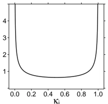
κi 1
2 3 4
0.0 0.2 0.4 0.6 0.8 1.0
Figure 1: Prior density ofκi forτ =1.
with a prior, which, when combined with the likelihood, leads to a posterior distribution, aspects of which we use to achieve our goals. We study the properties of the posterior from a frequentist point of view, meaning that we assume that there is some underlying true parameter that is generating the data.
The priors proposed for the sparse normal means problem are in general shrinkage priors, designed to yield many estimates close to or exactly equal to zero. The particular shrinkage prior studied in this thesis is thehorseshoe prior(Carvalho et al., 2010). It has
become popular, due to its good behaviour in simulation studies, and favorable theoretical properties (e.g. Armagan et al. (2013); Bhattacharya et al. (2014); Carvalho et al. (2010); Polson and Scott (2012a)). It has intuitive appeal, which can be explained through the
origin of its name. The horseshoe prior is given by
θi |λi,τ ∼ N(0,σ2τ2λ2i), λi ∼C+(0,1),
fori =1, . . . ,n, whereC+(0,1) is the standard half-Cauchy distribution. The parameter τ is a global parameter, shared by all means, while the parameterλi is a local parameter.
Howτshould be set is one of the main topics of Chapters 1 and 3. Regarding the name, if τis known, we have the equality:
E[θi |Yi =yi,τ]=(1−E[κi |Yi =yi,τ])yi,
whereκi =(1+τ2λ2i)−1, andE[κ
i |Yi =yi] can be interpreted as the amount of shrinkage
towards zero. A half-Cauchy prior onλi implies a Be(12,12) prior onκiin the special case
whenτ = 1. The horseshoe prior is named after the Be(12,12) prior, which resembles a
horseshoe (Figure 1).
The intuitive appeal lies in the concentration of mass near zero and one, which caters to the true signals and the nonzero means respectively. Decreasingτ leads to more prior
mass near one, corresponding to more shrinkage. One of the main contributions of this thesis is the guideline that optimal recovery (in the minimax sense) can be achieved by settingτ at most of the order(pn/n)plog(n/pn)(Chapter 1).
In practice, the numberpn is unknown and thus there is a need for a procedure that
The first is empirical Bayes, whereτis estimated based on the data and the resulting value
plugged into the prior. The second is hierarchical Bayes, whereτ receives a hyperprior.
In both cases, recovery ofθ is possible at the near-minimax rate, and credible balls are
both honest (they contain the true value with some prescribed probability) and adaptive (they are as small as possible), under some conditions. In addition, credible intervals are guaranteed to have good coverage if the underlying signal is either ‘small’ or ‘large’, but almost surely do not contain the truth if the signal is close to approximatelyp
2 logn.
The results of Chapter 1 led to the question what properties of the horseshoe prior make it so well suited for recovery, and whether it is unique in that regard. The results from Chapter 2 show that the horseshoe is not that special: many priors in the class of scale mixtures of normals enjoy the same good behaviour. We provide conditions under which the posterior contracts at the minimax rate. Recovery of the nonzeroes requires tails that are at least exponential; recovery of the zeroes requires sufficient mass close to zero, and not too much mass in the interval [(pn/n)log(n/pn),1]. Many priors satisfy
these conditions. However, the horseshoe may be special after all, because it represents a boundary case with respect to the thickness of its tails. This could explain the good cov-erage properties of the horseshoe’s credible balls. Whether the uncertainty quantification properties of the horseshoe, as described in Chapter 3, can be generalized to scale mixtures of normals is an open question.
An attractive property of the horseshoe is that some of the aspects of its posterior can be easily and quickly computed, without the need for MCMC. Functions for the horse-shoe’s posterior mean, posterior variance, the MMLE and credible intervals are available in the R package ‘horseshoe’ (van der Pas et al., 2016).
Community detection (Ch. 4)
In this chapter, like the previous ones, Bayesian posterior distributions are studied from a frequentist point of view, but unlike the previous chapters, the theory is for data with a network structure. The aim is to detect communities in, for example, a social network. The network is assumed to be generated according to thestochastic block model, in which the
probability of the existence of a connection between two individuals (nodes) only depends on each individual’s community membership.
We equip all parameters of the stochastic block models with priors, and use the poste-rior mode as an estimator of the community memberships (MAP-estimation). We call the resulting estimator theBayesian modularity, following Bickel et al. (2009). Two instances
are studied. In the first, thedensesituation, the probabilities of connections between
in-dividuals remain fixed. The second and most complicated situation is thesparsesituation,
in which the probability of a connection between two individuals tends to zero as the network grows in size.
Weak and strong consistency are proven, the former meaning that only a fraction of the nodes are misclassified, and the latter that none of the nodes are misclassified. The theorems require the assumption that the expected degree is at least of order log2n, where nis the number of nodes in the network. Whether this assumption can be weakened to
Nested model selection (Ch. 5)
In Chapter 5, we turn to model selection. The models under consideration are nested exponential family models. For example, one model could consist of all univariate normal distributions with unknown mean and unknown variance, while the other model only contains the standard normal distribution.
Optimality of a model selection criterion can be defined in many different ways. Three of them are discussed in this Chapter: consistency, minimax rate optimality, and robust-ness to optional stopping. The switch criterion, a new model selection criterion based on the switch distribution introduced by Van Erven et al. (2012), is evaluated on those three properties.
Consistencyguarantees that if the data is actually generated according to one of the
models, then that model will be selected eventually.minimax rate optimalityis a measure
of the accuracy of the parameter estimation step that follows the model selection. mini-max rate optimality and consistency are mutually exclusive properties (Yang, 2005). The main contribution of Chapter 5 is that the switch criterion is consistent while missing the minimax risk by a factor of order log logn, if the criterion is used in combination with
efficient estimators of the parameters.
The third property, robustness to optional stopping, has attracted attention because most standard null hypothesis significance tests which output ap-value, do not have this
property (Armitage et al., 1969; Wagenmakers, 2007). In the classical framework, a re-searcher has to decide the sample size in advance. This guideline is not always adhered to; in a recent survey of psychologists, approximately 55% of participants admitted to decid-ing whether to collect more data after lookdecid-ing at their results to see if they were significant (John et al., 2012). If a criterion is robust to optional stopping, the validity of the results will not be affected by the use of such stopping rules. As discussed in Chapter 5, the switch criterion is robust to optional stopping, if the null hypothesis is a point hypothesis. Thus, the switch criterion comes close to achieving all three desirable properties.
Hip arthroplasty data and bilateral patients (Ch. 6)
The final chapter of this thesis is on the topic of hip arthroplasty registry data, and is of a different character than the preceding ones. It is the result of an ongoing collaboration with Marta Fiocco, Rob Nelissen and Wim Schreurs. The goal is to determine which patient characteristics are associated with time to revision surgery after hip replacement surgery, using the data collected by the LROI (Landelijke Registratie Orthopedische Implantaten / Dutch Arthroplasty Register).
Total hip arthroplasty (THA) is a common procedure in The Netherlands; the LROI registers approximately 28.000 THAs annually, in most cases following an ostheoarthri-tis diagnosis (LROI, 2014). After the primary surgery, there may be a need for revision surgery, which is defined as any change (insertion, replacement, and/or removal) of one or more components of a prosthesis. Revision may be required due to several reasons, such as mechanical loosening, infection and fracture.
prostheses during the postoperative course of their first hip or knee arthroplasty. In 2014, 20% of THAs in The Netherlands concerned the placement of a second prosthesis (LROI, 2014). Bilateral patients have been theorized to have different risks of revision compared to unilateral patients, as the two hips may affect each other regarding loosening (Buchholz et al., 1985). In addition, although the primary diagnosis for surgery may be osteoarthritis, patients with several total joint arthroplasties within a short time period may reflect a different patient population compared to a patient who has only one implant during a, say, five year follow-up.
1
Posterior concentration of the
horseshoe around nearly black
vectors
Abstract
We consider the horseshoe estimator due to Carvalho et al. (2010) for the multivariate normal mean model in the situation that the mean vector is sparse in the nearly black sense. We as-sume the frequentist framework where the data is generated according to a fixed mean vector. We show that if the number of nonzero parameters of the mean vector is known, the horseshoe estimator attains the minimax`2risk, possibly up to a multiplicative constant. We provide conditions under which the horseshoe estimator combined with an empirical Bayes estimate of the number of nonzero means still yields the minimax risk. We furthermore prove an upper bound on the rate of contraction of the posterior distribution around the horseshoe estimator, and a lower bound on the posterior variance. These bounds indicate that the posterior dis-tribution of the horseshoe prior may be more informative than that of other one-component priors, including the Lasso.
This chapter has appeared as S.L. van der Pas, B.J.K. Kleijn and A.W. van der Vaart (2014). The horseshoe estimator: posterior concentration around nearly black vectors.Electronic Journal of Statistics8, 2585–2618. The
research leading to these results has received funding from the European Research Council under ERC Grant Agreement 320637.
1.1
Introduction
We consider the normal means problem, where we observe a vectorY ∈Rn,Y =(Y1, . . . ,
Yn), such that
Yi =θi +εi, i=1, . . . ,n,
for independent normal random variablesεiwith mean zero and varianceσ2. The vector θ = (θ1, . . . ,θn)is assumed to be sparse, in the ‘nearly black’ sense that the number of
nonzero means
pn:=#{i:θi ,0}
iso(n)asn→ ∞. A natural Bayesian approach to recoveringθwould be to induce sparsity
through a ‘spike and slab’ prior (Mitchell and Beauchamp, 1988), which consists of a mix-ture of a Dirac measure at zero and a (heavy-tailed) continuous distribution. Johnstone and Silverman (2004) analyzed an empirical Bayes version of this approach, where the mixing weight is obtained by marginal maximum likelihood. In the frequentist setup that the data are generated according to a fixed mean vector, they showed that the empirical Bayes coordinatewise posterior median attains the minimax rate, in`qnorm,q ∈(0,2], for
mean vectors that are either nearly black or of bounded`pnorm,p ∈ (0,2]. Castillo and
Van der Vaart (2012) analyzed a fully Bayesian version, where the proportion of nonzero coefficients is modelled by a prior distribution. They identified combinations of priors on this proportion and on the nonzero coefficients (the ‘slab’) that yield posterior distribu-tions concentrating around the underlying mean vector at the minimax rate in`qnorm,
q ∈ (0,2], for mean vectors that are nearly black, and in`q norm,q ∈ (0,2) for mean
vectors of bounded weak`pnorm,p ∈(0,q). Other work on empirical Bayes approaches
to the two-group model includes (Efron, 2008; Jiang and Zhang, 2009; Yuan and Lin, 2005). As a full Bayesian approach with a mixture of a Dirac and a continuous component may require exploration of a model space of size 2n, implementation on large datasets
is currently impractical, although Castillo and Van der Vaart (2012) present an algorithm which can compute several aspects of the posterior in polynomial time, provided suffi-cient memory can be allocated. Several authors, including (Armagan et al., 2013; Griffin and Brown, 2010), have proposed one-component priors, which model the spike at zero by a peak in the prior density at this point. For most of these proposals, theoretical justi-fication in terms of minimax risk rates or posterior contraction rates is lacking. The Lasso estimator (Tibshirani, 1996), which arises as the MAP estimator after placing a Laplace prior with common parameter on eachθi, is an exception. It attains close to the
mini-max risk rate in`q,q ∈ [1,2] (Bickel et al. (2009)). It has however been recently shown
that the corresponding full posterior distribution contracts at a much slower rate than the mode (Castillo et al., 2015). This is undesirable, because this implies that the posterior distribution cannot provide an adequate measure of uncertainty in the estimate.
In this paper we study the posterior distribution resulting from the horseshoe prior, which is a one-component prior, introduced in (Carvalho et al., 2009, 2010) and expanded upon in (Polson and Scott, 2012a,b; Scott, 2011). It combines a pole at zero with
Cauchy-like tails. The corresponding estimator does not face the computational issues of the point mass mixture models. Carvalho et al. (2010) already showed good behaviour of the horseshoe estimator in terms of Kullback-Leibler risk when the true mean is zero. Datta and Ghosh (2013) proved some optimality properties of a multiple testing rule in-duced by the horseshoe estimator. In this paper, we prove that the horseshoe estimator achieves the minimax quadratic risk, possibly up to a multiplicative constant. We fur-thermore prove that the posterior variance is of the order of the minimax risk, and thus the posterior contracts at the minimax rate around the underlying mean vector. These results are proven under the assumption that the numberpn of nonzero parameters is
known. However, we also provide conditions under which the horseshoe estimator com-bined with an empirical Bayes estimator still attains the minimax rate, whenpn is
un-known.
This paper is organized as follows. In Section 1.2, the horseshoe prior is described and a summary of simulation results is given. The main results, that the horseshoe estima-tor attains the minimax squared error risk (up to a multiplicative constant) and that the posterior distribution contracts around the truth at the minimax rate, are stated in Sec-tion 1.3. CondiSec-tions on an empirical Bayes estimator of the key parameterτsuch that the
minimax`2risk will still be obtained are given in Section 1.4. The behaviour of such an empirical Bayes estimate is compared to a full Bayesian version in a numerical study in Section 1.5. Section 1.6 contains some concluding remarks. The proofs of the main results and supporting lemmas are in the appendix.
1.1.1
Notation
We writeAn Bn to denote 0<limn→∞inf ABnn ≤limn→∞supABnn <∞andAn .Bnto
denote that there exists a positive constantcindependent ofnsuch thatAn ≤cBn.A∨B
is the maximum ofAandB, andA∧B the minimum ofAandB. The standard normal
density and cumulative distribution are denoted byϕandΦand we setΦc =1−Φ. The
norm k · kwill be the`2 norm and the class of nearly black vectors will be denoted by `0[pn] :={θ ∈Rn : #(1≤i ≤n:θi ,0) ≤pn}.
1.2
The horseshoe prior
In this section, we give an overview of some known properties of the horseshoe estima-tor which will be relevant to the remainder of our discussion. The horseshoe prior for a parameterθmodelling an observationY ∼ N(θ,σ2In)is defined hierarchically (Carvalho
et al., 2010):
θi |λi,τ ∼ N(0,σ2τ2λ2i), λi ∼C+(0,1),
fori =1, . . . ,n, whereC+(0,1)is a standard half-Cauchy distribution. The parameterτ is
assumed to be fixed in this paper, rendering theθiindependenta priori. The corresponding
κ 1
2 3 4
0.0 0.2 0.4 0.6 0.8 1.0
θ
0.0 0.2 0.4 0.6 0.8 1.0
−3 −2 −1 0 1 2 3
y
−5 0 5
−5 0 5
Figure 1.1: The effect of decreasingτ on the priors onκ (left) andθ (middle) and the
posterior meanTτ(y) (right). The solid line corresponds toτ = 1, the dashed line to
τ =0.05. Decreasingτ results in a higher prior probability of shrinking the observations
towards zero.
posterior density ofθi givenλi andτ is normal with mean(1−κi)yi, whereκi =1+τ12λ2
i.
Hence, by Fubini’s theorem:
E[θi |yi,τ]=(1−E[κi |yi,τ])yi.
The posterior meanE[θ |y,τ] will be referred to as the horseshoe estimator and denoted
byTτ(y). The horseshoe prior takes its name from the prior onκi, which is given by:
pτ(κi)= τ
π
1
1−(1−τ2)κi(1
−κi)−12κ−12
i .
Ifτ =1, this reduces to a Be(12,12)distribution, which looks like a horseshoe. As illustrated
in Figure 1.1, decreasingτ skews the prior distribution onκitowards one, corresponding
to more mass near zero in the prior onθiand a stronger shrinkage effect inTτ(y).
The posterior mean can be expressed as:
Tτ(yi)=yi
1−
2Φ1
1 2,1,52;
y2
i
2σ2,1− τ12
3Φ1
1 2,1,32;
y2
i
2σ2,1− τ12
=yi
R1
0 z
1 2τ2 1
+(1−τ2)ze
y2i
2σ2zdz
R1
0 z−
1 2τ2 1
+(1−τ2)ze
y2i
2σ2zdz
, (1.1)
whereΦ1(α,β,γ;x,y) denotes the degenerate hypergeometric function of two variables
(Gradshteyn and Ryzhik, 1965).
An unanswered question so far has been howτshould be chosen. Intuitively,τshould
be small if the mean vector is very sparse, as the horseshoe prior will then place more of its mass near zero. By approximating the posterior distribution ofτ2givenκ=(κ1, . . . ,κn)in
case a prior onτis used, Carvalho et al. (2010) show that if most observations are shrunk
near zero,τ will be very small with high probability. They suggest a half-Cauchy prior
onτ. Datta and Ghosh (2013) implemented this prior onτ and their plots of posterior
draws forτat various sparsity levels indicate the expected relationship betweenτand the
sparsity level: the posterior distribution ofτ tends to concentrate around smaller values
section, the valueτ =pnn (up to a log factor) is optimal in terms of mean square error and
posterior contraction rates.
In caseτ is estimated empirically, as will be considered in Section 1.4, the horseshoe
estimator can be computed by plugging this estimate into expression (1.1), thereby avoid-ing the use of MCMC. Other aspects of the posterior, such as the posterior variance, can be computed using such a plug-in procedure as well. Polson and Scott (2012a) and Polson and
Scott (2012b) consider computation of the horseshoe estimator based on the
representa-tion in terms of degenerate hypergeometric funcrepresenta-tions, as these can be efficiently computed using converging series of confluent hypergeometric functions. They report unproblem-atic computations forτ2between10001 and 1000. A second option is to apply a quadrature
routine to the integral representation in (1.1). As the continuity and symmetry ofTτ(y)in
ycan be taken advantage of when computing the horseshoe estimator for a large number
of observations, the complexity of these computations mostly depends on the value ofτ.
Both approaches will be slower for smaller values ofτ. Hence, if we use the (estimated)
sparsity levelpn
n (up to a log factor) forτ, the computation of the horseshoe estimator will
be slower if there are fewer nonzero parameters. As noted by Scott (2010), problems arise in Gibbs sampling precisely whenτ is small as well. Hence care needs to be taken with
any computational approach if pn
n is suspected to be very close to zero.
The performance of the horseshoe prior, with additional priors onτ andσ2, in
vari-ous simulation studies has been very promising. Carvalho et al. (2010) simulated sparse data where the nonzero components were drawn from a Student-tdensity and found that
the horseshoe estimator systematically beat the MLE, the double-exponential (DE) and normal-exponential-gamma (NEG) priors, and the empirical Bayes model due to John-stone and Silverman (2004) in terms of square error loss. Only when the signal was neither sparse nor heavy-tailed did the MLE, DE and NEG priors have an edge over the horseshoe estimator. In similar experiments in (Carvalho et al., 2009; Polson and Scott, 2012a) the
horseshoe prior outperformed the DE prior, while behaving similarly to a heavy-tailed discrete mixture. In a wavelet-denoising experiment under several noise levels and loss functions, the horseshoe estimator compared favorably to the discrete wavelet transform and the empirical Bayes model (Polson and Scott, 2010). Bhattacharya et al. (2012) applied several shrinkage priors to data with the underlying mean vector consisting of zeroes and fixed nonzero values and found the posterior median of the horseshoe prior performing better in terms of squared error than the Bayesian Lasso (BL), the Lasso, the posterior median of a point mass mixture prior as in (Castillo and Van der Vaart, 2012) and the empirical Bayes model proposed by Johnstone and Silverman (2004), and comparable to their proposed Dirichlet-Laplace (DL) prior with parameter 1
n. Results in (Armagan et al.,
2013) are similar. In a second simulation setting, Bhattacharya et al. (2012) generated data of lengthn = 1000, with the first ten means equal to 10, the next 90 equal to a number A∈ {2, . . . ,7}and the remainder equal to zero. In this simulation, the horseshoe prior beat
the BL (except whenA=2) and the DL prior with parameter 1n(except whenA=7), while
performing similarly to the DL prior with parameter 1
2. It is worthy of note that Koenker
(2014) generated data according to the same scheme and applied the empirical Bayes pro-cedures due to Martin and Walker (2014) (EBMW) and Koenker and Mizera (2014) (EBKM) to it. The MSE of EBMW was lower than that of the horseshoe prior forA∈ {5,6,7}, while
1.3
Mean square error and bounds on the posterior
vari-ance
In this section, we study the mean square error of the horseshoe estimator, and the spread of the posterior distribution, under the assumption that the number of nonzero parameters
pnis known. Theorem 1.1 provides an upper bound on the mean square error, and shows
that for a range of choices of the global parameterτ, the horseshoe estimator attains the
minimax`2risk, possibly up to a multiplicative constant. Theorem 1.3 states upper bounds on the rate of contraction of the posterior distribution around the underlying mean vector and around the horseshoe estimator, again for a range of values ofτ. These upper bounds
are equal, up to a multiplicative constant, to the minimax risk. The contraction rate around the truth is sharp, but this may not be the case for the rate of contraction around the horseshoe estimator. Theorems 1.4 and 1.5 provide more insight into the spread of the posterior distribution for various values ofτand indicate thatτ = pnnplog(n/pn)is a good
choice.
Theorem 1.1. SupposeY ∼ N(θ0,σ2In). Then the estimatorTτ(y)satisfies
sup
θ0∈`0[pn]
Eθ0kTτ(Y)−θ0k2.pnlog1
τ +(n−pn)τ
r log1
τ (1.2)
forτ →0, asn,pn → ∞andpn =o(n).
By the minimax risk result in (Donoho et al., 1992), we also have a lower bound:
sup
θ0∈`0[pn]
Eθ0kTτ(Y)−θ0k2 ≥2σ2pnlog n
pn(1 +o(1)),
asn,pn → ∞andpn =o(n). The choiceτ = (pnn)α, forα ≥1, leads to an upper bound
(1.2) of orderpnlog(n/pn), with (as can be seen from the proof) a multiplicative constant
of at most 4ασ2. Thus, for this choice ofτ, we have:
sup
θ0∈`0[pn]
Eθ0kTτ(Y)−θ0k2pnlog n pn.
The horseshoe estimator therefore performs well as a point estimator, as it attains the minimax risk (possibly up to a multiplicative constant of at most 2 forα =1). This may
seem surprising, as the prior does not include a point mass at zero to account for the assumed sparsity in the underlying mean vector. Theorem 1.1 shows that the pole at zero of the horseshoe prior mimics the point mass well enough, while the heavy tails ensure that large observations are not shrunk too much.
An upper bound on the rate of contraction of the posterior can be obtained through an upper bound on the posterior variance. The posterior variance can be expressed as:
var(θi |yi)=σ
2
yiTτ(yi)−(Tτ(yi)−yi)
2+y2
i
8Φ1
1 2,1,72;
y2
i
2σ2,1−τ12
15Φ1
1 2,1,32; y
2
i
2σ2,1−τ12
Details on the computation can be found in Lemma 1.10. Using a similar approach as when bounding the`2risk, we can find an upper bound on the expected value of the posterior variance.
Theorem 1.2. SupposeY ∼ N(θ0,σ2In). Then the variance of the posterior distribution corresponding to the horseshoe prior satisfies
sup
θ0∈`0[pn]
Eθ0 n
X
i=1
var(θ0i |Yi) .pnlog1
τ +(n−pn)τ
r log1
τ (1.3)
forτ →0, asn,pn → ∞andpn =o(n).
Again, the choiceτ =(pnn)α, forα ≥ 1 leads to an upper bound (1.3) of the order of
the minimax risk. This result indicates that the posterior contracts fast enough to be able to provide a measure of uncertainty of adequate size around the point estimate. Theorems 1.1 and 1.2 combined allow us to find an upper bound on the rate of contraction of the full posterior distribution, both around the underlying mean vector and around the horseshoe estimator.
Theorem 1.3. Under the assumptions of Theorem 1.1, withτ =(pnn)α,α ≥1:
sup
θ0∈`0[pn]
Eθ0Πτ θ :kθ−θ0k2>Mnpnlog n pn
Y
!
→0, (1.4)
and
sup
θ0∈`0[pn]
Eθ0Πτ θ:kθ−Tτ(Y)k2 >Mnpnlog n pn
Y
!
→0, (1.5)
for everyMn → ∞asn→ ∞.
Proof. Combine Markov’s inequality with the results of Theorems 1.1 and 1.2 for (1.4), and
only with the result of Theorem 1.2 for (1.5).
A remarkable aspect of the preceding Theorems is that many choices ofτ, such as τ =(pnn)α for anyα ≥1, lead to an upper bound of the orderpnlog(n/pn)on the worst
case`2risk and posterior contraction rate. The upper bound on the rate of contraction in (1.4) is sharp, as the posterior cannot contract faster than the minimax rate around the true mean vector (Ghosal et al., 2000). However, this is not necessarily the case for the upper bound in (1.5), and forτ =(pnn)αwithα >1, the posterior spread may be of smaller order
than the rate at which the horseshoe estimator approaches the underlying mean vector. Theorems 1.4 and 1.5 provide more insight into the effect of choosing different values of
τon the posterior spread and mean square error.
Theorem 1.4. SupposeY ∼ N(θ0,σ2In),θ0 ∈ `0[pn]. Then the variance of the posterior distribution corresponding to the horseshoe prior satisfies
inf
θ0∈`0[pn]Eθ0
n
X
i=1
var(θ0i |Yi) &(n−pn)τ
r log1
τ (1.6)
Theorem 1.5. SupposeY ∼ N(θ0,n,σ2In)andθ0,n∈`0[pn]is such thatpnentries are equal toγp2σ2log(1/τ),γ ∈(0,1), and all remaining entries are equal to zero. Then:
Eθ0,nkTτ(Y)−θ0,nk2pnlog
1
τ +(n−pn)τ
r log1
τ, (1.7)
and
Eθ0,n
n
X
i=1
var(θ0,ni |Yi)pnτ(1−γ)2
log1
τ
γ−12
+(n−pn)τ
r log1
τ, (1.8) forτ →0andpn=o(n), asn→ ∞.
Considerτ =(pnn)α. Three cases can be discerned:
(i) 0 <α < 1. Lower bound (1.6) may exceed the minimax rate, implying suboptimal
spread of the posterior distribution in the squared`2sense. (ii) α =1. Bounds (1.3) and (1.6) differ by a factorp
log(n/pn), as do (1.7) and (1.8). The
gap can be closed by choosingτ =pnnqlogpn
n.
(iii) α > 1. Bound (1.6) is not very informative, but Theorem 1.5 exhibits a sequence θ0,n ∈`0[pn] for which there is a mismatch between the order of the mean square
er-ror and the posterior variance. Bounds (1.7) and (1.8) are of the orderspn(log(1/τ)+ τ1−1/αp
log(1/τ)) andpn(τ(1−γ)2(log(1/τ))γ−1/2+τ1−1/αp
log(1/τ)), respectively. Hence up to logarithmic factors the total posterior variance (1.8) is a factor
τ(1−1/α)∧(1−γ)2 smaller than the square distance of the center of the posterior to the
truth (1.7). Forpn ≤ncfor somec>0, this factor behaves as a power ofn.
These observations suggest thatτ = pnnplog(n/pn) is a good choice, because then
(1.2), (1.3), (1.6), (1.7), (1.8) are all of the orderpnlog(n/pn), suggesting that the posterior
contracts at the minimax rate around both the truth and the horseshoe estimator.
1.4
Empirical Bayes estimation of
τ
A natural follow-up question is how to chooseτ in practice, whenpn is unknown. As
discussed in Section 1.2, the full Bayesian approach suggested by Carvalho et al. (2010) performs well in simulations. The analysis of such a hierarchical prior would however require different tools than the ones we have used so far. An empirical Bayes estimate of
τwould be a natural solution, and allows us in practice to use one of the representations
in (1.1) for computations, instead of an MCMC-type algorithm.
By adapting the approach in Paragraph 6.2 in (Johnstone and Silverman, 2004), we can find conditions under which the horseshoe estimator with an empirical Bayes estimate ofτ
will still attain the minimax`2risk. Based on the consideration of Section 1.3, we proceed with the choicesτ = pnnplog(n/pn) andτ = pnn. The former is optimal in the sense
Theorem 1.6. Suppose we observe ann-dimensional vectorY ∼ N(θ0,σ2In) and we use T
bτ(y)as our estimator ofθ0. Ifbτ
∈(0,1)satisfies the following two conditions forτ = pnn or τ = pnnplog(n/pn):
1. Pθ0(bτ >cτ) .
pn
n for a constantc ≥1such thatτ ≤ 1c;
2. There exists a functionд:N×N→(0,1)such thatbτ ≥д(n,pn)with probability one
and−log(д(n,pn))Pθ0(bτ ≤τ) .log(n/pn),
then:
sup
θ0∈`0[pn]
Eθ0kTbτ(Y)−θ0k
2p
nlog n
pn (1.9)
asn,pn → ∞andpn =o(n). If only the first condition can be verified for an estimatorbτ,
thensup{n1,bτ}will have an`2risk of at most orderpnlogn.
The first condition requires thatbτ does not overestimate the fraction
pn
n of nonzero
means (up to a log factor) too much or with a too large probability. Ifpn ≥ 1, as we
have assumed, then it is satisfied already bybτ =
1
n (andc = 1). According to the last
assertion of the theorem, this ‘universal threshold’ yields the ratepnlogn(possibly up
to a multiplicative constant). This is equal to the rate of the Lasso estimator with the usual choice ofλ = 2p2σ2logn(Bickel et al., 2009). However, in the framework where pn → ∞, the estimatorbτ = n1 will certainly underestimate the sparsity level. A more
natural estimator of pn
n is:
bτ =
#{|yi| ≥pc1σ2logn,i =1, . . . ,n}
c2n , (1.10)
wherec1andc2 are positive constants. By Lemma 1.13, this estimator satisfies the first
condition forτ = pnn andτ = pnnplog(n/pn)ifc1>2,c2>1 andpn → ∞orc1=2,c2>1
andpn & logn. Thus max{
bτ,
1
n}will also lead to a rate of at most orderpnlognunder
these conditions. Its behaviour will be explored further in Section 1.5.
The rate can be improved topnlog(n/pn)if the second condition is met as well, which
ensures that the sparsity level is not underestimated too much or by a too large probability. As we are not aware of any estimators meeting this condition for allθ0, this condition is
currently mostly of theoretical interest. If the true mean vector is very sparse, in the sense that there are relatively few nonzero means or the nonzero means are close to zero, there is not much to be gained in terms of rates by meeting this condition. The extra occurrence ofpnrelative to the ratepnlognis of interest only ifpnis relatively large. For instance, if
pn nα forα ∈ (0,1), thenpnlog(n/pn) =(1−α)pnlogn, which suggests a decrease of
the proportionality constant in (1.9), particularly ifαis close to one. Furthermore, when pnis large, the constant in (1.9) may be sensitive to the fine properties ofbτ, as it depends on д(n,pn)(as can be seen in the proof). Ifbτ seriously underestimates the sparsity level, the corresponding value ofд(n,pn)from the second condition may be so small that the upper
bound on the multiplicative constant before (1.9) becomes very large. Hence in this case, bτis required to be close to the proportion
pn
n (up to a log factor) with large probability in
Datta and Ghosh (2013) warned against the use of an empirical Bayes estimate ofτ for
the horseshoe prior, because the estimate might collapse to zero. Their references for this statement, Scott and Berger (2010) and Bogdan et al. (2008), indicate that they are thinking of a marginal maximum likelihood estimate ofτ. However, an empirical Bayes estimate
ofτ does not need to be based on this principle. Furthermore, an estimator that satisfies
the second condition from Theorem 1.6 or that is truncated from below by 1
n, would not
be susceptible to this potential problem.
1.5
Simulation study
A simulation study provides more insight into the behaviour of the horseshoe estimator, both when using an empirical Bayes procedure with estimator (1.10) and when using the fully Bayesian procedure proposed by Carvalho et al. (2010) with a half-Cauchy prior on
τ. For each data point, 100 replicates of ann-dimensional vector sampled from aN(θ0,In)
distribution were created, whereθ0had either 20, 40 or 200 (5%, 10% or 50%) entries equal to
an integerAranging from 1 to 10, and all the other entries equal to zero. The full Bayesian
version was implemented using the code provided in (Scott, 2010), and the coordinatewise posterior mean was used as the estimator ofθ0. For the empirical Bayes procedure, the
estimator (1.10) was used withc1 =2 andc2=1. Performance was measured by squared
error loss, which was averaged across replicates to create Figure 1.2.
In all settings, both estimators experience a peak in the`2loss for values ofAclose to
the ‘universal threshold’ ofp
2 log 400≈3.5. This is not unexpected, as in the
terminol-ogy of Johnstone and Silverman (2004), the horseshoe estimator is a shrinkage rule, and while it is not a thresholding rule in their sense, it does have the bounded shrinkage prop-erty which leads to thresholding-like behaviour. The bounded shrinkage propprop-erty can be derived from Lemma 1.9, which yields the following inequality asτ approaches zero:
|Tτ(y)−y| ≤
r
2σ2log1 τ.
Withτ = n1, this leads to the ‘universal threshold’ of p2σ2logn, or withτ = (pnn)α, a
‘threshold’ atp
2ασ2log(n/pn). Based on this property and the proofs of the main results,
we can divide the underlying parameters into three cases:
(i) Those that are exactly or close to zero, where the observations are shrunk close to zero;
(ii) Those that are larger than the threshold, where the horseshoe estimator essentially behaves like the identity;
(iii) Those that are close to the ‘threshold’, where the horseshoe estimator is most likely to shrink the observations too much.
n = 400, pn = 20
A 20
40 60 80 100 120
2 4 6 8 10
empirical full
(a)
n = 400, pn = 40
A 50
100 150 200
2 4 6 8 10
empirical full
(b)
n = 400, pn = 200
A 200
400 600
2 4 6 8 10
empirical full
(c)
n = 400, pn = 200, A = 10
τ
%
0 5 10 15
3 4 5 6 7
(d)
Figure 1.2: Average squared error loss over 100 replicates with underlying mean vectors of lengthn=400 if the nonzero coefficients are taken equal toA, in case 5% (Figure (a)),
10% (Figure (b)) or 50% (Figure (c)) of the means are equal to a nonzero valueA. The solid
line corresponds to empirical Bayes with (1.10),c1=2,c2=1, the dashed line to full Bayes
with a half-Cauchy prior onτ. Figure (d) displays a histogram of all Gibbs samples ofτ
(after the burn-in) of all replicates in the settingτ ∼C+(0,1),A=10,pn=200.
The full Bayes implementation with a Cauchy prior onτ attains a lower`2loss around
the universal threshold than the empirical Bayes procedure. This is because estimator (1.10) counts the number of observations that are above the universal threshold. When all the nonzero means are close to this threshold,bτ may ‘miss’ some of them, thereby underestimating the sparsity level pn
n and thus leading to overshrinkage.
For values ofAwell past the universal threshold, the empirical Bayes estimator does
better than the full Bayes version. For such large values ofA, the estimator (1.10) will be
of a half-Cauchy prior forτ: it places no restriction on the possible values ofτ and has
such heavy tails that values far exceeding the sparsity level pn
n are possible. This would
lead to undershrinkage of the observations corresponding to a zero mean, which would be reflected in the`2loss. Figure 1.2(d) shows a histogram of all Gibbs samples ofτ in
the setting where 50% of the means are set equal to 10. The range of these values is (3.1, 7.3), which is very far away from pn
n = 12. This indicates that a full Bayesian version of
the horseshoe prior could benefit from a different choice of prior onτ than a half-Cauchy
one, for example one that is restricted to [0,1].
1.6
Concluding remarks
The choice of the global shrinkage parameterτ is critical towards ensuring the right
amount of shrinkage of the observations to recover the underlying mean vector. The value ofτ = pnnplog(n/pn)was found to be optimal. Theorem 1.6 indicates that quite a wide
range of estimators forτ will work well, especially in cases where the underlying mean
vector is sparse. Of course, it should not come as a surprise that an estimator designed to recover sparse vectors will work especially well if the truth is indeed sparse. An interest-ing extension to this work would be to investigate whether the posterior concentration properties of the horseshoe prior still remain when a hyperprior is placed onτ. The result
thatτ = pnn (up to a log factor) yields optimal rates, together with the simulation results,
suggests that in a fully Bayesian approach, a prior onτ which is restricted to [0,1] may
perform better than the suggested half-Cauchy prior.
The simulation results also indicate that mean vectors with the nonzero means close to the universal threshold are the hardest to recover. In future simulations involving shrink-age rules, it would therefore be interesting to study the challenging case where all the nonzero parameters are at this threshold. The performance of the empirical Bayes esti-mator (1.10) leaves something to be desired around the threshold. In additional numerical experiments (not shown), we tried two other estimators ofτ. The first was the ‘oracle
estimator’bτ =
pn
n . For values of the nonzero means well past the ‘threshold’, the
be-haviour of this estimator was very similar to that of (1.10). However, before the threshold, the squared error loss of the empirical procedure with the oracle estimator was between that of the full Bayes estimator and empirical Bayes with estimator (1.10). The second estimator was the mean of the samples ofτ from the full Bayes estimator. The resulting
squared error loss was remarkably close to that of the full Bayes estimator, for all values of the nonzero means. Neither of these two estimators is of much practical use. However, their range of behaviours suggests room for improvement over the estimator (1.10), and it would be worthwhile to study more refined estimators forτ.
parameter is chosen by a full Bayes method, the peak may be more essential, depending on its prior.
The horseshoe estimator has the property that its computational complexity depends on the sparsity level rather than the number of observations. Although there is no point mass at zero to induce sparsity, it still yields good reconstruction in`2, and a posterior distribution that contracts at an informative rate. None of the estimates will however be exactly zero. Variable selection can be performed by applying some sort of thresholding rule, such as the one suggested in (Carvalho et al., 2010) and analyzed by Datta and Ghosh (2013). The performance of this thresholding rule in simulations in the two works cited has been encouraging.
Acknowledgements
The authors would like to thank two anonymous referees for their helpful suggestions, as well as James Scott for his advice on implementing the full Bayesian version of the horseshoe estimator.
1.7
Proofs
This section begins with Lemma 1.7, providing bounds on some of the degenerate hy-pergeometric functions appearing in the posterior mean and posterior variance. This is followed by two lemmas that are needed for the proofs of Theorems 1.1 and 1.2: Lemma 1.8 provides two upper bounds on the horseshoe estimator and Lemma 1.9 gives a bound on the absolute value of the difference between the horseshoe estimator and an obser-vation. We then proceed to the proof of Theorem 1.1, after which Lemma 1.10 provides upper bounds on the posterior variance. These upper bounds are then used in the proof of Theorem 1.2. The proof of Theorem 1.4 is given next, followed by Lemmas 1.11 and 1.12 supporting the proof of Theorem 1.5. This section concludes with the proofs of The-orem 1.6 and Lemma 1.13, which both concern the empirical Bayes procedure discussed in Section 1.4.
Lemma 1.7. Define
Ik(y):=
Z 1
0 z
k 1
τ2+(1−τ2)ze
y2
2σ2zdz.
Then, fora>1:
I3 2(y)≥
1 5τ3+σ2
τ y2 e
y2
2aσ2 −eτ2y 2 2σ2
! +√σ2
ay2 e
y2
2σ2 −e y 2 2aσ2
!
, (1.11)
I1 2(y)≥
1 3τ +
σ2 y2 e
y2
2σ2 −eτ2
y2
2σ2
!
, (1.12)
I1 2(y)≤
2 3e
τ2y2
2σ2τ+ 2e y 2 2aσ2 √1
a −τ
! +2
√ aσ2 y2 e
y2
2σ2 −e y 2 2aσ2
!
, (1.13)
I−12(y)≥
1
τ +e
τ2 y2
2σ2 1
τ − 1 √ τ ! +a √ aσ2 y2 e
y2
2aσ2 −eτ y 2 2σ2
+σ2
y2 e
y2
2σ2 −e y 2 2aσ2
!
, (1.14)
I−12(y) ≤
2eτ2y 2 2σ2
τ + 2e
τ2yσ22 1
τ −
1
√ τ
! + 2e
y2
2aσ2 √1 τ −
√ a
!
+2a
√ aσ2
y2 e
y2
2σ2 −e y 2 2aσ2
!
, (1.15)
where(1.11)and(1.13)hold forτ <1/√a,(1.12)holds forτ <1, and (1.14)and(1.15)hold forτ <1/a.
Proof. Writeξ =y2/(2σ2). We first note that forz≥τ2, we havez≤τ2+(1−τ2)z≤2z,
while forz≤τ2, we haveτ2 ≤τ2+(1−τ2)z≤2τ2. Hence, we can boundIkfrom above
by:
Ik(y) ≤ 1 τ2
Z τ2
0 z
keξzdz+Z 1 τ2z
k−1 eξzdz,
and from below by half of that quantity. We bound the integral over [0,τ2] in all cases
by bounding the factoreξzby 1 oreτ2ξ. For the integral over [τ2,1], we first substitute u = ξ z, yielding: Rτ12zk−1eξzdz = ξ−k
Rξ
τ2ξuk−1eudu. For (1.11) and (1.13), we split the
domain of integration into [τ2ξ,ξa] and [ξa,ξ]. ForI3
2, we bound by:
I3 2(y) ≥
1 2 τ12
Z τ2
0 z
3
2dz+ξ−32(τ2ξ)12
Z ξa
τ2ξe
udu+ξ−32 ξ a
!12Z ξ
ξ a
eudu ,
yielding (1.11). Similarly, forI1 2:
I1 2(y) ≤
1
τ2e
τ2ξZ τ2
0 z
1
2dz+ξ−12eξa
Z ξa
τ2ξu
−12
du+ξ−12 ξ a
!−12Z ξ
ξ a
eudu,
resulting in (1.13). The bound (1.12) is obtained similarly, but without splitting up [τ2ξ,ξ]
further, by the inequality
I1 2(y) ≥
1 2τ2
Z τ2
0 z
1 2dz+1
2ξ
−1Z ξ
τ2ξe
udu.
For the bounds onI−12, we split up the domain of integration [τ2ξ,ξ] into [τ2ξ,τ ξ],[τ ξ,
ξ a]
and [ξa,ξ], and then bound by:
I−1 2(y) ≥
1 2 τ12
Z τ2
0 z
−12
dz+ξ12eτ2ξ
Z τξ
τ2ξu −32
du+ξ12 ξ a
!−32Z ξa
τξ e udu
+ ξ12ξ−32
Z ξ
ξ a
yielding (1.14), and by:
I−12(y) ≤
1
τ2e
τ2ξZ τ2
0 z
−12
dz+ξ12eτξ
Z τξ
τ2ξu −32
du+ξ12eξa
Z ξa
τξ u
−32 du
+ξ12 ξ a
!−32Z ξ
ξ a
eudu,
to find (1.15).
Lemma 1.8. Ifτ2<1, the posterior mean of the horseshoe prior can be bounded above by:
1. Tτ(y) ≤ye
y2
2σ2f(τ), wheref is such thatf(τ) ≤ 2
3τ;
2.
Tτ(y)≤y
2 3eτ
2 y2
2σ2τ+ 2e y 2 2aσ2(√1
a−τ)+2
√
aσ2
y2 (e
y2
2σ2 −e y 2 2aσ2)
1
τ+eτ
2y2 2σ2(1
τ −√1τ)+ aσ2√a
y2 (e
y2 2aσ2 −eτ y
2 2σ2)+σ2
y2(e
y2 2σ2 −e y
2 2aσ2)
,
for anya>1andτ < 1a.
Proof. We bound the integrals in the numerator and denominator of expression (1.1). For
the first upper bound, we will use the fact that for 0 ≤z≤1,e
y2
2σ2z is bounded below by
1 and above bye
y2
2σ2. The posterior mean can therefore be bounded by:
Tτ(y)≤yey 2 2σ2
R1
0 z
1 2τ2 1
+(1−τ2)zdz
R1
0 z−
1 2τ2 1
+(1−τ2)zdz
=ye y 2 2σ2f(τ),
where
f(τ)= τ
1−τ2
√
1−τ2
arctan√1−τ2
τ
−τ .
By Shafer’s inequality for the arctangent (Shafer, 1966):
f(τ)
τ =
1 1−τ2
√
1−τ2
arctan√1−τ2
τ
−τ < 23
1 1 +τ ≤
2 3,
which completes the proof for the first upper bound.
For the second inequality, we note that, in the notation of Lemma 1.7,Tτ(y)=yII12(y)
−12(y).
Lemma 1.9. Forτ2<1, the absolute value of the difference between the horseshoe estimator and an observationycan be bounded by a functionh(y,τ)such that for anyc>2:
lim
τ↓0 sup |y|>
√
cσ2log1
τ
h(y,τ)=0.
Proof. We assumey>0 without loss of generality. By a change of variables ofx =1−z:
|Tτ(y)−y|=y
R1
0 e
−y2
2σ2xx(1−x)−12 1
1−(1−τ2)xdx
R1
0 e
−y2
2σ2x(1−x)−12 1
1−(1−τ2)xdx .
By following the proof of Watson’s lemma provided in Miller (2006), we can find bounds on the numerator and denominator of the above expression. First defineд(x) = (1− x)−12 1
1−(1−τ2)x and note that by Taylor’s theorem,д(x) =д(0)+xд0(ξx),whereξx is
be-tween 0 andx. Letsbe any number between 0 and 1. Becauseд00(x) is not negative for x ∈[0,1), we have that forx ∈[0,s],s ∈(0,1):д0(0) ≤д0(x) ≤д0(s). The numerator can
then be bounded by:
Z 1
0 e
−y2
2σ2xxд(x)dx =
Z s
0 e
−y2
2σ2xxд(0)dx+
Z s
0 e
−y2
2σ2xx2д0(ξx)dx
+Z 1
s e
−y2
2σ2xxд(x)dx
≤ 1
y4h1(y,σ,s)+ д0(s)
y6 h2(y,σ,s)+ 2e −sy2
2σ2h3(τ),
whereh1(y,σ,s) = 4σ4−2σ2(sy2+ 2σ2)e−sy 2
2σ2,h2(y,σ,s) =16σ6 −2σ2(s2y4+ 4sσ2y2+
8σ4)e−sy 2
2σ2 andh3(τ) = arctan( √
1−τ2
τ )τ−1(1−τ2)−
3
2 −(1−τ2)−1. The denominator can
similarly be bounded by:
Z 1
0 e
−y2
2σ2xд(x)dx=
Z s
0 e
−y2
2σ2xд(0)dx+
Z s
0 e
−y2 2σ2xxд0(
ξx)dx
+Z 1
s e
−y2
2σ2xд(x)dx
≥ 1
y2h4(y,σ,s)+ д0(0)
y4 h5(y,σ,s)+ 0,
whereh4(y,σ,s) =2σ2−2σ2e−sy 2
2σ2 andh5(y,σ,s) =4σ4−2σ2e−sy 2
2σ2(sy2+ 2σ2). Hence:
|Tτ(y)−y| ≤
1
yh1(y,σ,s)+ д
0(s)
y3 h2(y,σ,s)+ 2y3e−
sy2
2σ2h3(τ)
h4(y,σ,s)+дy0(20)h5(y,σ,s)
.
constant, this term displays the following limiting behaviour asτ →0:
lim
τ↓0y
3e− 1
3σ2y2h3(τ) =lim
τ↓0
cσ2log1 τ
32
τc3−1
arctan√1−τ2
τ
(1−τ2)32
− τ
1−τ2
=
0 c>3 ∞ otherwise,
because limτ↓0arctan( √
1−τ2
τ )(1 − τ2)−
3
2 = π2, limτ↓01−ττ2 = 0 and the factor
(cσ2log(1/τ))32τc3−1 tends to zero asτ ↓ 0 if c3 −1 > 0 and infinity otherwise. The
conditionc > 3 is related to the choice ofs = 23 and can be improved to any constant
strictly greater than 2 by choosings appropriately close to one. Hence, we find that the
absolute value of the difference between the posterior mean and an observation can be bounded by a functionh(y,τ)with the desired property.
Proof of Theorem 1.1
Proof. Suppose thatY ∼ N(θ,σ2In),θ ∈`0[pn] and ˜pn =#{i:θi ,0}. Note that ˜pn ≤pn.
Assume without loss of generality that fori =1, . . . ,p˜n,θi ,0, while fori=p˜n+ 1, . . . ,n,
θi =0. We split up the expectationEθkTτ(Y)−θk2into the two corresponding parts:
n
X
i=1
Eθi(Tτ(Yi)−θi)2=
˜
pn
X
i=1
Eθi(Tτ(Yi)−θi)2+
n
X
i=p˜n+1
E0Tτ(Yi)2.
We will now show that these two terms can be bounded by ˜pn(1 + logτ1) and
(n−p˜n)plog(1/τ)τ respectively, up to multiplicative constants only depending onσ, for
any choice ofτ such thatτ ∈ (0,1). Nonzero parameters
Denoteζτ =p2σ2log(1/τ). We will show
Eθi(Tτ(Yi)−θi)2 .σ2+ζτ2. (1.16)
for all nonzeroθi, which can be done by bounding supy|Tτ(y)−y|:
Eθi(Tτ(Yi)−θi)2=Eθi((Tτ(Yi)−Yi)+(Yi−θi))2
≤2Eθi(Yi−θi)2+ 2Eθi(Tτ(Yi)−Yi)2
≤2σ2+ 2 sup
y
|Tτ(y)−y|
2
,
Lemma 1.9 yields the following bound on the difference between the observation and the horseshoe estimator:|Tτ(y)−y| ≤h(y,τ), whereh(y,τ)is such that limτ↓0sup|y|>cζτh(y,τ)
=0 for anyc>1. Combining this with the inequality|Tτ(y)−y| ≤ |y|, we have asτ →0:
which implies (1.16), as|Tτ(y)| ≤ |y|:
sup
y |Tτ(y)−y|
2
.ζτ2.
Parameters equal to zero
We split up the term for the zero means into two parts:
E0Tτ(Y)2=E0Tτ(Y)21|Y| ≤ζτ +E0Tτ(Y)21|Y|>ζτ,
whereζτ =p2σ2log(1/τ). For the first term, we have, by the first bound in Lemma 1.8:
E0Tτ(Y)21{ |Y| ≤ζτ}=
Z ζτ
−ζτ
Tτ(y)2√ 1
2πσ2e −y2
2σ2dy
≤
Z ζτ
−ζτ
y2e
y2
σ2f(τ)2√ 1
2πσ2e −y2
2σ2dy=√f(τ)2
2πσ2
Z ζτ
−ζτ
y2e
y2
2σ2dy
≤
r 2
πσ f(τ)
2ζ τ1 τ ≤ r 2 πσ 4
9ζττ .ζττ,
where the identity d dyye
y2
2σ2 = σy22e y2
2σ2 +e y2
2σ2 was used to boundR ζτ
−ζτy
2e2yσ22dy. For the
second term, because|Tτ(y)| ≤ |y|for ally, we have by the identityy2ϕ(y) = ϕ(y) −
d
dy[yϕ(y)], and by Mills’ ratio:
E0Tτ(Y)21{ |Y|>ζτ}≤E0Y21{ |Y|>ζτ}=2
Z ∞
ζτ σ
σ2y2ϕ(y)dy
≤2σζτϕ ζτ σ
! + 2σ3ϕ
ζτ
σ
ζτ
≤4σζτϕ ζτ σ
!
=4σζτ√1
2πτ,
where the last inequality holds forζτ >σ2. If we apply this inequality and combine this
upper bound with the upper bound on the first term, we find, forζτ >σ2(corresponding
toτ <e−σ22):
E0Tτ(Y)2=E0Tτ(Y)21{ |Y| ≤ζτ}+E0Tτ(Y)21{ |Y|>ζτ}.ζττ. (1.18)
Hence, forτ <e−σ22:
n
X
i=pn+1
E0Tτ(Yi)2 .(n−pn)ζττ. (1.19)
Conclusion
By (1.16) and (1.19), we find forτ <e−σ22:
n
X
i=1
Lemma 1.10. The posterior variance when using the horseshoe prior can be expressed as:
var(θ |y)=σ
2
yTτ(y)−(Tτ(y)−y)
2+y2
Z 1
0 (1
−z)2z−12 1 τ2+(1−τ2)ze
y2
2σ2zdz
Z 1
0 z
−12 1
τ2+(1−τ2)ze
y2
2σ2zdz
, (1.20)
and bounded from above by:
1. var(θ |y) ≤σ2+y2;
2. var(θ |y) ≤(σy2 +y)Tτ(y)−Tτ(y)2.
Proof. As proven in Pericchi and Smith (1992):
var(θ |y) =σ2+σ4 d
2
dy2logm(y) =σ
2− σ2m0(y)
m(y)
!2 +σ4m
00( y) m(y) ,
wherem(y)is the density of the marginal distribution ofy. Equality (1.20) can be found
by combining the expressions
m(y) =√ 1
2π3στe −y2
2σ2
Z 1
0 z
−12 1
1−1−1τ22ze
y2
2σ2zdz
m00(y) =1 ym
0(
y)+ √ 1
2π3στ y2 σ4e
−y2 2σ2
Z 1
0 z
−12(1−
z)2 1
1−1−τ12ze
y2
2σ2zdz
with the equalityTτ(y) =y+σ2m
0(y)
m(y). The first upper bound is implied by the property
|Tτ(y)|<|y|and the fact that(1−z)2 ≤1 forz∈[0,1]. The second upper bound can be
demonstrated by noting that(1−z)2≤1−zforz∈[0,1] and hence:
var(θ |y) ≤ σ
2
yTτ(y)−(y−Tτ(y))
2+y2 1−1
yTτ(y)
!
.
Proof of Theorem 1.2
Proof. As in the proof of Theorem 1.1 we assume thatθi ,0 fori =1, . . . ,p˜nandθi =0
fori =p˜n+ 1, . . . ,n, where ˜pn ≤pnby assumption. We consider the posterior variances
for the zero and nonzero means separately. Denoteζτ =p2σ2log(1/τ).
Nonzero means
By applying the same reasoning as in Lemma 1.9 to the final term of var(θ|y)in (1.20),
we can find a function ˜h(y,t)such that var(θ|y) ≤h˜(y,τ), where ˜h(y,τ) →σ2asy→ ∞
for any fixedτ. Ifτ →0, the function ˜h(y,τ)displays the following limiting behaviour for
anyc>1:
lim
τ↓0|ysup|>cζ
τ
˜
Hence, asτ → 0: var(θ|y) . σ2, for any|y|that increases as least as fast asζτ whenτ
decreases. Now suppose|y| ≤ζτ. Then, by the bound var(θ |y) ≤σ2+y2from Lemma
1.10, we find:
var(θ |y) ≤σ2+ζτ2.
Therefore:
˜
pn
X
i=1
Eθivar(θi |Yi) .p˜n(1 +ζτ2). (1.21)
Zero means
By the bound var(θ |y)≤σ2+y2, we find forc≥1:
E0var(θ |Y)1{ |Y|>cζτ}≤2
Z ∞
cζτ
(σ2+y2)√ 1
2πσ2e −y2
2σ2dy
=2σ2Φc cζτ σ
!
+ 2Zcζτ∞
σ
σ2x2ϕ(x)dx
≤4σ3ϕ
cζτ
σ
cζτ + 2σcζτϕ
cζτ
σ
!
. τ ζτ +ζττ.
For |y| < cζτ, we consider the upper bound var(θ | y) ≤ (σy2 +y)Tτ(y)−Tτ(y)2 from
Lemma 1.10. From this bound, we get var(θ |y) ≤ σy2Tτ(y)+yTτ(y). Hence:
E0var(θ |Y)1{ |Y| ≤cζτ} ≤σ2
Z cζτ
−cζτ
1
yTτ(y)
1
√
2πσ2e −y2
2σ2dy
+Z cζτ
−cζτ
yTτ(y)√ 1
2πσ2e −y2
2σ2dy. (1.22)
We bound the first integral from (1.22) by applying the first bound onTτ(y)from Lemma
1.8:
σ2
Z cζτ
−cζτ
1
yTτ(y)
1
√
2πσ2e −y2
2σ2dy ≤σ2
Z cζτ
−cζτ
f(τ)√ 1
2πσ2dy
=
r 2σ
π cζτf(τ) .ζττ,
because f(τ) ≤ 23τ. For the second term in (1.22), we first note that the second bound
from Lemma 1.8 can be relaxed to:
Tτ(y) ≤τy 2
3τ e
τ2y2
2σ2 +√2 ae
y2
2aσ2 + 2√aσ21 y2e
y2
2σ2
!
(1.23)
for anya>1 andτ < 1a. By plugging this bound into the second integral of (1.22), we get
three terms, which we will nameI1,I2andI3respectively. We then find, bounding above
by the integral overRinstead of [−cζτ,cζτ] forI1andI2:
I1= 23τ2
Z cζτ
−cζτ
y2√ 1
2πσ2e
−(1−τ2) y2 2σ2dy ≤ 2
3τ2
σ2
I2=√2 aτ
Z cζτ
−cζτ
y2√ 1
2πσ2e −a−1
a y
2
2σ2dy ≤ 2aσ
2
(a−1)32 τ .τ.
I3=2
√ aσ2τ
Z cζτ
−cζτ
1
√
2πσ2dy=
2√2acσ √
π ζττ .ζττ.
And thus: n
X
i=p˜n+1
E0var(θi |Yi) .(n−p˜n) (ζτ +τ+ 1)τ. (1.24)
Conclusion
By (1.21) and (1.24):
Eθ n
X
i=1
var(θi |Yi) .p˜n(1 +ζτ2)+(n−p˜n) (ζτ +τ + 1)τ.
Proof of Theorem 1.4
Proof. By expanding(1−z)2z−12 =z−12 −2z12 +z32, we see that the final term in (1.20) is
equal to:
y2−2yTτ(y)+y2
R1
0 z
3 2τ2 1
+(1−τ2)ze
y2
2σ2zdz
R1
0 z−
1
2τ2+(11−τ2)ze
y2 2σ2zdz
.
AsTτ(y)
y is non-negative, we can bound the posterior variance from below by the final two
terms in (1.20). By the above equality, this yields the following lower bound:
var(θ |y) ≥y2 I 3 2(y) I−12(y)
−Tτ(y)2=y2
I32(y)
I−12(y) −
I12(y)
I−12(y)
2
,
whereIk is as in Lemma 1.7. We now use the bounds from Lemma 1.7 witha = 2 and
takeξ equal toclog(1/τ)for some nonnegative constantc. Theneξ = τ1c ande ξ
2 = 1
τc2.
Taking for each bound onIk,k ∈ {32,12,−12}, the term that diverges fastest asτapproaches
zero, we find that the lower bound is asymptotically of the order:
2σ2ξ
1 2√2ξτ1c
max2eτξ
τ ,2
√
2
ξ τ1c
−
√
2
ξ τ1c
max{eττ2ξ,21ξ τ1c}
2
.
Forc≤1, this reduces to: σ2
2√2e
−τξ
τ1−c−4σ
2
ξ e −2τ2ξ
τ2−2c.
The second term is negligible compared to the first. Hence, we will use the term
σ2
2√2e
−τξ
τ1−c as our lower bound on var(θ | y)fory =±p2cσ2log(1/τ) =√cζτ, where
ζτ =p2σ2log(1/τ). To find the lower bound onPin=1Eθivar(θi | Yi), we only need to