electrons, photons,
and Dirac fermions
PROEFSCHRIFT
Ter verkrijging van
de graad van Doctor aan de Universiteit Leiden, op gezag van Rector Magnificus
prof. mr. P. F. van der Heijden,
volgens besluit van het College voor Promoties te verdedigen op dinsdag 23 september 2008
te klokke 13.45 uur door
Izak Snyman
Referent: Overige leden:
Prof. dr. Yu. V. Nazarov (Technische Universiteit Delft) Prof. dr. H. T. C. Stoof (Universiteit Utrecht)
Dr. Ya. M. Blanter (Technische Universiteit Delft) Prof. dr. J. M. van Ruitenbeek
Prof. dr. ir. W. van Saarloos
Dr. J. Tworzydło (Universiteit van Warschau) Prof. dr. J. Zaanen
Dit werk maakt deel uit van het onderzoekprogramma van het Stichting voor Fundamenteel Onderzoek der Materie (FOM), die financieel wordt gesteund door de Nederlandse Organisatie voor Wetenschappelijk Onder-zoek (NWO).
1 Introduction 1
1.1 Scattering theory of electron transport . . . 2
1.2 The Keldysh technique . . . 5
1.3 Photons . . . 7
1.4 Graphene: Dirac Fermions . . . 11
1.5 Bilayer graphene . . . 17
1.6 This Thesis . . . 19
1.6.1 Chapter 2 . . . 19
1.6.2 Chapter 3 . . . 20
1.6.3 Chapter 4 . . . 21
1.6.4 Chapter 5 . . . 21
1.6.5 Chapter 6 . . . 21
1.6.6 Chapter 7 . . . 22
Appendix 1.A The Keldysh technique: an example . . . 23
2 The Keldysh action of a time-dependent scatterer 33 2.1 Introduction . . . 33
2.2 Derivation . . . 37
2.2.1 Preliminaries: Definition of the Green function . . . 40
2.2.2 Varying the action . . . 42
2.2.3 Expressing the variation of the action in terms of the Green function . . . 43
2.2.4 Relatingg inside the scattering region to gat reser-voirs. . . 45
2.2.5 Finding the variation of the action in terms of the reservoir Green functions and the scattering matrix . 47 2.2.6 Integrating the variation to find the action . . . 48
2.4 An example: Full Counting Statistics of transported charge 51
2.5 Tracing out the channel structure . . . 52
2.6 An example: The Fermi Edge Singularity . . . 55
2.7 Conclusion . . . 59
3 Quantum tunneling detection of two-photon and two-electron processes 63 3.1 Introduction . . . 63
3.2 Model . . . 65
3.3 The quadratic part of the action . . . 67
3.4 The non-quadratic part of the action . . . 68
3.5 Conclusion . . . 72
4 Polarization of a charge qubit strongly coupled to a voltage-driven quantum point contact 75 4.1 Introduction . . . 75
4.2 Model . . . 77
4.3 Results . . . 80
4.4 Discussion . . . 82
4.5 Conclusion . . . 83
Appendix 4.A Numerical method . . . 84
Appendix 4.B Many channels . . . 87
Appendix 4.C Choice of scattering matrices . . . 89
Appendix 4.D Inclusion of spin . . . 92
5 Ballistic transmission through a graphene bilayer 97 5.1 Introduction . . . 97
5.2 Model . . . 98
5.3 Transmission probabilities . . . 101
5.4 Results . . . 102
5.5 Dependence on the potential in the contact region . . . 106
5.6 Conclusion . . . 108
Appendix 5.A Transmission eigenvalues . . . 109
Appendix 5.B Four- vs. two-band Hamiltonian . . . 110
6 Valley-isospin dependence of the quantum Hall effect in a graphene p-n junction 115 6.1 Introduction . . . 115
6.3 Numerical theory . . . 121
6.4 Conclusion . . . 123
7 Calculation of the conductance of a graphene sheet using the Chalker-Coddington network model 127 7.1 Introduction . . . 127
7.2 Formulation of the scattering problem . . . 129
7.2.1 Scattering Matrix . . . 129
7.2.2 Transfer matrix . . . 132
7.2.3 Real-space formulation . . . 133
7.3 Formulation of the network model . . . 134
7.4 Correspondence between scattering matrices of . . . 137
7.5 Numerical Solution . . . 139
7.6 Conclusion . . . 143
Appendix 7.A Infinite-mass boundary condition for the network model . . . 145
Appendix 7.B Stable multiplication of transfer matrices . . . 151
Appendix 7.C Optimal choice of phase in the network model . . 152
Samenvatting 157
Samevatting 161
List of publications 165
Introduction
The theoretical foundation for the work reported on in this thesis is pro-vided by the scattering theory of electron transport. When a conductor is small enough, electrons can traverse it without undergoing inelastic pro-cesses. (Inelastic processes include, among other things, collisions between electrons and interactions with phonons or photons.) Transport is then said to be coherent. Such small conductors (typical lengths are between a few nanometers and a few microns) can be thought of as electron wave guides. At a given energy, transport takes place through a discrete set of channels. Transport properties are characterized by a scattering matrix. This insight is due to Landauer [1].
3 2
2
2
1 1
Figure 1.1. A one-dimensional scattering problem: A wave (2) impinges on a scattering center (3). As a result, a fraction T of the incident wave intensity is transmitted and a fraction R = 1−T is reflected. The conductanceG of the scatterer equals(e2/h)T.
of waves.
In this thesis, we consider two classes of problems. The first class results when the physical quantities that characterize the reservoirs or those that characterize the scatterer are not constant in time. The time-dependence can have several causes: (1) An experimentalist pressed a but-ton or turned a nob and changed the value of a system parameter such as the external bias voltage or the magnetic field. (2) The internal dynamics of the reservoirs or scatterer causes them to evolve significantly on time-scales that are of the same order as those associated with the electrons being transported. (3) The state of a reservoir or of the scatterer changes due to interactions with the electrons being transported. Situations of this kind are considered in Chapters 2, 3 and 4. The second class of problems results when wave propagation is described by the Dirac equation rather than the Schrödinger equation. The Dirac equation describes excitations in a recently discovered form of carbon called graphene, and forms the basis of Chapters 5, 6, and 7.
In this introductory chapter we give some background to the main topics and methods of this thesis.
1.1
Scattering theory of electron transport
We start by briefly discussing the scattering theory of electron transport, known as the Landauer-Büttiker formalism [1, 2]. (For a more detailed review, see [3].)
A coherent conductor such as the one in Fig. 1.2 is characterized by a scattering matrix. For the purpose of introducing the scattering matrix, we consider a two terminal device, but note that the theory readily generalizes to more terminals. We denote the two terminals left and right. The scattering matrix s(E) is defined at a given energy E. Without loss of
generality we may take the numberN of channels for left-incident electrons
to be the same as the number of channels for right-incident electrons. Then
s(E)is a2N ×2N matrix with four N×N sub-blocks
s(E) =
r(E) t′(E) t(E) r′(E)
. (1.1)
Figure 1.2. One of the very first fabricated coherent conductors. The figure shows a scanning electron micrograph of a double quantum point contact. The bright regions are electrostatic gate electrodes. They sit on top of a GaAs-AlGaAs heterostructure. The heterostructure contains a two dimensional electron gas. The electrodes deplete charge in the regions underneath them, thus defining a barrier with two small openings or quantum point contacts. The white lines at the bottom of the figure denote a length of1µm. (From van Houten et al [4].)
terminal in channel m and an amplitude tmn(E) to be transmitted into the right terminal in channel m. Similarly, an electron that enters at the right terminal in channel nhas an amplitude r′mn(E) to be reflected back into the right terminal in channel mand an amplitude t′mn(E)to be transmitted into the left terminal in channel m.
Transport properties are expressed in terms of the eigenvalues Tn(E) of the transmission matrix product
T(E) =t(E)t(E)†. (1.2) (Our choice of using the left to right transmission amplitudes is arbitrary. As a consequence of the unitarity of the scattering matrix, the nonzero eigenvalues of tt† and t′t′ † are identical.) The eigenvalues Tn lie between zero and one.
Suppose now that the conductor is connected to two large reservoirs. In the left (+) and right (−) reservoirs, the electrons are described by
Fermi distributions
f±(E) =
1
1 + exp[(E−EF ∓eV /2)/kBT]
, (1.3)
temperature. LetI(t) be the Heisenberg operator for current through the conductor. The expectation value for the current through the conductor
¯
I =hI(t)i is time-independent since there are no time-dependent external
fields. A central result of the scattering theory is the Landauer formula, that relatesI¯to Tn. The formula reads
I = e 2π~
X
n
Z
dE Tn(E) [f+(E)−f−(E)]. (1.4)
Due to the difference between Fermi functions, the integrand is non-zero in an interval of a few times max{eV, kBT} around the Fermi energy. This has to be compared to the energy scale at whichTn(E) is constant. This is the Thouless energy ETh. The low-temperature, small-voltage
regime is defined byeV, kBT ≪ETh. (It must be noted that often great
experimental effort is needed to enter this response regime.) In this regime, we may evaluate Tn(E) at the Fermi energy EF and take it outside the integral. Using the fact that RdE [f+(E)−f−(E)] =eV independent of temperature, we obtainI =GV with the linear response conductance
G= e
2
2π~ X
n
Tn. (1.5)
SinceTn≤1, this result means that each transport channelncontributes at mostGQ=e2/2π~to the conductance.
The conductance only contains information about the time averaged current I¯. The current fluctuations contain additional information. The
fluctuations are characterized by the Fourier transform of the current-current correlation function, which is known as the power spectrumP(ω)
of the current noise,
P(ω) = 2
Z ∞ −∞
dt eiωthI(t)I(0)i −I¯2. (1.6)
The noise can also be expressed in terms of the transmission eigenvalues
Tn. In the regime, ω≪eV, kBT ≪ETh, the general result is
P = e
2
π~ "
2kBT
X
n
Tn2+eV coth
eV 2kBT
X
n
Tn(1−Tn)
#
. (1.7)
contribution persists at zero temperature and is known as shot noise. The thermal noise is related to the conductanceGby the fluctuation-dissipation
theorem and contains no information not already contained in G. Indeed,
if we take the limit eV /kBT →0, Eq. (1.7) reduces to
Pthermal= 4kBT G. (1.8)
The shot noise is more interesting because it contains information about temporal correlations between electrons that is not contained in G. For a
review of this topic see Ref. [5] or for a tutorial see Ref. [6]. An expression for the zero temperature shot noise is obtained from Eq. (1.7) by taking the limit kBT /eV →0 to find
Pshot =
e2 π~eV
X
n
Tn(1−Tn). (1.9)
The Tn(1−Tn) structure of this result implies that neither a perfectly reflecting channel (Tn = 0) nor a perfectly transmitting channel (Tn= 1) contributes to shot noise.
1.2
The Keldysh technique
In this section we introduce a method that is used in Chapters 2, 3 and 4 of this thesis. It is a Green function technique suitable for analyzing many-body systems out of equilibrium. We will use it to investigate time-dependent scattering as well as interaction phenomena. The technique is named after its principal inventor L. V. Keldysh [7]. The work of Keldysh is related to that of Feynman and Vernon [8] and Schwinger [9]. For more details, references, and applications see the comprehensive review [10]. Tutorial derivations of the theory can be found in Refs. [11, 12, 13]. Here we discuss only the most basic concepts of the full theory.
A system is in equilibrium when the Hamiltonian H that governs its dynamics is time-independent and the state of the system is characterized by a density matrix ρ =Z−1e−β(H−µN), withN the number of particles, µ the chemical potential, andZ the partition functionZ = tre−β(H−µN).
There are many situations that fall beyond the scope of equilibrium theory. For instance, a system can be prepared in a non-equilibrium ini-tial state and its subsequent relaxation studied. An open system can be in contact with an environment that drives it away from equilibrium. This is the case when different reservoirs connected to the same system have differ-ent temperatures or chemical potdiffer-entials. Non-equilibrium states also arise when time-dependent external fields are applied. In these situations it is no longer sufficient to know the retarded Green function only. More infor-mation is required in order to evaluate expectation values of observables. This information is contained in an additional Green function, called the Keldysh Green function. The Keldysh technique provides a procedure, for-mally similar to the one used in equilibrium theory, with which to compute all necessary Green functions.
We will consider electron systems, and therefore make definitions ap-propriate for fermions. The Keldysh Green function Km,n(t, t′) and the retarded Green functionRm,n(t, t′)are defined as
Km,n(t, t′)≡ −i
Dh
am(t), a†n(t′)
iE
, (1.10a)
Rm,n(t, t′)≡ −iθ(t−t′)
Dn
am(t), a†n(t′)
oE
, (1.10b)
wherea†m(t) is the Heisenberg-picture operator that creates an electron in a single-particle statem. While it does not provide new information, it is
useful to define also the advanced Green functionAm,n(t, t′)≡Rn,m(t′, t)∗. The key result of Keldysh’s theory is this: The three Green functions constitute a matrix
Gm,n(t, t′) =
Rm,n(t, t′) Km,n(t, t′)
0 Am,n(t, t′)
, (1.11)
that obeys two integro-differential equations that are formally similar to those known from equilibrium theory.
At this point it is usual to introduce the Keldysh time contour and con-tour ordered Green functions [10]. Since we will simply state rather than derive the integro-differential equations for G, we do not need to discuss
contour ordering here. For completeness we only mention thatGm,n(t, t′) as we have defined it, is related to the contour ordered Green function
ˆ
Gm,n(t, t′) as defined in Ref. [10] by the transformation Gˆm,n(t, t′) =
τ3L†Gm,n(t, t′)L where
τ3 =
1 0
0 −1
, L= √1
2
1 −1
1 1
In order to find equations that determineG, the system is split up into a single-particle problem that can be solved exactly and a perturbation. In the single-particle basis that diagonalizes the unperturbed system, the equations for Gare of the form
(i∂t−εm)Gm,n(t, t′)
−X
l
Z
dt˜Σm,l(t,˜t)Gl,n(˜t, t′) =δ(t−t′)δm,nI2×2, (1.13a)
(−i∂t′−εn)Gm,n(t, t′)
−X
l
Z
dt G˜ m,l(t,˜t)Σl,n(˜t, t′) =δ(t−t′)δm,nI2×2, (1.13b)
where I2×2 is the 2×2 unit matrix andεm is the energy of level m. The self-energy
Σm,n(t, t′) = Σ
(R)
m,n(t, t′) Σ(m,nK)(t, t′)
0 Σ(m,nA)(t, t′)
!
(1.14)
takes account of the perturbation. The perturbation may for instance be due to electron-electron interactions, electron-phonon interactions or im-purity scattering. (See Ref. [10] for details.) The self-energy can also take into account time dependent external fields. In Chapter 2 we use it to de-scribe the presence of reservoirs. The formalism is able to deal with reser-voirs characterized by arbitrary time-dependent distribution functions. As in equilibrium, the self-energy is the sum of all amputated one-particle-irreducible diagrams. (See for example Ref. [15] for a detailed exposition of equilibrium diagrammatics.) The only difference is that now the prop-agators have an additional 2×2 matrix structure.
In equilibrium, the self-energy determines the effective single-particle spectrum. Outside equilibrium it also dictates how particles are distributed among the single-particle levels. The reader who wants to know more is referred to Appendix 1.A where we work through a simple example that employs the Keldysh technique.
1.3
Photons
a
G
Z
Figure 1.3. Circuit that models fluctuations in the bias voltage across a coherent conductor with conductanceG. The voltage fluctuations are produced by current fluctuations in the coherent conductor. The external circuit is represented by an impedanceZ. The voltage in node adevelops fluctuations when ZG >1.
model results when one connects an impedanceZ in series with the coher-ent conductor with conductanceGand then biases the combined structure with an ideal voltage [16, 17]. (See Fig. 1.3). The impedance represents the external circuit to which the coherent conductor is connected. The ideal bias voltage is divided between the impedance and the coherent conduc-tor. This division is not constant. Fluctuations in the current through the coherent conductor are converted into voltage fluctuations in the shared node. The fluctuations become important whenZG >1.
One way to describe these fluctuations is to treat the external circuit as a quantum system [18] in the same way that the coherent conductor is a quantum system. This was first done in the context of ultra small tunnel junctions [19, 20, 21]. Generalization to arbitrary coherent conductors was achieved in Refs. [16, 17, 22]. The construction is based on the theory of Caldeira and Leggett [23, 24] and exploits the fact that any impedance can be represented by means of a quadratic Hamiltonian for a set of bosonic modes. As a result, the description that emerges for a coherent conductor coupled to an external circuit is that of a quantum system in contact with a bosonic bath. The bosonic modes that couple to the coherent conductor are photons [18, 25, 26]. They quantize the energy stored in electromagnetic fields in the neighborhood of the coherent conductor.
e
a
1
2
Figure 1.4. A two level system is placed in the vicinity of node a. The two level system consists of an electron that can hop between two localized states 1
and2. The photons associated with voltage fluctuations in nodeainteract with the electron.
V =dϕ/dt. This potential difference is related to the charge Qstored on
the node by its capacitance V =Q/C. The energy stored in the resulting electric field is HC =Q2/2C so that
dϕ dt =
∂HC
∂Q . (1.15)
This is a Hamilton equation of motion withϕa generalized coordinate and
Q its conjugate momentum. Note that HC is not the full Hamiltonian of the circuit but that we assume it is the only term that contains Q.
Quantization of these degrees of freedom then follows the standard procedure. Q and ϕ are promoted to operators and the commutation
relation h
ˆ
ϕ,Qˆi=i~ (1.16)
is imposed. This allows us to define operators b andb† through
b= √ Qˆ 2~Cω −i
r Cω
2~ϕ,ˆ (1.17)
that obey the bosonic commutation relation [b, b†] = 1. The parameter ω
is arbitrary at this point, but a natural choice is dictated by the dynamics of the circuit under consideration. The particles associated with b and b†
are photons.
We must next consider the interaction of quantized radiation with other quantum systems. This interaction can be derived from the fundamental
serves to illustrate the general principle. Consider therefore an electron that can hop between two localized, spatially separated states|1i and|2i in the vicinity of the node a. For definiteness, let us say that when the
electron is in state |1i it is closer to node a than when it is in state |2i. (See Fig. 1.4). What happens when the electron is moved closer to or further from the metallic node a? The electron induces a charge on the
node. (This charge screens the interior of the node from the electric field produced by the electron.) If the electron is far from the node, it produces only a small electric field at the node. In this case the induced charge on the node is also small. When the electron is closer to the node, the electric field it produces at the node is larger and so too is the charge it induces on the node. Thus we see that hopping of the electron between states|1iand|2i is accompanied by a change of the charge on the nodea. The charge on nodea in turn produces its own electric field to which the
electron is sensitive. We now develop a quantum mechanical description of this dynamics.
We start by looking at the electron in the absence of any electromag-netic fields when its Hamiltonian isH=γ|2i h1|+γ∗|1i h2|. Here γ is the
hopping amplitude from |1i to |2i. How is the Hamiltonian modified in the presence of electromagnetic fields? First, let us consider classical fields. We also restrict ourselves to the regime where the electric field dominates, so that we can neglect the magnetic field by setting∇×A= 0. We choose
the gauge in which the scalar potential is zero and the electric field is given in terms of the vector potential as
E=−∂A
∂t . (1.18)
In this gauge, the effect of the electric field is to modify the hopping amplitude
γ →γexp
ie
~ Z
1→2
dl·A
, (1.19)
where the line-integral runs along any path from site1 to site 2.
The next step is to note that a chargeQon nodeaproduces an electric fieldE proportional toQ: If we double the charge, we double the electric
field everywhere in space. From Eq. (1.18) then follows
∂ ∂t
Z
1→2
dl·A=−
Z
1→2
Since the voltageV in nodeais related to the phaseϕthroughdϕ/dt=V,
it follows that Z
1→2
dl·A=αϕ, (1.21)
where α is a dimensionless proportionality constant. This equation allows us to go over to a quantum description. The classical phase ϕis replaced
by the quantum mechanical operator ϕˆ. If Hc is the Hamiltonian for the circuit degrees of freedom, then the total Hamiltonian for the circuit plus electron is H =Hc+He, where
He=γeiαeϕ/ˆ ~
|2i h1|+γ∗e−iαeϕ/ˆ ~|1i h2| (1.22)
describes the hopping of the electron between sites, in the presence of a quantized electric field.
Note the following: Due to the commutation relation between Qˆ and ˆ
ϕ(Eq. 1.16), the operatorexp(iαeϕ/ˆ ~)shifts the charge on the nodeaby
an amount αe. In other words, if|qiis an eigenstate of Qˆ with eigenvalue q, then |q+αei ≡ exp(iαeϕ/ˆ ~)|qi is an eigenstate of Qˆ with eigenvalue q +αe. Looking again at Eq. (1.22), we see that electron hopping is
accompanied by a change in the charge on the node as we anticipated earlier.
Finally, we note thatϕˆcan be expressed in terms of the boson operators b andb† asϕˆ=−ip~/2Cω(b†−b). Thus, He is given by
He=γeλ(b †−b)
|2i h1|+γ∗e−λ(b†−b)|1i h2|, (1.23)
withλ=αe/√2~ωC. This makes it clear that processes occur where the
electron absorbs or emits photons while hopping between sites 1and 2. In Chapter 3 of this thesis, we use a device similar to the two level system we have considered above to detect photons at a given energy that are produced by a voltage biased quantum point contact.
1.4
Graphene: Dirac Fermions
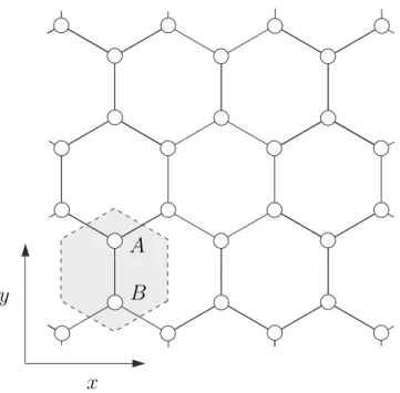
A
B
x
y
Figure 1.5. The two dimensional honeycomb lattice of graphene. The hexagonal unit cell is indicated by a shaded hexagon. Each unit cell contains two atoms, one belonging to theAsublattice and one to theB sublattice.
answered in 2004 when the group of Andrei Geim in Manchester reported the successful fabrication of graphene devices for electron transport experi-ments [33]. Subsequent experimental studies, particularly those performed in the quantum Hall regime [34, 35], confirmed the theoretical prediction that low energy excitations are described by a two dimensional Dirac equa-tion. Several tutorials [36, 37, 38, 39, 40] and reviews [41, 42, 43, 44] pro-vide an overview of recent developments. Here we discuss only the very basics.
Graphene has a two dimensional honeycomb lattice. A honeycomb lattice consists of two triangular sublattices denotedA and B. These are arranged such that each A (B) sublattice site is at the centroid of the
triangle formed by its nearest neighbor sites. These neighboring sites all belong to theB(A) sublattice. This is illustrated in Fig. 1.5. The distance between nearest neighbors on the lattice isa≃1.42Å.
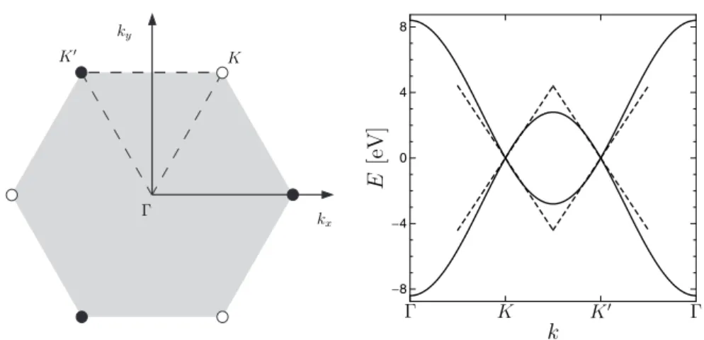
de-K K′
Γ k
x ky
-8 -4
0 4 8
Γ K K′
Γ
k
E
[e
V
]
Figure 1.6. Left panel: The Brillouin zone of the graphene lattice. The K
and K′ points at the corners of the Brillouin zone are indicated by open and
filled circles respectively. The threeK points are connected by reciprocal lattice vectors and are therefore equivalent. The same holds for the K′ points. There
is no reciprocal lattice vector connecting K and K′, and these two corners are
inequivalent. The center of the Brillouin zone is at the pointΓ. The dashed lines indicate the contour along which the dispersion is plotted in the right panel. Right panel: The energy dispersion of graphene along the lines ΓK, K K′, and K′Γ
in the Brillouin zone. At the two inequivalent cornersKandK′, the conduction
and valence bands touch at energyE= 0, the Fermi energy of undoped graphene. These are called Dirac points. Close to the Dirac points the dispersion of both the conduction and valence bands are linear. The associated excitations (particles or holes) are described by the Dirac equation (1.25).
picted in Fig. 1.6. Below we will see that wave vectors in the corners of the Brillouin zone are relevant for describing low-energy excitation. We therefore mention that the six corners of the Brillouin zone can be par-titioned into two sets of three, indicated in Fig. 1.6 by black and white dots respectively. Members of the same set are connected by basis vectors of the reciprocal lattice and hence refer to the same physical state. This means that the Brillouin zone has two inequivalent corners. We take these to be
K = 2π 3a
ˆ
x+√1
3yˆ
, K′ = 2π 3a
−xˆ+√1
3yˆ
. (1.24)
binding Hamiltonian. To good approximation only nearest neighbor hop-ping has to be taken into account. The nearest neighbor hophop-ping energy is t ≃ 3 eV. The resulting energy dispersion is shown in Fig. 1.6. It is
seen that the conduction and valence bands touch. Touching occurs at so-called Dirac points situated at the corners of the Brillouin zone. The energy at which the bands touch is equal to the Fermi energy of undoped graphene. Like a semi-conductor, undoped graphene therefore has a filled valence band and an empty conduction band. Unlike a semi-conductor though, there is no energy gap between the valence and conduction bands. Graphene is therefore called a semi-metal.
We now examine the dispersion relation close to one of the two in-equivalent Dirac points. To be definite, let us consider the Dirac point at
K. We definep=~(k−K) as the momentum associated with the wave
vectork and measured from a reference point~K. In the vicinity of ~K,
the dispersion relation readsE=±v|p|where v= 3ta/2≃106m/s is the
Fermi velocity. This describes two cones touching at the Dirac point. The positive sign refers to the conduction band while the negative sign refers to the valence band. Excitations travel at a group velocityvg =∇pE =±vpˆ.
The magnitude of the group velocity is equal to the Fermi velocity, inde-pendent of energy. Electrons in graphene behave like massless relativistic particles, traveling at the effective speed of light v regardless of their
en-ergy.
For excitations close to the Fermi energy of undoped graphene, the tight binding Hamiltonian can be expanded in momentum around either of the Dirac points. We consider here states in the vicinity of theK point.
A continuum description results in which the electron wave functionΨ(r)
is defined on the wholex-y plane such thatexp(iK·r)×Ψ(r)interpolates
the value of the tight-binding wave function defined on the honeycomb lattice. The continuum wave function Ψ satisfies EΨ = HΨ where H is the Dirac Hamiltonian
H=v(p−α)·σ+φ. (1.25) Here α is e times the magnetic vector potential in the x-y plane and φ
is e times the electric scalar potential. Both of these have to be smooth
on the scale of the inter-atomic distancea. In position representation, the
momentum isp=−i~(∂x, ∂y). The vectorσ = (σx, σy)contains the Pauli
matrices
σx=
0 1 1 0
, σy =
0 −i i 0
The Hamiltonian acts on spinorsΨ = (ψA, ψB), withψAthe amplitude to be on the A sublattice and ψB the amplitude to be on the B sublattice. This spinor degree of freedom is called pseudospin to distinguish it from the real electron spin, which does not appear in the Eq. (1.25).
The excitations around the Dirac point atK′ are also described by the
Dirac Hamiltonian of Eq. (1.25). The fact that excitations around both Dirac points are present in weakly doped graphene results in a two-fold degeneracy of eigenstates. The associated degree of freedom is called the valley index. As long as the spatial variation of α andφis smooth on the
scale of the inter-atomic distance a, and we restrict ourselves to energies
E ≪ ~v/a, the valleys remain uncoupled in an infinite graphene sheet.
At the edges of a finite sheet however, the valleys can be coupled by the boundary [45].
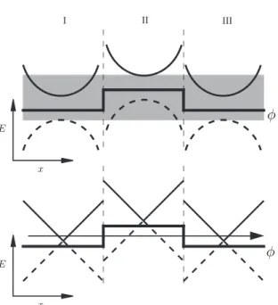
The Dirac equation gives rise to unusual transport properties. This is illustrated by the following example. Consider an electrostatic potential barrier φ(r) in the region 0< x < L. Usually such a potential introduces
scattering. A particle incident on φfrom the left (x <0) is reflected back with probability R and transmitted to the right (x > L) with probability T = 1−R. If the energyE of the incident particle is less than the barrier
height, transmission through the barrier is strongly suppressed and the reflection probability tends to unity. For energies larger than the barrier height, the probability for transmission becomes finite. However, only in the limit E ≫maxφdoes the transmission probability approach unity.
I II III
x x
E E
φ φ
Furthermore, at normal incidence, transmission is always perfect. To see this, we solve the Dirac equation with φ(x) that depends only on the x-coordinate. We focus on incident waves that propagate normal to the
potential barrier. (Normal incidence means that the wave number in they -direction is zero, and the wave function only depends on thexcoordinate.)
In this case, the time-independent Dirac equation for given energy E can
be rewritten as
∂xΨ(x) =
i
~vσx[E−φ(x)] Ψ(x), (1.27)
and the solution is found by straight-forward integration. Correspond-ing to any energy E, we find a left-incident (+) and a right-incident (−) solution
Ψ±(x) =
e±iEx/~v √
2
1
±1
×
1 x <0
exp ∓iR0xdx′φ(x′)/~v 0< x < L exp∓iR0Ldx′φ(x′)/~v x > L
.
(1.28) Remarkably, these wave functions each contain an incident component and a transmitted component but no reflected component. At normal incidence, the transmission probability is always unity. This is particularly striking for incident energies smaller than the height of the potential barrier where one would normally expect almost perfect reflection.
The phenomenon we have just encountered is sometimes referred to as the absence of back-scattering in graphene [48]. It has some surprising consequences. Adding disorder to a graphene sample can enhance the conductivity [49, 50]. Furthermore, disorder that is smooth on the scale of the lattice constant cannot turn graphene into an insulator [51, 52, 53].
1.5
Bilayer graphene
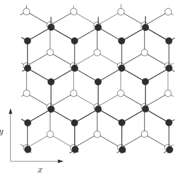
In Chapter 5 of this thesis we consider bilayer graphene, i.e. two layers of carbon atoms one on top of the other. The way the two layers are stacked is illustrated in Fig. 1.8. TheAsublattice of the one layer is directly above
theB sublattice of the other. Bilayer graphene has a unit cell containing
x
y
Figure 1.8. A graphene bilayer consists of two monolayers stacked one on top of the other. In order to be able to distinguish the two layers, open circles were used to indicate carbon atoms in the bottom layer while filled circles were used to indicate carbon atoms in the top layer. The B sublattice of the top layer is directly above theAsublattice of the bottom layer.
the bilayer is described by a4×4long wavelength Hamiltonian [54, 55, 56]
H =
φ v(px−ipy) t⊥ 0
v(px+ipy) φ 0 v3(px−ipy)
t⊥ 0 φ v(px+ipy) 0 v3(px+ipy) v(px−ipy) φ
. (1.29)
(We only consider the case of zero magnetic field.) The upper left 2×2
block is the Dirac Hamiltonian of Eq. (1.25) and describes the electron dynamics inside one layer. The lower right 2×2 block is obtained by interchanging the A and B sublattices in the Dirac Hamiltonian and
v3 breaks the isotropy of the dispersion relation, introducing a triangular
distortion known as “trigonal warping”. In Chapter 5 we ignore this com-plication and calculate the transport properties of the bilayer for v3 = 0.
A complete calculation, including the effects of trigonal warping, has sub-sequently been published in Refs. [57, 58].
1.6
This Thesis
1.6.1 Chapter 2
In Chapter 2 we present a derivation of the Keldysh action of a general multi-channel time-dependent scatterer in the context of the Landauer-Büttiker approach. This result is then applied in two subsequent chapters. In general the Keldysh action of a system is defined asA= lnZ, where
Z= Tr
T+exp
−i Z t1
t0
dtH+(t)
ρ0T−exp
i
Z t1 t0
dtH−(t)
.
(1.30) In this expression, ρ0 is the initial density matrix of the system. This is
evolved forwards and backwards in time with two different time-dependent Hamiltonians H±(t). For the purpose of this introduction we set H± =
H+χ±(t)Qwhere H is the actual Hamiltonian of the system,Qis a sys-tem coordinate andχ±(t) are arbitrary functions of time. (Generalization to more fields, each coupling to a different system coordinate, is straight forward.) Z and A are functionals of χ±. The ordering symbol T+
in-dicates time-ordering of operators with the largest time-argument to the left, while T− time-orders with the largest argument to the right.
Why are we interested in this object? Let us firstly mention its most direct application, namely to evaluate time-ordered correlators of the co-ordinate Q. This is done by taking functional derivatives with respect to χ+(t) and χ−(t). We obtain
* T− M Y j=1
Q(tj)
T+
N
Y
k=1
Q(t′k)
!+ = M Y j=1
−i δ
δχ−(t j) N Y k=1 i δ
δχ+(t′ k)
Z[χ]
A less obvious application is the following. Suppose the coordinateQof the system for which we knowA(call it system A) is coupled to another system (B). Knowing A[χ±], we can then calculate the influence that system A has on system B. (For this reason Feynman and Vernon [8] call Z the influence functional.) In chapters 3 and 4 for instance, we calculate how specific measuring devices respond when coupled to a coherent conductor, starting from an expression for the Keldysh actionA of the conductor.
Previous studies of the Keldysh action focused on weakly interacting disordered electron systems [59, 60]. We consider the Keldysh action of an arbitrary coherent conductor connected to electron reservoirs. For such systems an explicit expression forA[χ]was known (see for instance
Chap-ter 3 or Ref. [61]) only in the case where the fieldsχ±couple to electrons in the reservoirs rather than in the scattering region. We wanted to consider a setup where the scattering potential depends on the state of an adjacent quantum system (Chapter 4). In Chapter 2 we therefore generalized the known result for the actionAto the situation where the fields χ± couple to electrons inside the scattering region.
1.6.2 Chapter 3
In Chapter 3 we analyze the operation of a quantum tunneling detector coupled to a coherent conductor. Use is made of the theory developed in Chapter 2. The coherent conductor is biased with a voltage V. The circuit that connects the coherent conductor to the voltage biased elec-tron reservoirs has a finite impedance. As a result, current fluctuations in the coherent conductor are converted into voltage fluctuations on top of V. The fluctuations are detected as photons. The detector is
capa-ble of frequency-resolved detection. We demonstrate that for frequencies larger than eV /2π~, the output of the detector is determined by
1.6.3 Chapter 4
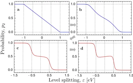
In Chapter 4 we study a charge qubit with level splitting ε coupled to a quantum point contact (QPC) driven by a bias voltage V. The charge
qubit can be realized by the lowest two eigenstates of an electron trapped in double quantum dot. The qubit Hilbert space is spanned by a state |1irepresenting the electron localized in one dot, together with a state|2i representing the electron localized in the other dot. Because of the coupling to the qubit, the scattering matrix of the QPC depends on the state of the qubit. We define the qubit polarization as the probability to find the qubit in state |1i. For given V, we calculate the the qubit polarization as
a function of the qubit level splitting. Use is made of the theory developed in Chapter 2. In the limit of weak coupling, the qubit polarization shows cusps at ε=±eV. We show that, for stronger couplings, a plateau occurs
for |ε| ≤ ±eV /2. Further increase of the coupling leads to a polarization
p2= [1 + exp(βε)]−1 corresponding to an effective temperatureβ−1 ∼eV.
1.6.4 Chapter 5
Here we calculate the Fermi energy dependence of the (time-averaged) current and shot noise in an impurity-free carbon bilayer (length L ≪ width W), and compare with known results for a monolayer [62]. We
model the interlayer coupling by means of a hopping element t⊥ =~v/l⊥ between nearest neighbors in different layers. Here l⊥ is the inter-layer hopping length estimated to be on the order of ten times the inter-atomic distance. At the Dirac point of charge neutrality, the bilayer (l⊥ finite) transmits as two independent monolayers in parallel (l⊥ infinite): Both current and noise are resonant at twice the monolayer value, so that their ratio (the Fano factor) has the same 1/3 value as in a monolayer — and the same value as in a diffusive metal. The range of Fermi energies around the Dirac point within which this pseudo-diffusive result holds is smaller, however, in a bilayer than in a monolayer (by a factor l⊥/L). It was subsequently shown by Moghaddam and Zareyan [58] that this conclusion holds only for lengths less than about 50 nm (≃30times l⊥), because we ignored the effects of trigonal warping mentioned in Sec. 1.5.
1.6.5 Chapter 6
creates two regions, onep-doped and onen-doped. In thep-doped region,
the Fermi energy is in the conduction band while in then-doped region it
is in the valence band. We consider the regime where the Hall conductance in both thep-doped andn-doped regions is 2e2/h. We calculate the
two-terminal conductanceG. In the absence of intervalley scattering, the result G = (e2/h)(1−cos Φ) depends only on the angle Φ between the valley
isospins (= Bloch vectors representing the spinor of the valley polarization) at the two opposite edges. This plateau in the conductance versus Fermi energy is insensitive to electrostatic disorder, while it is destabilized by the dispersionless edge state which may exist at a zigzag boundary. A strain-induced vector potential shifts the conductance plateau up or down by rotating the valley isospin.
1.6.6 Chapter 7
Appendix 1.A
The Keldysh technique: an
example
In this appendix we illustrate the use of the Keldysh technique with the following example. A quantum dot is connected to two reservoirs by means of tunnel barriers. One reservoir is grounded and we measure all energies relative to its Fermi energy. For times t < 0 the other reservoir is held
at zero voltage too, and the dot is neutral and in equilibrium with the reservoirs. Consequently, the dot’s chemical potentialµ(t)is zero fort <0. For times t >0, a time-dependent voltageV(t)is applied to one reservoir.
We want to calculate the expectation value of the charge on the dot, as a function of time.
The dot can be modeled as a set of independent levels that are con-nected to reservoirs by tunneling. They are labeled by an integer m. The
Green function Gis diagonal in this basis, i.e. Gm,n(t, t′) =δm,nGm(t, t′). Note that, since am(t) and a†m(t) anti-commute to unity at coinciding times, the Keldysh Green function contains information about the occu-pation probability of levels. More precisely
Km(t, t) =−i[1−2nm(t)], nm(t) =
D
a†m(t)am(t)
E
, (1.32)
with nm(t) the probability that level m is occupied at time t. The to-tal number of electrons n(t) on the dot is the sum of all the occupation
probabilities n(t) =Pmnm(t).
The Green functionGm(t, t′) obeys the following equations
i∂tGm(t, t′)−[εm+µ(t)]Gm(t, t′)
−
Z
d˜tΣ(t,˜t)Gm(˜t, t′) =δ(t−t′)I2×2, (1.33a)
−i∂t′Gm(t, t′)−εm+µ(t′)Gm(t, t′) −
Z
d˜t G′m(t,˜t)Σ(˜t, t′) =δ(t−t′)I2×2. (1.33b)
A chemical potentialµ(t)takes into account charging effects: When charge
on the dot fluctuates so that it is no longer neutral, work has to be done against the electric field of the excess charge Q(t) in order to add more
charge to the dot. µ(t)is proportional toQ(t), the proportionality constant
being the capacitance C of the dot:
µ(t) = 1
Assuming that the dot is neutral at timet= 0, Q(t) = n(t)−n(0). The self-energy describes the tunneling of electrons between the dot and the reservoirs. Its components are explicitly
Σ(R)(t, t′) = −iEThδ(t−t′), (1.35a)
Σ(A)(t, t′) = iEThδ(t′−t), (1.35b)
Σ(K)(t, t′) = −2ETh π
1 t−t′
n
αe−i[ψ(t)−ψ(t′)]+ 1−αo. (1.35c) In this equationETh is the Thouless energy, or inverse lifetime of an
elec-tron on the dot. It characterizes the time an elecelec-tron spends on the dot before tunneling through one of the tunnel barriers. The phase ψ(t) is
the integral of the reservoir voltage ψ(t) =R0tdt′V(t′) and α ∈[0,1]is a
parameter that measures the relative coupling to the reservoirs. The value
α = 0.5 corresponds to equally strong couplings to both reservoirs while
α= 0corresponds to the dot completely decoupled from the voltage-biased
reservoir and α = 1 corresponds to the dot entirely decoupled from the
grounded reservoir.
We now solve Eq. (1.33), starting with the retarded component, i.e. the upper-left block, which reads explicitly
i∂tRm(t, t′)−[εm+µ(t)−iETh]Rm(t, t′) =δ(t−t′), (1.36a) −i∂t′Rm(t, t′)−[εm+µ(t)−iETh]Rm(t, t′) =δ(t−t′). (1.36b)
The retarded Green functionRm(t, t′)is defined as an anti-commutator of a creation and an annihilation operator. Since the creation and annihilation operators anti-commute at coinciding times, it follows that
lim
t−t′→0+Rm(t, t
′) =−i. (1.37)
Furthermore, by definition, Rm(t, t′ > t) = 0. Imposing these conditions leads to the unique solution
Rm(t, t′) =−iθ(t−t′)e−ETh(t−t ′)
e−iεm(t−t′)e−i[φ(t)−φ(t′)], (1.38)
where φ(t) is the integral of the chemical potential µ; φ(t) =R0tdt′µ(t′).
We see that Rm(t, t′) decays exponentially as a function of t−t′ with lifetime ETh−1. To understand why this is, note that the two terms that constitute the retarded Green function have the following interpretation. Term Dam(t)a†m(t′)
E
at time t′ will still be there at time t. The term a†m(t′)am(t) is (the complex conjugate of) the amplitude that, if an electron is removed from level m at time t′, that level will still be empty at time t. When the dot is coupled to reservoirs, these can populate and depopulate the levels, causing the amplitudes represented by Rm(t, t′) to decay. Similarly, one finds that the advanced Green function is given by
Am(t, t′) =iθ(t′−t)e−ETh(t ′−t)
e−iεm(t−t′)e−i[φ(t)−φ(t′)]. (1.39)
It remains for us to consider the Keldysh component of Eq. (1.33). We start by taking a brief look at the Keldysh component of the self-energy. It should be thought of as consisting of two contributions.
Σ(K)(t, t′)i = 2iEThα σV(t, t′) + (1−α)σ0(t, t′), (1.40a)
σV(t, t′) =
i π
e−i[ψ(t)−ψ(t′)]
t−t′ . (1.40b)
The σ0 contribution accounts for the coupling to the grounded reservoir.
Note that it can be written as
σ0(t, t′) =
Z dε
2πe
−iε(t−t′)
[1−2f(ε)], (1.41)
where f0(ε) = θ(−ε) is the zero-temperature Fermi distribution of
elec-trons in the grounded reservoir. The σV contribution similarly accounts for the presence of the reservoir with fluctuating bias voltage. Suppose for instance that the bias voltage V is constant. Thenψ(t) =V t andσV can be written as
σV(t, t′) =
Z dε 2πe
−iε(t−t′)
[1−2f(ε−V)]. (1.42)
Again the zero-temperature Fermi distribution appears, this time with the Fermi energy appropriately shifted byV relative to the grounded reservoir.
The fact that the reservoir distribution functions only appear in the Keldysh component of the self-energy illustrates the following general prin-ciple. The retarded and advanced functions determine the effective one-body spectrum, while Keldysh functions determine how states are popu-lated.
We now solve for the Keldysh component of the dot Green function. The upper right block of Eq. (1.33a) reads
[i∂t−εm−µ(t) +iETh]Km(t, t′) =
Z
We invoke Eq. (1.36) which says thatRm(t, t′)is a resolvent for the differ-ential operator appearing on the left of the above equation. Additionally we impose the initial condition that the system was in equilibrium before the time-dependent voltage was switched on. This implies the solution
Km(t, t′) =
Z
dt1dt2Rm(t, t1)Σ(K)(t1, t2)Am(t2, t′). (1.44)
So, we have found Km(t, t′). Are we done yet? Not quite. We still have to determine the chemical potentialµ(t). In order to do this, we have
Eq. (1.34) that relatesµ(t) to the excess charge Q(t)on the dot, which in
turn is related to the Keldysh Green function at coinciding times. Putting these together, we have
Q(t) =−i 2
X
m
Km(t, t)−Km(0,0). (1.45)
We use the solution (Eq. 1.44) forKm, with the explicit form of Rm and
Am substituted from Eqs. (1.38) and (1.39) to obtain
Q(t) =−i 2
X
m
Z 0
−∞
dt1dt2eETh(t1+t2)e−iεm(t2−t1)
×ne[φ(t+t1)−φ(t+t2)]Σ(K)(t+t
1, t+t2)−Σ(K)(t1, t2)
o
| {z }
X
, (1.46)
where we have explicitly used the fact that µ(t) and hence φ(t) are zero
fort <0.
Let us assume that the mean level spacingδεis much smaller than the
Thouless energy. Then we can replace
X
m
e−iεm(t2−t1)→δ(t
2−t1)
2π
δε. (1.47)
This is substituted into Eq. (1.46). The delta-function picks out thet2→
t1limit of the expression markedX. The factor1/(t1−t2)inΣ(K)results
in time-derivatives ofψ andφ, so that
lim t2→t1
X=−2iETh
Using µ(t) =Q(t)/C, we obtain an integral equation for µ(t)namely
µ(t) =−2ETh Cδε
Z t −∞
dt′e−2ETh(t−t′)µ(t′)−αV(t′). (1.49)
This is converted into a differential equation by multiplying with e2ETht and taking a time-derivative. Finally we obtain
d
dtµ(t) +γ µ(t) = ΓV(t), (1.50)
with Γ = 2αETh/Cδε and γ = 2ETh(1 + 1/Cδε). We solve this, and
multiply by the capacitance, to obtain the charge on the dot as a function of time
Q(t) = 2αETh δε
Z t
0
dt′e−γ(t−t′)V(t′). (1.51)
It is instructive to compare this result to conclusions drawn from the following intuitive argument. We suppose that the quantum system we just analyzed is roughly equivalent to the an electric circuit where a cen-tral region with capacitance C is connected to leads 1 and 2, by means of resistors R1 and R2 respectively. Lead 2 is grounded while a
time-dependent voltage V(t) is applied to lead 1. The voltage of the central
region is µ(t). It is related to the excess charge Q(t)on the central region by µ(t) = Q(t)/C. If I1 is the current flowing from the lead 1 into the
central region and I2 is the current flowing from the central region into
lead 2then, Ohm’s law says
I1(t) = [V(t)−µ(t)]/R1, I2(t) =µ(t)/R2. (1.52)
Charge conservation implies that dQ(t)/dt=I1(t)−I2(t). Putting
every-thing together, we obtain a differential equation for µ(t):
d
dtµ(t) +γclµ(t) = ΓclV(t), (1.53)
where γcl= (R−11+R2−1)/C andΓcl= 1/R1C.
This has the same form as the differential equation (1.50) that we ob-tained previously. However, if we compare the relaxation ratesγandγclwe
note an important difference. In the limitδεC ≫1, the classical relaxation
rateγcl goes to zero, whileγ obtained with the Keldysh technique remains
relaxes into the reservoirs. The limit of large capacitance C corresponds to a situation where the Coulomb repulsion between electrons on the dot is weak. Even in this limit, excess charge on the dot should relax into the leads. The reason is that, due to the dynamics of non-interacting electrons on the dot, every once in a while, an electron tunnels into a reservoir. This process does not require that the escaping electron be “pushed off the dot” by the other electrons. The classical argument ignores the dynamics of non-interacting electrons, so that the only method for charge to leak off the dot is through Coulomb repulsion. Hence the classical and quantum results can only be expected to agree in theδε≪C−1 limit. Beyond this
limit, the quantum mechanical analysis, based on the Keldysh technique remains valid, while the classical argument breaks down.
We can relate the resistancesR1 and R2 of the classical theory to the
parameters of the quantum theory in theδε≪C−1 limit. One obtains
R−11= 2αETh δε
e2
~, R
−1
2 = 2(1−α)
ETh
δε e2
~, (1.54)
where e2/~ reinstates the units that where dropped in the microscopic
analysis. The quantity ETh/δε is known to characterize the conductance
[1] R. Landauer, IBM J. Res. Dev. 1, 223 (1957); Philos. Mag. 21, 863 (1970).
[2] M. Büttiker, IBM J. Res. Dev. 32, 63 (1988).
[3] C. W. J. Beenakker and H. van Houten, Solid State Phys.44, 1 (1991).
[4] H. van Houten, C. W. J. Beenakker, J. G. Williamson, M. E. I. Broekaart, P. H. M. van Loosdrecht, B. J. van Wees, J. E. Mooij, C. T. Foxon and J. J. Harris, Phys. Rev. B 39, 8556 (1989).
[5] Ya. M. Blanter and M. Büttiker, Phys. Rep. 336, 1 (2000).
[6] C. W. J. Beenakker and C. Schönenberger, Phys. Today 56 (5), 37 (2003).
[7] L. V. Keldysh, Zh. Eksp. Teor. Fiz.47, 1515 (1964); [Sov. Phys. JETP 20, 1018 (1965)].
[8] R. P. Feynman and F. L. Vernon Jr., Ann. Phys. (N. Y.) 24, 118 (1963).
[9] J. Schwinger, J. Math. Phys. 2, 407 (1961).
[10] J. Rammer and H. Smith, Rev. Mod. Phys. 58, 323 (1986).
[11] E. M. Lifshitz and L. P. Pitaevskii, Physical Kinetics, (Pergamon
Press, Oxford, 1981).
[12] A. Kamenev, arXiv:cond-mat/0412296.
[14] A. A. Abrikosov, L. P. Gorkov and I. E. Dzyaloshinski, Methods of Quantum Field Theory in Statistical Physics, (Prentice-Hall, New
Jer-sey, 1963).
[15] J. W. Negele and H. Orland, Quantum Many-Particle Systems,
(Addison-Wesley, California, 1987).
[16] M. Kindermann, Yu. V. Nazarov and C. W. J. Beenakker, Phys. Rev. Lett. 90, 2468051 (2003).
[17] M. Kindermann, Yu. V. Nazarov and C. W. J. Beenakker, Phys. Rev. B69, 035336 (2004).
[18] G.-L. Ingold and Yu. V. Nazarov, inSingle Charge Tunneling, edited
by H. Grabert and M. H. Devoret, NATO ASI Series B294 (Plenum, New York, 1992).
[19] G. Schön, Phys. Rev. B32, 4469 (1986).
[20] M. H. Devoret, D. Esteve, H. Grabert, G.-L. Ingold, H. Pothier and C. Urbina, Phys. Rev. Lett.64, 1824 (1990).
[21] S. M. Girvin, L. I. Glazman, M. Jonson, D. R. Penn and M. D. Stiles, Phys. Rev. Lett.64, 3183 (1990).
[22] A. Levy Yeyati, A. Martin-Rodero, D. Esteve and C. Urbina, Phys. Rev. Lett. 87, 046802 (2001).
[23] A. O. Caldeira and A. J. Leggett, Phys. Rev. Lett.46, 211 (1981).
[24] A. O. Caldeira and A. J. Leggett, Ann. Phys. (N. Y.)149, 374 (1983).
[25] Yu. V. Nazarov and D. V. Averin, Physica B162, 309 (1990).
[26] Yu. V. Nazarov, Phys. Rev. B 43, 6220 (1991).
[27] J. J. Sakurai, Advanced Quantum Mechanics, (Addison-Wesley,
Massechusetts, 1967).
[28] P. R. Wallace, Phys. Rev.71, 622 (1947).
[29] J. W. McClure, Phys. Rev.104, 666 (1956).
[31] D. P. DiVincenzo and E. J. Mele, Phys. Rev. B 29, 1685 (1984).
[32] F. D. M. Haldane, Phys. Rev. Lett. 61, 2015 (1988).
[33] K. S. Novoselov, A. K. Geim, S. V. Morozov, D. Jiang, Y. Zhang, S. V. Dubonos, I. V. Grigorieva and A. A. Firsov, Science 306, 666 (2004).
[34] K. S. Novoselov, A. K. Geim, S. V. Morozov, D. Jiang, M. I. Katsnel-son, I. V. Grigorieva, S. V. Dubonos and A. A. Firsov, Nature 438, 197 (2005).
[35] Y. Zhang, Y.-W. Tan, H. L. Stormer and P. Kim, Nature 438, 201 (2005).
[36] A. H. Castro Neto, F. Guinea and N. M. R. Peres, Phys. World 19, 33 (2006).
[37] A. K. Geim and K. S. Novoselov, Nature Mat. 6, 183 (2007).
[38] A. K. Geim and A. H. MacDonald, Phys. Today 60(8), 35 (2007).
[39] M. I. Katsnelson, Materials Today 10, 20 (2007).
[40] A. K. Geim and P. Kim, Scientific American 298(4), 90 (2008).
[41] A. H. Castro Neto, F. Guinea, N. M. R. Peres, K. S. Novoselov and A. K. Geim, arXiv:0709.1163 (2007).
[42] V. P. Gusynin, S. G. Sharapov and J. P. Carbotte, Int. J. Mod. Phys. B21, 4611 (2007).
[43] M. I. Katsnelson and K. S. Novoselov, Solid State Comm. 143, 3 (2007).
[44] C. W. J. Beenakker, arXiv:0710.3848 (2007).
[45] L. Brey and H. A. Fertig, Phys. Rev. B 73, 195408 (2006).
[46] V. V. Cheianov and V. I. Fal’ko, Phys. Rev. B 74, 041403(R) (2006).
[48] T. Ando, T. Nakanishi and R. Saito, J. Phys. Soc. Japan 67, 2857 (1998).
[49] M. Titov, Europhys. Lett.79, 17004 (2007).
[50] A. Rycerz, J. Tworzydło and C. W. J. Beenakker, Europhys. Lett. 79, 57003 (2007).
[51] J. H. Bardarson, J. Tworzydło, P. W. Brouwer and C. W. J. Beenakker, Phys. Rev. Lett. 99, 106801 (2007).
[52] K. Nomura, M. Koshino and S. Ryu, Phys. Rev. Lett. 99, 146806 (2007).
[53] P. San-Jose, E. Prada and D. S. Golubev, Phys. Rev. B 76, 195445 (2007).
[54] E. McCann and V. Fal’ko, Phys. Rev. Lett.96, 086805 (2006).
[55] J. Nilsson, A. H. Castro Neto, F. Guinea and N. M. R. Peres, Phys. Rev. Lett. 97, 266801 (2006).
[56] J. Nilsson, A. H. Castro Neto, F. Guinea and N. M. R. Peres, Phys. Rev. B 93, 214418 (2006).
[57] J. Cserti, A. Csordás and G. Dávid, Phys. Rev. Lett. 99, 066802 (2007)
[58] A. G. Moghaddam and M. Zareyan, arXiv:0804.2748 (2008).
[59] A. Kamenev and A. Andreev, Phys. Rev. B60, 2218 (1999).
[60] M. V. Feigel’man, A. I. Larkin and M. A. Skvortsov, Phys. Rev. B 61, 12361 (2000).
[61] M. Kindermann and Yu. V. Nazarov, Phys. Rev. Lett. 91, 136802 (2003).
[62] J. Tworzydło, B. Trauzettel, M. Titov, A. Rycerz and C. W. J. Beenakker, Phys. Rev. Lett. 96, 246802 (2006).
[63] J. T. Chalker and P. D. Coddington, J. Phys. C21, 2665 (1988).
The Keldysh action of a
time-dependent scatterer
2.1
Introduction
The pioneering works of Landauer [1] and Büttiker [2] lay the foundations for what is now known as the scattering approach to electron transport. The basic tenet is that a coherent conductor is characterized by its scat-tering matrix. More precisely the transmission matrix defines a set of transparencies for the various channels or modes in which the electrons propagate through the conductor. As a consequence, conductance is the sum over transmission probabilities. Subsequently, it was discovered that the same transmission probabilities fully determine the current noise, also outside equilibrium, where the fluctuation-dissipation theorem does not hold [3].
superconductors [16].
Many of these more advanced applications are unified through a method developed by Feynman and Vernon for characterizing the effect of one quantum system on another when they are coupled [17]. The work of Feynman and Vernon dealt with the effect of a bath of oscillators cou-pled to a quantum system. It introduced the concept of a time-contour describing propagation first forwards then backwards in time. By using the path-integral formalism, it was possible to characterize the bath by an “influence functional” that did not depend on the system that the bath was coupled to. This functional was treated non-perturbatively. A related development was due to Keldysh [18]. While being a perturbative dia-grammatic technique, it allowed for the treatment of general systems and shared the idea of a forward and backward time-contour with Feynman and Vernon.
In general, the Feynman-Vernon method expresses the dynamics of a complex system in the form of an integral over a few fieldsχ(t). Each part
of the system contributes to the integrand by a corresponding influence functionalZ[χ], or, synonymously, a Keldysh actionA[χ] = lnZ[χ]. Thus the Keldysh action of a general scatterer can be used as a building block. In this way the action of a complicated nanostructure consisting of a network of scatterers can be constructed. As in the case of classical electronics, a simple set of rules, applied at the nodes of the network, suffice to describe the behavior of the whole network [19, 20].
The essential element of the approach is that the fieldsχtake different
values on the forward/backward parts of the time-contour. One writes this asχ±(t), where+ (−) corresponds to the forward (backward) part of the contour. The Keldysh action for a given sub-system is evaluated as the full non-linear response of the sub-system to the fieldsχ±(t). (See Eq. 2.6 below for the precise mathematical definition.)
Applications involving the scattering approach require both the notion of the non-perturbative influence functional and the generality of Keldysh’s formalism. Until now, the combination of the Feynman-Vernon method with the scattering approach was done on a case-specific basis: Only those elements relevant to the particular application under consideration were developed. In this paper we unify previous developments by deriving gen-eral formulas for the Keldysh action of a gengen-eral scatterer connected to charge reservoirs.
Hamiltoni-ansH+(t)andH−(t)that governs forward and backward evolution in time
respectively. Since we are in the framework of the scattering approach, these field-dependent Hamiltonians are not the most natural objects to work with. Rather, depending on where the fields couple to the system, it is natural to incorporate their effect either in the scattering matrix of the conductor, or in the Green functions of the electrons in the reservoirs: The fields affecting the scattering potential inside the scatterer are incorporated in a time-dependent scattering matrix. Since the fieldsχ±for forward and backward evolution are different, the scattering matrices for forward and backward evolution differ. The effect of the fields perturbing the electrons far form the scatterer is incorporated in the time-dependent Green func-tions of the electrons in distant reservoirs. A bias voltage applied across a conductor can conveniently be ascribed to either Green functions of the reservoirs or to a phase factor of the scattering matrix. The same holds for the counting fields encounterd in the theory of full counting statistics. There are however situations where our hand is forced. For instance, in the example of the Fermi-edge singularity, that we discuss in Sec. 2.6, the time-dependent fields have to be incorporated in the scattering matrices.
Previous studies of the Keldysh action concentrated on situations where the fieldsχ±could be incorporated in the reservoir Green functions. These studies therefore assumed stationary, contour-independent scatter-ing matrices while allowscatter-ing for a time-dependence and/or time-contour dependence of the electron Green functions. Early works (Refs. [21] and [22]) used an action of this type to analize Coulomb blockade phenomena. Later, the same action was understood in the wider context of arbitrary Green’s functions [19, 23]. In this form it has been used to treat problems involving for example interactions and superconductivity. The action em-ployed in these studies corresponds to Eq. 2.4 and can readily be derived in the context of non-linear sigma-model of disordered metals [24].
The main innovation of the present work is to generalize the action to contour- and time-dependent scattering matrices. The only assumption we make is that scattering is instantaneous: We do not treat the delay time an electron spends inside the scattering region realistically.
the real line. The forward (backward) scattering matrixsˆ+ (−)with kernel
s(α= + (−);c, c′;t) obeys the usual unitarity condition ˆs†±sˆ±= 1.
With the aide of these preliminary definitions, our main result is sum-marized by a formula for the Keldysh action.
A[ˆs] = Tr ln
"
1 + ˆG 2 + ˆs
1−Gˆ 2
#
−Tr ln ˆs−. (2.1)
In this formula,Gˆ is the Keldysh Green function characterizing the
reser-voirs connected to the scatterer [25]. It is to be viewed as an operator with kernel G(α, α′;c;t, t′)δc,c′ where indices carry the same meaning as in the definition ofsˆ. This formula is completely general.
1. It holds for time dependent scattering matrices that differ on the forward and backward time contour.
2. It holds for multi-terminal devices with more than two reservoirs.
3. It holds for devices such as Hall bars where particles in a single chiral channel enter and leave the conductor at different reservoirs.
4. It holds when reservoirs cannot be characterized by stationary filling factors. Reservoirs may be superconducting, or contain “counting fields” coupling them to a dynamical electromagnetic environment or a measuring device.
When the reservoirs can indeed be characterized by filling factorsfˆ(ε),
the Keldysh structure can explicitly be traced out to yield
A[ˆs+,sˆ−] = Tr ln
h
ˆ
s−(1−fˆ) + ˆs+fˆ
i
−Tr ln ˆs−. (2.2)
In this expression operators retain channel structure and time structure. In “time” representation,fˆis the Fourier transform to time of the reservoir
filling factors, and as such has a kernel f(c;t, t′)δc,c′ diagonal in channel space and depending on two times. In stationary limit, this formula im-mediately reduces to the Levitov formula for low-frequency Full Counting Statistics (FCS) [5].
terminal may still be connected to the scatterer by an arbitrary number of channels. We denote the two terminals left (L) and right (R). In this case the reservoir Green function has the form
ˆ G=
ˇ GL 0
0 GˇR
channel space
, (2.3)
where Gˇ
L(R) have no further channel space structure. Matrix structure in
Keldysh and time indices (indicated by a check sign) is now retained in the trace, but the channel structure is traced out. Thus is obtained
A[χ±] =
1 2
X
n Tr ln
"
1 +Tn
ˇ
GL[χ±],GˇR[χ±] −2
4
#
. (2.4)
In this expression, the field dependenceχ±is shifted entirely to the Keldysh Green functions GˇL and GˇR of the left and right reservoirs. This formula
makes it explicit that the conductor is completely characterized by its transmission eigenvalues Tn.
The structure of the chapter is as follows. After making the necessary definitions, we derive Eq. (2.1) from a model Hamiltonian. The derivation makes use of contour ordered Green functions and the Keldysh technique. Subsequently, we derive the special cases of Eq. (2.2) and Eq. (2.4).
We conclude by applying the formulas to several generic set-ups, and verify that results agree with the existing literature. Particularly, we ex-plain in detail how the present work is connected to the theory of Full Counting Statistics and to the scattering theory of the Fermi Edge Singu-larity.
2.2
Derivation
u u
Gin
Gin
Gin
Gout
Gout
Gout
1 1
1 1
2 2
2 2
3
3 3
3 4
4 4
4
z−
z+
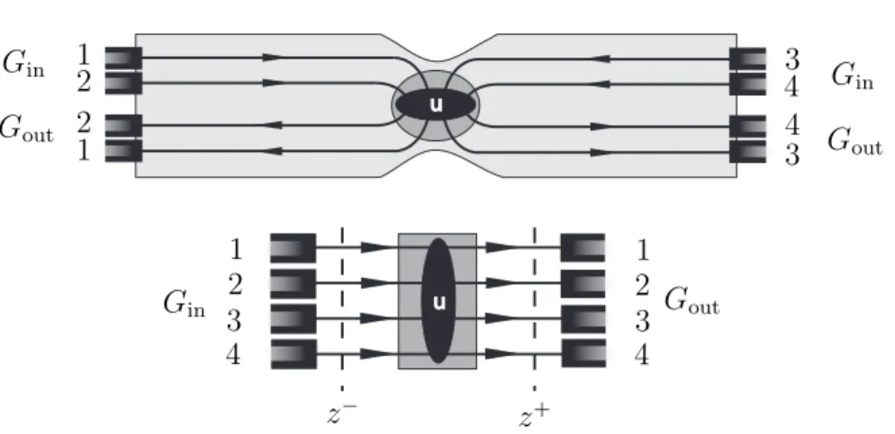
Figure 2.1. We consider a general scatterer connected to reservoirs. The top fig-ure is a diagram of one possible physical realization of a scatterer. Channels carry electrons towards and away from a scattering region (shaded dark gray) where inter-channel scattering takes place. Reservoirs are characterized by Keldysh Green functionsGin (out). These Green functions also carry a channel index, in
order to account for, among other things, voltage biasing. In setups such as the the Quantum Hall experiment where there is a Hall voltage,Ginwill differ from
Gout, while in an ordinary QPC, the two will be identical. The bottom figure
shows how the physical setup is represented in our model. Channels are unfolded so that all electrons enter atz− and leave atz+.
Hamiltonian of the scatterer to be
H=vF
X
m,n
Z
dz ψ†m(z){−iδm,n∂z+um,n(z)}ψn(z) +Hres+HT, (2.5)
where Hres represents the reservoirs, and HT takes account of tunneling
between the conductor and the reservoirs. The scattering region and the reservoirs are spatially separated. This means that the scattering potential
umn(z) is non-zero only in a region z−< z < z+ while tunneling between the reservoirs and the conductor only takes place outside this region. Note that in our model, scattering channels have been “unfolded”, so that in stead of working with a channel that confines particles in the interval
(−∞,0] and allowing for propagation both in the positive and negative directions, we equivalently work with channels in which particles propagate along(−∞,∞), but only in the positive direction. Hence, to make contact