MEAN-FIELD METHODS IN LARGE STOCHASTIC NETWORKS
Eric Friedlander
A dissertation submitted to the faculty of the University of North Carolina at Chapel Hill in partial fulfillment of the requirements for the degree of Doctor of
Philosophy in the Department of Statistics and Operations Research.
Chapel Hill 2018
ABSTRACT
ERIC FRIEDLANDER: Mean-Field Methods in Large Stochastic Networks (Under the direction of Amarjit Budhiraja)
ACKNOWLEDGEMENTS
I would like to thank all the people without whom this dissertation would not be possible. First, I would like to express my deepest gratitude and admiration for my advisor, Professor Amarjit Budhiraja, as I can’t even imagine having a better mentor. I am forever indebted to him for his patience, guidance, teaching, training, and career advice. Throughout my graduate career here at UNC, Amarjit has helped to provide ideas when I’ve been stuck and proofread both the grammar and technical details of my work. Later on, he provided invaluable career advice and helped to keep me calm while I was on the job market. Without his guiding hand I would not be as successful (or sane) as I am now. I feel lucky to have had such a wonderful advisor. Finally, I would like to thank him for all of the funding he has provided me throughout my tenure at UNC. This financial support allowed me to fully focus on my work, as well as attend a variety of conferences and workshops integral to my development as a researcher.
I would be remiss if I did not acknowledge the immense contributions of the department’s unsung heroes. Alison Kieber, Christine Keat, Sam Radel, and Linda Stutts have provided invaluable help, guidance, support, and friendship throughout my time at UNC. I would like to thank Christine for helping to organize and send out all of my recommendation letters. In addi-tion, Christine was instrumental in helping to sort out any class/scheduling related problems I ever had. This was no small undertaking and I would certainly have been unable to do it myself. Thank you to Sam and Linda for helping to organize all things business/financial related. I appreciate all of Alison’s help with organizing everything from textbooks to classrooms. Your help has been invaluable throughout my time here. Finally, I would like to thank all of you for the time you spent chatting with me. I feel that we’ve had some wonderful conversations over the years and I will truly miss spending time with all of you.
I would like to take a moment to acknowledge my undergraduate advisor Professor Rudy Guerra and his wife Nancy Guerra. It is because of Rudy that I even ended up in the field of statistics and I can honestly say that I would be a much different person if not for his advice, guidance, and friendship. Rudy remains one of the most important people in my life and one of the small group of people whose advice I constantly solicit and trust. It is unlikely that I would have made it to this point without his help. In addition, Nancy is one of the most loving and uplifting people I have ever had the pleasure to meet. While I have not tasted any of her amazing cooking in some years, I always enjoy having the opportunity to chat with her over the phone and catch up. It never fails to bring a smile to my face.
I would like to thank all of my friends. Thank you:
Mike Lamm for spending half of your weekends with me and being such a great friend. James Wilson and Rosie Scott for all of your advice, friendship, and fun times.
Jimmy Jin, Kelly Bodwin, and John Palowitch for your advice as older students.
Donqing Yu, Eunjee Lee, Samopriya Basu, Kevin O’Connor, and Sepehr Moravej for being such wonderful officemates.
Meilei Jiang and Suman Chakraborty for the homework help, discussions, and fun expe-riences we’ve had over the past five years.
Dylan Glotzer and Lindsey Comer for being such great friends. Also for performing my marriage.
Adam Waterbury, Michael Conroy, Candice Crilly, Jack Prothero, Aditya Bhalaram, Car-son Mosso, Mark He, and Mike Perlmutter for all the fun we’ve had together.
Ruoyu Wu for the insightful discussions and talks that we’ve had.
Sayan Banerjee for joking around with me and for the useful discussions we’ve had.
TABLE OF CONTENTS
LIST OF TABLES . . . x
LIST OF ABBREVIATIONS AND SYMBOLS . . . xi
1 Introduction . . . 1
1.1 Summary of Thesis . . . 2
1.1.1 Diffusion Approximations for Controlled Weakly Interacting Large Finite State Systems with Simultaneous Jumps . . . 2
1.1.2 Load Balancing Mechanisms in Cloud Storage Systems . . . 5
1.2 Notation. . . 8
2 Background and Preliminaries . . . 10
2.1 Weakly Interacting Particle Systems and Communication Networks . . . 10
2.2 Load Balancing. . . 13
2.3 Law of Large Numbers . . . 15
2.4 Diffusion Approximations . . . 16
2.5 Overview & Organization . . . 17
3 Diffusion Approximations for Controlled Weakly Interacting Large Finite State Systems with Simultaneous Jumps . . . 20
3.1 Problem Formulation and Main Results . . . 22
3.1.1 Weakly Interacting Jump Markov Process . . . 23
3.1.2 Controlled System . . . 25
3.1.3 Diffusion Control Problem . . . 27
3.1.4 Main Result . . . 31
3.2 Tightness . . . 33
3.4 Feedback Controls . . . 46
3.4.1 Feedback Control in then-th System . . . 47
3.4.2 Diffusion Feedback Control . . . 47
3.4.3 Convergence Under Continuous Feedback Controls . . . 49
3.5 Near Optimal Continuous Feedback Controls . . . 54
3.6 Example . . . 63
4 Load Balancing Mechanisms in Cloud Storage Systems. . . 70
4.1 Model Description and Main Result . . . 74
4.1.1 Supermarket Model . . . 82
4.2 Semimartingale Representation . . . 84
4.3 Fluid Limit . . . 85
4.3.1 Tightness . . . 86
4.3.2 Convergence . . . 89
4.3.3 Proof of Lemma 4 . . . 93
4.3.4 Proof of Theorem 11 . . . 95
4.3.5 Proof of Theorem 12 . . . 96
4.3.6 Proof of Theorem 13 . . . 100
4.4 Diffusion Approximation . . . 101
4.4.1 Moment Bounds . . . 101
4.4.2 Tightness . . . 107
4.4.3 Convergence . . . 115
4.5 Numerical Results . . . 124
Appendix A Tightness Criteria . . . 127
A.1 Conditions [A] and [T1] of (Joffe and M´etivier, 1986) . . . 127
A.2 Criterion for Tightness of Hilbert Space-Valued Random Variables . . . 128
A.3 Aldous-Kurtz Criterion for Tightness of RCLL Processes . . . 128
LIST OF TABLES
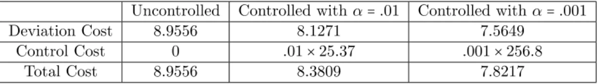
3.1 Cost over 128 Simulations . . . 68
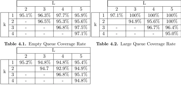
4.1 Empty Queue Coverage Rate . . . 125
4.2 Large Queue Coverage Rate . . . 125
4.3 Mean Queue Length Coverage Rate . . . 125
LIST OF ABBREVIATIONS AND SYMBOLS
JSQ Join-the-Shortest Queue JIQ Join-the-Idle Queue
MDS Maximum Distance Separable
LLN Law of Large Numbers
CLT Central Limit Theorem
ODE Ordinary Differential Equation SDE Stochastic Differential Equation FIFO First-In-First-Out
RCLL Right continuous functions (stochastic processes) with left limits
N Set of natural numbers
N0 Set of non-negative integers
R Set of real numbers
R+ Set of non-negative real numbers Rd Set of d-dimensional real vectors
Z Set of integers
B(S) Borel σ-field on a topological spaceS
Cb(S) The collection of bounded continuous functions from space S toR C([0, T] ∶S) The space of continuous functions from [0, T] toS
C(S1∶S2) The space of continuous functions from S1 toS2
Cb(S1∶S2) The space of bounded continuous functions fromS1 toS2
Ck(Rd) The space of continuous functions from Rd to R whose first k derivatives exist and are continuous
Ckc(Rd) The subset of Ck(Rd)consisting of functions with compact support
C∞(Rd) The space of continuous functions from Rd toR where all derivatives exist and are continuous
C1,2([0, T] ×Rd) The space of continuous functions from [0, T] ×Rd to Ronce continuously differentiable in the time coordinate and twice continuously differentiable in the space coordinate
B(r) The L1 ball of radiusr inRdcentered at the origin ∥ ⋅ ∥ Euclidean norm in Rd
∥f∥∞ The sup norm of a real-valued functionf (i.e. supx∈S∣f(x)∣) Sp A Linear span of a set A
Mm×n(S) The space ofm×n-dimensional matrices whose entries take values isS Tr(M) The trace of a matrixM
1 Vector of 1’s
I Identity matrix or operator (depending on context) M(S) The space of locally finite measures on Polish space S `2 The space of square summable real valued sequences
`1 The space of absolutely summable real valued sequences
∥ ⋅ ∥2 The norm of`2
∥ ⋅ ∥1 The norm of`1
⟨x, y⟩2 The inner product betweenx, y∈`2
∥A∥HS The Hilbert-Schmidt norm of Hilbert-Schmidt operatorA
M2
T(H) Space of continuous, square integrable martingalesM ≡ {M(t)}0≤t≤T taking
values in the Hilbert space HwithM(0) =0 (a)+ The positive part of a
CHAPTER 1 Introduction
“All models are wrong but some are useful!” - George Box
1.1 Summary of Thesis
1.1.1 Diffusion Approximations for Controlled Weakly Interacting Large Finite State Systems with Simultaneous Jumps
We study a pure jump, weakly interacting, Markovian particle system in which jump rates can be dynamically modulated by a controller. The stochastic system of interest describes the state evolution of a collection of nparticles where each particle’s state takes values in a finite setX. By a weak interaction we mean that the jump rates for a typical particle depend on the states of the remaining particles through the empirical distribution of particle states. System dynamics will allow for multiple particles to change states simultaneously, but there will be a fixed finite number of jump types. Such jump-Markov processes have been proposed as models for ad hoc wireless networks (Antunes et al., 2008) of the following form. Consider a system of n finite capacity servers (particles/nodes). Jobs of K different types, each with their own capacity requirement, arrive at each node at rate λk, k = 1, . . . , K and are admitted if there
is enough available capacity. All the jobs in the system of type k have exponential residence time with mean τk−1. After an exponential holding time with mean γk−1 a job of type k will attempt to switch to another server which is chosen uniformly at random, and is admitted if there is available capacity, otherwise the job is lost. The state of a particle describes the number of various types of jobs being processed at the server. Under conditions, by classical results, the stochastic process of particle state empirical measures converges to the solution of a d-dimensional ODE (cf. (Kurtz, 1970)), where d= ∣X∣. This ODE captures the nominal behavior of the system over time asn becomes large.
desired nominal behavior. In general, adjusting system parameters incurs a cost and thus there is a trade off between this and the cost for deviating from the nominal behavior. A natural approach for analyzing this trade off is through an optimal stochastic control formulation where the controller seeks to minimize a suitable cost function which accounts for both types of costs noted above.
order to nudge the system toward its nominal state. Specifically, the overall rate of jumps in the system is O(n) whereas the allowable rate controls will be O(√n). Although the magnitude of control becomes negligible compared to the overall rate as nbecomes large, in the diffusion scaling such a control can lead to an appreciable improvement in performance (see Section 3.6 for some numerical results). In the LLN limit the controlled and uncontrolled systems both converge to the same nominal behavior as expected, but the diffusion limit of the two systems will in general differ in the drift coefficient. In particular, under suitable feedback controls the centered and normalized controlled process will converge to a diffusion with a nonlinear (in state) drift term whereas the uncontrolled process will converge to a time inhomogeneous Gauss-Markov process. In terms of cost, one can consider various types of criteria, but for simplicity we restrict ourselves to a finite time horizon cost where the running cost is a sum of two terms. The first term is a continuous function, with at most polynomial growth, of the state of the centered and normalized empirical measure, and the second is a finite convex function of the (normalized) control.
value function of the limit diffusion control problem. In addition, the result states that for any
ε> 0, there exists an ε-optimal continuous feedback control and that the cost incurred from using such a control in the prelimit system will converge to the cost in the limit. What this means is that instead of solving the original control problem, one can solve a diffusion control problem. Using that solution in the original system will yield a near optimal solution if n is large.
In Section 3.6, we will illustrate our approach through a numerical example. This example is the controlled analogue of a model introduced in (Antunes et al., 2008), and one can approach more general forms of this model along similar lines. The running cost function we consider is quadratic in the normalized state and control processes. The corresponding limit diffusion control problem in this case becomes the classical stochastic linear quadratic regulator (LQR) with time dependent coefficients (see (Fleming and Rishel, 1976)). The optimal feedback control for the diffusion control problem can be given explicitly by solving a suitable Riccati equation. Our numerical results show that implementation of the control policy based on the optimal feedback control for the limit LQR to a system withn=10,000 leads to an improvement of up to 15.5% on the cost for the uncontrolled system.
1.1.2 Load Balancing Mechanisms in Cloud Storage Systems
In the world of cloud-based computing, large data centers are often used for file storage. These data centers consist of large networks of servers that are used to store even larger sets of files. In order to improve reliability and retrieval speed, these files are often “coded”. By coded, we mean that the file is broken down into smaller pieces which are stored on multiple servers. Consider the situation in which there are four servers and one file. One can store the entire file on one server but in such a configuration the file would be inaccessible if that server were to fail. In order to improve reliability, one can replicate the file across all four servers but such a method would require much more memory. Suppose we instead split the file into halves,A and
This can be accomplished using the Maximum Distance Separable (MDS) code with parameters (L, k)(Lin and Costello, 2004). The MDS code greatly improves reliability sinceL−k+1 servers must fail before the file becomes irretrievable, while only requiring enough total memory to store
L/k files. Given a coding scheme, one can consider load balancing mechanisms to improve file retrieval speed. In (Li et al., 2016), two routing schemes, called Batch Sampling (BS) and Redundant Request with Killing (RRK), are considered. In BS routing, incoming jobs are routed to the kshortest queues containing the file being requested, while in RRK routing jobs are routed to all servers containing the requested file and then removed from the queue (killed) oncekpieces of the file have been returned. The paper (Li et al., 2016) formally calculates the steady state (T → ∞) queue length distribution in the large system limit (n→ ∞) and gives simulation results for different values ofLandkin both routing schemes. In this work we focus primarily on BS routing.
We are interested in developing a rigorous limit theory for such load balancing schemes for systems with MDS coding as nbecomes large. Specifically, we establish law of large numbers and diffusion approximations for such systems under an appropriate scaling, as n→ ∞. Such limit theorems provide useful model simplifications that can then be employed for approxi-mate simulation of the large and complexn-server systems (see Section 4.5 for some numerical results). These limit theorems are also the first steps towards making rigorous the program initiated in (Li et al., 2016) of developing steady state approximations for such systems, with provable convergence properties asnbecomes large.
above formulation describes an interacting particle system withsimultaneous jumps. Note that the symmetry structure introduced above implies that every time a file request arrives, it leads to a selection of Lservers uniformly at random (from which the kservers with shortest queues are chosen). In particular this says that the well studied “Power-of-d” routing scheme (also known as the “supermarket model”) is a special case of the scheme considered here on taking
L=dandk=1. Direct analysis of such large and complex n-server systems is challenging even by simulation methods as frequently the servers in networks of interest number in the hundreds of thousands with arrival rates of file requests of similar order. The goal of this work is to develop suitable approximate approaches to such systems.
Limit theorems of the form studied in this work can be used for model simplification and for computing approximations for performance measures, e.g. through simulation methods. Direct simulation of the underlyingn-server system would in general be prohibitively expensive for large n since the jumps in the system occur at rate proportional to n. The asymptotic approximations given in this work (cf. Theorems 10 and 14) allow a system manager to simulate performance metrics for the system at a coarser scale via numerical ODE solvers or Euler discretizations for SDE (see Section 4.5 for an example). Although the systems considered here are required to satisfy certain symmetry conditions (all files are equally sized and all jobs are in equal demand), the simplified models given by the limiting ODE and SDE give useful qualitative insights into the behavior of large storage networks employing these types of coding schemes.
(Li et al., 2016), it has been shown that the queue length processQnfor the n-server system is positive recurrent and, thus, has a unique invariant probability measure. This then implies that the occupancy measure process has a unique invariant distribution. In this work we show that this invariant measure converges toδ¯u in probability, as n→ ∞. Roughly speaking, this result
says that the limits n→ ∞ and t→ ∞can be interchanged and, in particular, the fixed point of the ODE is a good approximation for the steady state behavior of the occupancy process for largen.
1.2 Notation
The following notation will be used. We will use {Xt} and {X(t)} interchangeably for
stochastic processes. The space of probability measures on a Polish spaceS, equipped with the topology of weak convergence, will be denoted by P(S). When S =N0 we will metrize P(S) with the metricd0 defined as
d0(µ, ν) ≐
∞ ∑
j=0
∣µ(j) −ν(j)∣
2j , µ, ν∈ P(N0).
ForS valued random variablesX,Xn,n≥1, convergence in distribution ofXn toX asn→ ∞
will be denoted as Xn⇒ X. The Borel σ-field on a Polish space S will be denoted as B(S). The space of functions that are right continuous with left limits (RCLL) from[0, T]toSwill be denoted asD([0, T] ∶S)and equipped with the usual Skorohod topology. SimilarlyC([0, T] ∶S) will be the space of continuous functions from[0, T]toS, equipped with the uniform topology. We will usually denote byκ, κ1, κ2,⋯, the constants that appear in various estimates within
a proof. The values of these constants may change from one proof to another. Cardinality of a finite set A will be denoted as∣A∣. We will denote byB(r)the L1 ball of radiusr centered at the origin in some Euclidean spaceRd. The Euclidean norm of ad-dimensional vector or ad×d matrix will be denoted as ∥ ⋅ ∥. The linear span of a set A⊂Rd will be denoted as SpA. The space of continuous (resp. continuous and bounded) functions from metric spaceS1 toS2 will be
and are continuous will be denoted Ck(Rd) (resp. C∞(Rd)). We denote the subset of Ck(Rd) of functions with compact support asCkc(Rd). SimilarlyC1,2([0, T] ×Rd) denotes the space of
functions from(0, T)×RdtoRthat are once continuously differentiable in the time coordinate, twice continuously differentiable in the space coordinate, and are such that the function and its derivatives can be continuously extended to [0, T] ×Rd. The space of m×n-dimensional matrices whose entries take values in a setSwill be denotedMm×n(S). ForM ∈Mm×n(S),Mi,j
will the denote that entry ofM which is in thei-th row andj-th column. The transpose of a matrixM will be denoted as M′ and trace of a square matrixM will be denoted as Tr(M). 1
andI will denote the vector of 1’s and the identity matrix, respectively, the dimension of which will be context dependent. For a Polish space S we denote by M(S) the space of all locally finite measures on S. This space will be equipped with the usual vague topology, namely, the weakest topology such that for everyf ∈Cb(S)with compact support,
ν↦ ∫
S
f(u)ν(du), ν∈ M(S),
is continuous.
Let`2= {(aj)∞j=0∣ ∑∞j=0a2j < ∞}be the space of square summable real sequences. This space
is a Hilbert space with inner product
⟨x, y⟩2=
∞ ∑
j=0 xjyj.
We denote the corresponding norm as ∥ ⋅ ∥2. Similarly, `1 = {(aj)∞j=0∣ ∑∞j=0∣aj∣ < ∞} and ∥ ⋅ ∥1
is the norm on this Banach space. The Hilbert-Schmidt norm of a Hilbert-Schmidt operator
A on `2 will be denoted ∥A∥HS (cf. Appendix B). We denote by I the identity operator. For
a Hilbert SpaceH,M2T(H) will denote the space of allH-valued continuous, square integrable
martingales M ≡ {M(t)}0≤t≤T, such that M(0) =0. For a real number a, (a)+ will denote the
CHAPTER 2
Background and Preliminaries
This chapter contains an introduction to some models used for a variety of communication networks as well as some background on the techniques used to analyze them. In addition, we review some of the related literature on communication networks and weakly interacting particle systems. In Section 2.1, we present an overview of some of the relevant existing work on weakly interacting particle systems in communication networks. These works describe some of the ways in which weakly interacting particle systems are used in modeling communication networks and why such models are useful. Specifically, weakly interacting particle systems suggest simpler models through mean field approximations under certain symmetry conditions on the system. The mean field techniques described are particularly useful for load balancing problems. Section 2.2 is devoted to an overview of the existing relevant work in this area. In Section 2.3, we present a LLN result which can be used to approximate the dynamics of a given system through a set of ODE. Section 2.4 provides an introduction to methods for analyzing the deviations around the LLN. Namely, we provide some of the basic approaches to proving various Central Limit Theorems (CLT) of interest. These approximation techniques allow us to analyze communication networks whose large size make this analysis otherwise intractable. Section 2.5 provides an outline of topics in this dissertation
2.1 Weakly Interacting Particle Systems and Communication Networks
the evolution of a typical particle’s state only depends on its own current state and the current empirical measure of the states of all particles in the system. In other words, the dynamics of a given particle only depends on the total number of particles in each state and not on the state of any individual particle (other than itself). This property, together with certain natu-ral symmetry conditions, implies the exchangeability of the system that makes these networks well-suited for mean field approximations. More specifically, if one views the evolution of the system through the empirical measure of particle states, then, under conditions, the system can be approximated by a deterministic evolution equation in the space of probability measures, referred to as the Mckean-Vlasov equation. Under conditions, one can also establish a CLT that says that the appropriately scaled fluctuations from this nominal deterministic evolution equation converge to a Gaussian process which is described through a linear SDE (Shiga and Tanaka, 1985; Sznitman, 1991). These fluid and diffusion approximations can be used to ana-lyze useful properties regarding the system (e.g. performance measures, stability, etc.). Below we discuss several examples of such networks that have been studied in the literature.
In (Gibbens et al., 1990), the authors study a routing scheme used in telecommunication networks called Random Alternative Routing. The authors analyze how this method performs on calls routed along the edges of a complete graph withnnodes. In this setting, the “particles” are the links between the nodes rather than the nodes themselves. Each link can handle a fixed, maximum number of calls at a given time. A natural way to view the state of the system is through the available capacity at each link. It is assumed that calls arrive at each link as a Poisson process and are routed as follows. If a call attempts to use a link which does not have available capacity, two more links are chosen uniformly at random and, if there is available capacity at both, the call is routed through that path, otherwise the call is lost. The authors derive a LLN approximation for the system (asn→ ∞) and show that the limit ODE has exactly two fixed points. In addition, a diffusion approximation is presented and used to explore the tunneling behavior between the two stable points.
The paper (Hunt and Kurtz, 1994) presents a method of analyzing large loss networks. Specifically, the authors consider a network with J links. Each link j has Cj “circuits”. In
in (Gibbens et al., 1990), namely the paper considers the limit as the arrival/departure rates and the available capacity go to infinity rather than as the number of links in the network approach infinity.
In (Antunes et al., 2008), a general mathematical model for a class of communication networks is studied. Consider a collection of particles (or nodes) each with a finite amount of space (or capacity). Different types of jobs, each with its own capacity requirement, arrive from the outside and are accepted only if there is sufficient capacity to meet the job’s requirement. After an exponential holding time, jobs can either move to another particle or leave the system. The evolution of the available capacity at all nodes in the system can be described through a high dimensional pure jump Markov process. Similar to (Gibbens et al., 1990), the authors present a LLN approximation of the empirical measure process associated with the system and then show that the resulting deterministic system of ODEs has multiple stable points.
Weakly interacting particle systems are a tractable class of models since they can be often approximated by simpler mean field models. One such approximation result, which is closely related to the LLN results described above, has been established in (Graham, 2000) that studies a class of routing schemes for large queuing networks. A sequence of infinite collections of sequences ofS-valued random variables is said to beQ-chaotic, whereQis a probability measure on S, if the joint probability law of any subcollection of sequences of k random variables converges to Q⊗k for all k ≥ 1. Namely, the collection of random variables is asymptotically i.i.d. with probability law Q. Consider a collection of n servers which process jobs at rate
µ from their own infinite buffer queues. Jobs arrive in the system at rate λn and each job is immediately routed to the shortest of d randomly chosen queues. It is shown in (Graham, 2000) that, under exchangeability conditions and independence of initial conditions, this system has a “Propagation of Chaos” (initial independence [i.e. chaos of particle states] propagates to later time instants) property. Namely the queue length processes viewed as a collection of D(R+ ∶N0)-valued random variables are Q-chaotic for an appropriate probability measure Q
onD(R+∶N0) whereD(R+∶N0)is the space of right continuous functions with left limits from
R+ toN0 equipped with the usual Skorohod topology.
exchangeable, the random variables can be divided intoK classes such that there is exchange-ability within each class. Stated formally, a system is said to beQ1⊗ ⋯ ⊗ QK-multi-chaotic if
the joint probability law of any collection ofKmvariables, such that mare selected from each exchangeable group, converges toQ⊗1m⊗⋯⊗Q⊗Km. The authors establish such a multi-chaoticity property for a class of queueing systems. Using this result they then analyze a model for data transmission.
2.2 Load Balancing
Due to the need to properly design and maintain distributed processor networks and cloud-based storage systems, mechanisms for an efficient allocation of jobs or file requests in such networks has garnered quite a bit of attention in recent years. A typical model of interest is described in terms of asystem of n processors or servers each maintaining its own FIFO queue. A stream of jobs or file requests enters the system and are routed by a centralized dispatcher into one or more of the queues. Ultimately the goal is to study how different routing schemes impact various performance metrics of interest (e.g. mean delay time, queue length distribution, etc.). This class of problems associated with different types of routing schemes is frequently referred to as load balancing. In general, the large size of such networks precludes a direct analysis of such systems so the performance is typically studied in a suitable asymptotic regime. In many settings, by appropriately scaling the system and taking limits (e.g. as the number of servers n tends to infinity), one can establish fluid or diffusion approximations for the desired performance metrics. I now give a brief review of some relevant work but refer the interested reader to (van der Boor et al., 2017) for a more in depth exposition.
The simplest load balancing scheme is random routing. Namely, when a job arrives in the system, the dispatcher sends it to a server which is chosen uniformly at random. Consider the expectation of the empirical measure of queue lengthsπn under the stationary distribution. It can be shown that as n→ ∞, if the traffic intensity λ (i.e. the ratio of arrival and departure rates) is less than one, the limiting expectation, which is a deterministic measure onN0 denoted
analyzed the so-called Power-of-d routing scheme (also known as the Supermarket Model). Under this scheme, at each instant of job arrival, the dispatcher polls d randomly chosen servers and routes the jobs to the server with the shortest queue. The paper (Graham, 2000) establishes a functional law of large numbers forπn on D([0, T] ∶ S) in the Power-of-drouting scheme using characterization results for nonlinear martingale problems. In (Graham, 2000; Vvedenskaya et al., 1996; Mitzenmacher, 2001), it is shown that for d≥ 2 the corresponding measure ν has tails which decay hyperexponentially, namely ν[k,∞) ∼ λ(dk−1)/(d−1), which is a vast improvement over the exponential rate for the setting where jobs are routed to servers uniformly at random.
In (Eschenfeldt and Gamarnik, 2015), the authors consider another routing scheme known as Join-the-Shortest Queue (JSQ) in which incoming jobs are simply routed into the shortest available queue. This scheme corresponds to the Power-of-dupon takingd=n. However, sinced
scales withnthe asymptotic analysis is quite different. The authors establish fluid and diffusion approximations for the empirical measure JSQ routing policy in the large-system limit under a heavy-traffic scaling. It is shown that probability of having a queue of length larger than one converges to zero asn→ ∞. Furthermore, the diffusion limit can be characterized through a two-dimensional diffusion. It follows from this theorem that JSQ produces, asymptotically, the minimal possible wait time. Namely, as the number of servers increases to infinity and the traffic intensity approaches criticality, the proportion of servers with two of more jobs goes to zero and thus all jobs which enter the system are routed to empty servers. The excellent performance of JSQ is counterbalanced by an extremely high overhead cost. The dispatcher must query every server each time a jobs arrives which may be costly in large networks in which jobs are arriving extremely rapidly.
between push and pull based schemes is subtle, but by using pull based schemes one can reduce communication overhead while maintaining low wait times. In the JIQ scheme each server needs to communicate to the dispatcher when its buffer is empty. In practice this implies that the number of communications between the dispatcher and the server is of the same order as the total number of arrivals in the system and thus, in terms of communication costs JIQ and JSQ are not very different. The authors of (Mukherjee et al., 2016b) also establish a useful interchange of limits property showing that the steady-state behavior of the n-server system converges to the unique fixed point of the limiting system under a fluid scaling.
While not discussed here we refer the interested reader to (Mitzenmacher, 2001; Bramson et al., 2012; Stolyar, 2015; Graham, 2000; Mukherjee et al., 2016a, 2017) and references therein for further work on load balancing. In the next two sections we summarize the basic LLN and central limit theorems for pure jump Markov processes that are useful for studying asymptotics of weakly interacting particle systems of the form considered in this work.
2.3 Law of Large Numbers
Typically, the first method employed when attempting to describe the evolution of the systems of interest here, as their size becomes large, is to derive a LLN limit for the associated empirical measure. This limit is given in terms of a system of coupled ODE and describes the asymptotic behavior of the system under a fluid scaling. One of the classical works on such limit theory is (Kurtz, 1970) which proves the following result (see Theorem 2.11 therein):
Theorem 1. Let E be a closed set in Rk and let, forn∈N, En=E∩n1Nk0. Let {µn(t)}t≥0 be a pure jump Markov process with state space En and infinitesimal generatorAn, defined as
Anf(x) =λn(x) ∫
En[f(z) −f(x)]γn(x, dz)
where λn∶En→R+ and γn is a transition probability kernel onEn. Define
Fn(x) =λn(x) ∫
En(z−x)γn(x, dz). (2.1)
i) There exists a Lipschitz function F∶Rk→RK such that
lim
n→∞xsup∈En∣Fn(x) −F(x)∣ =0.
ii) limn→∞µn(0) =x0 for some x0∈E.
Let µ be the solution to the following ODE
˙
µ(s) =F(µ(s)), µ(0) =x0.
Then for every δ>0 and t>0
lim
n→∞P{sups≤t ∣µn(s) −µ(s)∣ >δ} =0.
This theorem says that for a sequence of K-component jump Markov processes, if the functionFnin (2.1) obtained from the generator of the process converges in a suitable manner,
then the sequence of processes converge to the solution of a system of ODE. To see how this result applies to weakly interacting systems note that for a typical sequence of communication networks considered in our work the n-th state process is n-dimensional. In particular the dimension of the state space is increasing withn. In order to arrive at a sequence of processes with a common state space we instead view the system through its empirical measure process which will have a finite state space if each particle’s state space is finite. In our work we will usually apply Theorem 1 (or a generalization in the case that the state space is countably infinite) to this empirical measure process. In general, an empirical measure process constructed from an n-dimensional Markov process may not itself be Markovian. However, under the symmetry properties of the models considered in this work, the Markov property of the empirical process will indeed hold which will allow the use of Theorem 1.
2.4 Diffusion Approximations
interested in the asymptotic behavior of the stochastic processVndefined as
Vn(t) =√n(µn(t) −µ(t)), t≥0.
Under conditions, this asymptotic behavior can be characterized in terms of a suitable diffusion process. One natural approach for proving such a limit theorem is to describe the evolution of the centered and scaled process Vn through a collection of appropriate time changed Poisson
processes (see e.g. (3.6) in Chapter 3). Using this description, one can give a semimartingale representation forVn of the following form
Vn(t) =Vn(0) + ∫ t
0 An(s, Vn(s))ds+Mn(t) +op(1)
where Mn is a local martingale with respect to a suitable filtration andAn∶ [0,∞) ×Rk→Rk is a suitable map.
The first key step in proving the convergence to a diffusion process is to argue tightness of (Vn, Mn). Next, one needs to argue that every weak limit point (V, M) satisfies a stochastic
equation of the form
V(t) = ∫
t
0 a(s, V(s))ds+M(t), M(t) = ∫
t
0 σ(s)dB(s), (2.2)
wherea, σ are suitable maps, B is a Brownian motion with respect to a suitable filtration and
V is a continuous process adapted to the filtration. The final step is to argue the uniqueness of solutions to the stochastic equation (2.2). This progression of arguments can be carried out under quite general conditions on the model (see e.g. (Joffe and M´etivier, 1986)).
2.5 Overview & Organization
state. We consider a formulation where the system manager, by adjusting various rates, can nudge the actual stochastic system closer to the desired nominal state. However, exercising control of rates incurs a cost and one needs to suitably balance this cost with the cost of deviating from the desired behavior. Theory of stochastic control gives a natural framework for analyzing such processes. For large systems, solving such stochastic control problems directly is intractable. In this work, we instead consider an approximate approach. Specifically, we introduce a diffusion control problem which approximates the control problem of interest under a suitable scaling. Such diffusion control problems have been well studied and there exists an extensive literature on numerical methods for finding solutions (see e.g. (Kushner and Dupuis, 2013)). Our main result (Theorem 2) shows how an analysis of this diffusion control problem leads to construction of an asymptotically optimal control policy for the system of interest. A paper (Budhiraja et al., 2018) has appeared in the Annals of Applied Probability.
CHAPTER 3
Diffusion Approximations for Controlled Weakly Interacting Large Finite State Systems with Simultaneous Jumps
In this chapter we study a pure jump, weakly interacting, Markovian particle system in which jump rates can be dynamically modulated by a controller. The stochastic system of interest describes the state evolution of a collection of n particles where each particle’s state takes values in a finite setX. In many applications, the jump rate of such a system scales with
particle system such that the associated costs converge to the cost under the feedback policy for the diffusion control problem (Theorem 7). We begin, in Theorem 8, by arguing that for the diffusion control problem the infimum over all admissible controls is the same as that over the class of feedback controls. Proof of this proceeds via certain conditioning arguments and PDE characterization results (cf. (Borkar, 1989)) that allow the construction of a feedback control associated with any given admissible control such that the cost corresponding to the feedback control is no larger than that of the given admissible control. The result says that one can find an ε-optimal control in the space of feedback controls. Although any such control corresponds to a natural collection of control policies for the sequence of n-particle systems, in order to prove the convergence of associated costs, which once more is based on martingale problem methods, we require additional regularity properties of the feedback control. The key step is Theorem 9 that shows that for any feedback control g there exists a sequence of continuous feedback controls{gn}for the limit diffusion control problem such that the associated sequence
of controlled diffusions converge weakly to the diffusion under the feedback controlg. The proof requires some estimates based on an application of Girsanov’s theorem which, in turn, relies on the non-degeneracy of the diffusion coefficient. Although the controlled diffusion that describes the asymptotic model is degenerate, we show that there is an equivalent formulation in terms of a (d−1)-dimensional controlled diffusion which is uniformly non-degenerate under suitable assumptions. This equivalent representation, in addition to providing a feedback control of the desired form, is also key in proving weak uniqueness for SDE describing limit state processes associated with feedback controls.
also introduce our main assumptions on the controlled rate functions (Conditions 3.1.3 and 3.1.4). In Section 3.1.4 we present our main result, namely Theorem 2. In order to validate the results of this chapter, we present a numerical example in Section 3.6. This example is the controlled analogue of a model introduced in (Antunes et al., 2008). The running cost function we consider is quadratic in the normalized state and control processes. The corresponding limit diffusion control problem in this case becomes the classical stochastic LQR with time dependent coefficients (see (Fleming and Rishel, 1976)). The remainder of the chapter is devoted to proof of Theorem 2. In Section 3.2 we present a key tightness result which is used both in the proof of the upper and lower bound. In Section 3.3 (see Theorem 3) we prove the lower bound that was discussed earlier. In preparation for the proof of the upper bound, we introduce the class of feedback controls in Section 3.4. Sections 3.4.1 and 3.4.2 describe such controls for the prelimit system and the limit diffusion model, respectively. Section 3.4.3 constructs a sequence of prelimit control policies from an arbitrary continuous feedback control for the diffusion control problem such that the cost for the particle systems under the sequence of control policies converges to the cost of the corresponding controlled diffusion. Finally in Section 3.5, we show that the infimum of the cost for the limit diffusion over all admissible controls is the same as that over the class of feedback controls and that there exist continuous feedback controls which are ε-optimal. The results from sections 3.3, 3.4, and 3.5, (namely Theorems 3, 7, and 9) together give our main result, Theorem 2.
3.1 Problem Formulation and Main Results
can be used to construct a sequence of control policies for the particle system in Section 3.1.2 that are asymptotically near optimal. For a numerical example that illustrates the application of the result, we refer the reader to Section 3.6 where we present a model from communication networks that is a controlled version of some models introduced in (Antunes et al., 2008) and which falls within the framework considered here.
3.1.1 Weakly Interacting Jump Markov Process
Fix T ∈ (0,∞). All stochastic processes in this chapter will be considered on the time horizon [0, T]. Consider a system of n particles where the state of each particle takes values in the set X = {1, . . . , d}. The evolution of the system is described by an n-dimensional pure jump Markov process Xn(t) = {Xn1(t), . . . , Xnn(t)} whereXni(t)represents the state of particle
iat time t. The system allows multiple particles to change state at a given time, but restricts such jumps toK transition types; in particular thek-th transition type can only affect at most
nk particles, k ∈ K ≐ {1, . . . , K}. The jump intensity is state dependent, however the state
dependence is of the following specific form: Denoting for x ∈ Xn, the probability measure {1
n∑ n
i=11{xi}(m)}m∈X on Xby{ζ
m
n(x)}m∈X, the jump intensity at the instant tis a function of
ζn(Xn(t)). The set of jumps and the corresponding transition rates can be described in terms
of the subset Mn of Md×d(N0) consisting of all matrices with zeroes on the diagonal and with
sum of all entries at mostn, as follows. To anyk∈Kwe associate a map Ψnk∶ P(X) ×Mn→R+ such that forx∈Xn, Ψkn(ζn(x),Θ) =0 if
∑
i,j
Θi,j >nk or d
∑
j=1
Θi,j >nζni(x), i=1, . . . , d. (3.1)
Roughly speaking, Ψkn(ζn(x),Θ) will give the rate of typek jumps (associated with Θ) when
the system is in state x ∈ Xn. A type k jump associated with Θ ∈ Mn corresponds to Θij
particles simultaneously jumping from state i to state j, for all i≠j and i, j =1, . . . , d. Thus the first inequality in (3.1) says that at mostnk particles change states under a jump of typek,
Θ, when the system is in state x∈Xn, is given as
Ψkn(ζn(x),Θ) d
∏
m=1
( nζnm(x)
∑d
j=1Θm,j)( ∑ d j=1Θm,j
Θm,1, . . . ,Θm,d)
and such a jump takes a statex∈Xnto a state ˜x∈Xnwhere
nζnm(x˜) =nζnm(x) +
d
∑
i=1
Θi,m− d
∑
j=1
Θm,j, m=1, . . . , d.
A more convenient description of this system is given through the pure jump Markov process {µn(t)} where µn(t) ≐ζn(Xn(t)) represents the empirical measure of the particle states. We
will identify the space of probability measures, P(X), with the d-dimensional simplex, S ≐ {(x1, . . . , xd) ∈Rd+∣ ∑di=1xi=1}. Similarly, we will identifyPn(X), the space of allµ∈ P(X)such thatµ{j} ∈ n1Nfor all j∈X, with Sn= S ∩n1Nd. Let, for k∈K,
∆k≐ {(I, J) ∈Nd0×Nd0∶ ∑
x∈X
Ix= ∑ x∈X
Jx≤nk, ∑ x∈X
∣Jx−Ix∣ >0},
and for ν= (I, J) ∈∆k let
Φ(ν) =Φ(I, J) ≐⎧⎪⎪⎨⎪⎪
⎩Θ∈Mn∣
d
∑
j=1
Θi,j =Ii, d
∑
i=1
Θi,j=Jj, i, j=1,⋯, d⎫⎪⎪⎬⎪⎪
⎭.
The jumps of{µn(t)}are described as follows. For eachk∈Kandν= (I, J) ∈∆kthe empirical
measure jumps fromr↦r+1neν with rate
¯
Γnk(r, ν) ≐ ∑ Θ∈Φ(ν)
Ψkn(r,Θ)
d
∏
m=1
( nrm ∑d
j=1Θm,j)( ∑ d j=1Θm,j
Θm,1, . . . ,Θm,d)
wherer= (rm)dm=1 ∈ Sn,eν ≐ ∑x∈X(Jx−Ix)ex andex is the unit vector inRdwith 1 at thex-th coordinate and 0 everywhere else. Thus a jump associated withk∈Kand ν∈∆k corresponds to Ix particles in state x, x ∈ X, simultaneously jumping to new states such that Jy of the
µn(t) is through its infinitesimal generator which is given as
¯
Lnf(r) = ∑
k∈Kν∑∈∆k
¯
Γnk(r, ν) [f(r+1
neν) −f(r)], r∈ Sn. (3.2)
We will make the following assumption on the asymptotic behavior of the rates.
Condition 3.1.1. For all k∈Kandν∈∆k there exists a Lipschitz functionr↦Γk(r, ν) onS such that
lim sup
n→∞
sup
r∈Sn
∣n1Γ¯k
n(r, ν) −Γk(r, ν)∣ =0 (3.3)
We now present a classical law of large numbers result that characterizes the limit, µ(t), of the pure jump Markov process µn(t) asn→ ∞. For a proof we refer the reader to Theorem
2.11 of (Kurtz, 1970).
Proposition 1. Define,
F(r) ≐ ∑
k∈Kν∑∈∆k
Γk(r, ν)eν, r∈ S. (3.4)
Suppose thatµn(0) →µ0 in probability and Condition 3.1.1 holds, then µn(t) →µ(t) uniformly
on[0, T], in probability, where µ(t) is the unique solution of the ODE
˙
µ(t) =F(µ(t)), µ(0) =µ0. (3.5)
3.1.2 Controlled System
In this chapter we will study a controlled version of the Markov process introduced in Section 3.1.1. Roughly speaking, control action will allow perturbations of the rate function ¯
Γkn that are of O (√1n). The goal of the controller is to minimize a suitable finite time horizon cost. A precise mathematical formulation is as follows. Let
`≐ ∑
k∈K
Λ be a compact convex subset of R`, and Λn = √1nΛ for n ∈ N. Λn will be the control set
in the n-th system. Let {Γnk(r, u, ν) ∶ r ∈ Sn, u ∈ Λn, k ∈ K, ν ∈ ∆k} be a collection of
non-negative real numbers. More precisely,(r, u) ↦Γnk(r, u, ν)is a map from Sn×ΛntoR+for each
n∈N, k ∈K, ν ∈∆k. These correspond to the controlled rates in the n-th system. We now introduce the controlled stochastic processes associated with such controlled rates.
Fix n ∈ N and let (Ωn,Fn,Pn) be a probability space on which are defined unit rate mutually independent Poisson processes{Nk,ν, k ∈K, ν ∈∆k}. The processes {Nk,ν} will be
used to describe the stream of jumps corresponding to k∈K, ν ∈∆k. LetUn be a Λn-valued
measurable process representing the rate control in the system. Under control Un the state processµn(⋅) is given by the following equation:
µn(t) =µn(0) +
1
nk∑∈Kν∑∈∆k
eνNk,ν(∫ t
0 Γ
k
n(µn(s), Un(s), ν)ds). (3.7)
In order for such a control to be admissible it should satisfy suitable non-anticipative proper-ties. More precisely, Un is said to be an admissible control if, with some filtration {Ftn} on (Ωn,Fn,Pn),Un is{Ftn}-progressively measurable, µn is {Ftn}-adapted, and {Mk,νn , k ∈K, ν∈
∆k} defined below are{Ftn}-martingales
Mk,νn (t) ≐ 1
n(Nk,ν(∫
t
0 Γ
k
n(µn(s), Un(s), ν)ds) − ∫ t
0 Γ
k
n(µn(s), Un(s), ν)ds) (3.8)
with quadratic variation processes ⟨Mk,νn , Mkn′,ν′⟩t = δ(k,ν),(k′,ν′) 1
n2 ∫
t
0 Γ
k
n(µn(s), Un(s), ν)ds
where δα,α′ equals 1 if α = α′ and 0 otherwise. We note that in general such a filtration
will depend on the control. We denote the set of all such admissible controls as An.
For aUn∈ An, define the process
Vn(s) =√n(µn(s) −µ(s)) (3.9)
where, as above,µnis the state process under controlUn. We consider a cost that is a function
horizon cost” associated with an admissible controlUn∈ An and initial condition xn as,
Jn(Un, vn) ≐E∫
T
0 (k1(Vn(s)) +k2(
√
nUn(s)))ds (3.10)
where vn = √n(xn−µ0), k2 ∈ C(Λ) is a nonnegative convex function, and k1 ∈ C(Rd) is a nonnegative function with at most polynomial growth. I.e. there exists ap>1 andCk1 ∈ (0,∞)
such thatk1(x) ≤Ck1(1+ ∥x∥
p) for allx∈
Rd. Define the corresponding value function to be
Rn(vn) ≐ inf Un∈A
n
Jn(Un, vn).
Computing an optimal control for the above problem for a givennis, in general, challenging and computationally intensive. It is therefore of interest to consider approximate approaches. In the next section we introduce some conditions on the controlled rate matrices that will suggest a natural diffusion approximation for this control problem.
3.1.3 Diffusion Control Problem
We now introduce our main assumptions on the controlled rate matrices. The first two conditions make precise the requirement that controlled rates are O (√1n)perturbations of the nominal values given through {Γk, k ∈K}. In particular, the first condition will ensure that the controlled pure jump Markov process will converge to the same limit as the uncontrolled processµn in Section 3.1.1 under the law of large number scaling.
Condition 3.1.2. With{Γk(r, ν), k∈K, ν∈∆k, r∈ S}as in Condition 3.1.1
lim sup
n→∞
sup
r∈Sn
sup
u∈Λn
∣n1Γnk(r, u, ν) −Γk(r, ν)∣ =0. (3.11)
We next introduce a strengthening of Condition 3.1.2 that will play a key role in the proof of tightness of the sequence{Vn} of controlled state processes.
Condition 3.1.3. There exists aC1∈ (0,∞) such that for everyn∈N
sup
u∈Λn
sup
ξ∈Sn(y)
√
n∣1 nΓ
k n(
1 √
ny+ξ, u, ν) −Γ
k(ξ, ν)∣ ≤C
for all k∈K, ν∈∆k, and y∈B(2√n) ⊂Rd whereSn(y) = {ξ∈ S ∶√1ny+ξ∈ Sn}.
Taking y =0 in (3.12) we see that Condition 3.1.3 implies that there exists a C2 ∈ (0,∞)
such that
sup
n≥1
sup
r∈Sn
sup
u∈Λn
1
nΓ
k
n(r, u, ν) ≤C2 (3.13)
for all k∈K, ν∈∆k. Note also that Condition 3.1.3 implies Condition 3.1.2.
The next condition will identify the drift term in our limit diffusion control problem. Note that anyu∈Λ (or Λn) can be indexed byk∈Kandν∈∆kand we will denote the corresponding
entry by uk,ν.
Condition 3.1.4. There exist, for each k∈K, ν ∈∆k, bounded functions hk1(ν,⋅) ∶ S →R and
hk2(ν,⋅) ∶ S →Rd such that foru∈Λ, ξ∈ S,y∈Rd, with
Hk(y, ξ, u, ν) ≐hk1(ν, ξ)uk,ν+hk2(ν, ξ) ⋅y,
we have for all compactA⊂Rd,
lim sup
n→∞
sup
u∈Λ
sup
y∈A
sup
ξ∈Sn(y)
∣βkn(y, ξ, u, ν)∣ =0 (3.14)
where forn∈N, k∈K, and ν∈∆k, we define βkn(⋅,⋅,⋅, ν) ∶Rd× S ×Λ→R as
βkn(y, ξ, u, ν) ≐√n(1 nΓ
k n(
1 √
ny+ξ,
1 √
nu, ν) −Γ
k(ξ, ν)) −Hk(y, ξ, u, ν),
ifξ∈ Sn(y) and 0 otherwise.
Define η∶ [0, T] ×R`→Rdand β∶ [0, T] →Rd×d as
η(t, u) ≐ ∑
k∈Kν∑∈∆k
(hk1(ν, µ(t))uk,ν)eν and β(t) ≐ ∑ k∈Kν∑∈∆k
eν[hk2(ν, µ(t))]′ (3.15)
Note that
∑
k∈Kν∑∈∆k
Leta∶ [0, T] →Rd×d be defined as
a(t) ≐ ∑
k∈Kν∑∈∆k
(Γk(µ(t), ν))eνe′ν.
The d×dmatrixa(t) will be the square of the diffusion coefficient for the limit controlled diffusion process. Note that a(t) is a singular matrix sinceeν⋅1=0 for allk∈Kand ν∈∆k.
LetQ= [q1. . . qd], qk∈Rd,be ad×dorthogonal matrix (i.eQQ′=Q′Q=I) such thatqd= √1d1.
Then, in view of the above observation,
Q′a(t)Q=
⎛ ⎜⎜ ⎝
α(t) 0
0 0
⎞ ⎟⎟ ⎠
(3.17)
where α(⋅) is a Lipschitz, nonnegative definite, (d−1) × (d−1) matrix valued function. Let
α1/2(t) be the symmetric square root of α(t). Since t ↦α(t) is continuous so is t↦α1/2(t)
(see e.g. (Chen and Huan, 1997)). Define
σ(t) ≐Q⎡⎢⎢⎢
⎢⎢ ⎣
α1/2(t) 0
0 0
⎤⎥ ⎥⎥ ⎥⎥ ⎦
Q′. (3.18)
The main goal of this paper is to show that an optimal control problem for certain diffusion processes can be used to construct asymptotically near optimal control policies for the sequence of controlled systems in Section 3.1.2. We now introduce this diffusion control problem. Let (Ω,F,P,{Ft}) be a filtered probability space with a d-dimensional {Ft}-Brownian motion
{Wt}. We refer to (Ω,F,P,{Ft},{Wt}) as a system and denote it by Ξ. Denote the collection
of Ft-progressively measurable, Λ valued processes as A(Ξ). This collection will represent the
set of admissible controls for the diffusion control problem. The initial condition v0 for our
controlled diffusion process will lie in the set Vd−1 = {x ∈ Rd∣x⋅1 = 0}. For U ∈ A(Ξ) and
v0∈Vd−1, let V be the unique pathwise solution of
V(t) =v0+ ∫
t
0 η(s, U(s))ds+ ∫
t
0 β(s)V(s)ds+ ∫
t
where η, β are as introduced in (3.15) and σ is as in (3.18). Define the cost associated with
U ∈ A(Ξ) and v0∈Vd−1 as
J(U, v0) ≐E∫
T
0 (k1(V(s)) +k2(U(s)))ds. (3.20)
The value function associated with the above diffusion control problem is
R(v0) ≐inf
Ξ U∈A(infΞ)J(U, v0),
where the outside infimum is taken over all possible systems Ξ.
Although the matrixσ(t) is singular for eacht, the following condition will ensure that the dynamics ofV restricted to a certain(d−1)-dimensional subspace is non-degenerate.
Condition 3.1.5. There exists a∆∗⊂ ∪k∈K∆k such that Sp{eν ∶ν∈∆∗} equals Vd−1, and for
everyν∈∆∗ there is akν ∈Ksuch thatν ∈∆kν and
κ(T) ≐ inf
ν∈∆∗0≤inft≤TΓ
kν(µ(t), ν) >0.
The following lemma shows that under Condition 3.1.5, α is uniformly non-degenerate on compact sets.
Lemma 1. Under Condition 3.1.5, {α(t) ∶t∈ [0, T]}is a uniformly positive definite collection, namely, there exists aC(T) ∈ (0,∞)such thatx′α(t)x≥C(T)∥x∥2for allx∈Rd−1and0≤t≤T.
Proof. We first show that the matrix G= ∑ν∈∆∗eνe′ν satisfies, for some CG∈ (0,∞),
ξ′Gξ≥CG∥ξ∥2 (3.21)
for all ξ∈Vd−1. For this it satisfies to check that for any nonzeroξ∈Vd−1,ξ′Gξ>0.
Suppose for some nonzero ξ ∈Vd−1, ξ′Gξ =0. Since ξ′Gξ = ∑ξ∈∆∗∣ξ⋅eν∣2 and Sp{eν ∶ν ∈ ∆∗} =Vd−1, we must haveξ ⊥Vd−1. But by assumptionξ is a nonzero element of Vd−1 which
Now forx∈Rd−1, letting ˆx= (x0) ∈Rd,
x′α(t)x=xˆ′Q′a(t)Qxˆ= (Qxˆ)′a(t)(Qxˆ).
Since 1=√dqd and ˆxd=0,
Qxˆ⋅1= (q1x1ˆ + ⋯ +qdxˆd) ⋅1= (q1x1+ ⋯ +qd−1xd−1) ⋅1=0.
Thusy=Qxˆ∈Vd−1, and consequently fort∈ [0, T],
y′a(t)y= ∑
k∈Kν∑∈∆k
(Γk(µ(t), ν))y′eνe′νy
≥ ∑
ν∈∆∗
(Γk(ν)(µ(t), ν))y′eνe′νy≥κ(T)y′Gy≥κ(T)CG∥y∥2.
Thus
x′α(t)x≥κ(T)CG∥Qxˆ∥2=κ(T)CG∥xˆ∥2=κ(T)CG∥x∥2 (3.22)
and the result follows.
Sincet↦α(t)is Lipschitz, it follows from Lemma 1 that under Condition 3.1.5,t↦α1/2(t)
is Lipschitz as well (see Theorem 5.2.2 in (Stroock and Varadhan, 2007)). Note from (3.22), thatx′α1/2(t)x≥ (κ(T)CG)1/2∥x∥2 for all x∈Rd×dand t∈ [0, T]. In particular
sup
0≤t≤T∥
α−1/2(t)∥ < ∞. (3.23)
3.1.4 Main Result
We now present the main result of this chapter. In Section 3.4 we will show that for every measurable function g ∶ [0, T] ×Rd → Λ there exists a system Ξ and a Ug ∈ A(Ξ) such that
generator
Lgf(t, x) ≐ ∇f(x) ⋅ [η(t, g(t, x)) +β(t)x] +
1
2Tr(σ(t)D
2f(x)σ′(t)), f ∈
C∞c (Rd) (3.24)
where∇ and D2 are the gradient and the Hessian operators, respectively. Furthermore, as we will describe in Section 3.4, such agalso defines a controlUgnin then-th system, under which the state processµgnis a time inhomogeneous Markov process (see (3.49)). We refer toUgandUgnas
the feedback controls associated withgfor the diffusion control problem and then-th controlled system, respectively. The following is the main result of this chapter. It says the following three things: (i) The value functions of then-particle control problem converge to that of the diffusion control problem as n→ ∞; (ii) For every ε> 0, there exists a continuous ε-optimal feedback control for the diffusion control problem; (iii) A near optimal continuous feedback control for the diffusion control problem can be used to construct a sequence of asymptotically near optimal controls for the systems indexed by n.
Theorem 2. Suppose Conditions 3.1.3, 3.1.4, and 3.1.5 hold. Let xn∈ Sn be such that vn =
√n(x
n−x0) →v0 as n→ ∞. Then (i) Rn(vn) →R(v0) as n→ ∞.
(ii) For every ε>0, there is a continuousgε∶ [0, T] ×Rd→Λ such that
J(Ugε, v0) ≤R(v0) +ε.
(iii) For any continuous g∶ [0, T] ×Rd→Λ, Jn(Ugn, vn) →J(Ug, v0) as n→ ∞. In particular,
withgε as in (ii),
R(v0) = lim
n→∞Rn(vn) ≤nlim→∞Jn(U n
gε, vn) ≤R(v0) +ε.
Proof. The above result will be proved in three parts. First in Theorem 3 we will show that for all vn, v0 as in the statement,
lim inf
Next, Theorem 7 shows the first statement in(iii). Finally in Theorem 9 we prove part(ii) of the theorem.
Combining the above results we see that for each ε>0
lim sup
n→∞
Rn(vn) ≤ lim n→∞J(U
n
gε, vn) =J(Ugε, v0) ≤R(v0) +ε.
Since ε>0 is arbitrary it follows immediately that lim supn→∞Rn(vn) ≤R(v0)completing the
proof of part (i) and also the second statement in(iii).
Proof of Theorems 3, 7, and 9 are given in Sections 3.3, 3.4, and 3.5, respectively. Section 3.6 of the paper will present an example that is a controlled analogue of systems introduced in (Antunes et al., 2008) as models for ad hoc wireless networks. We will verify Conditions 3.1.3-3.1.5 for this example and describe how results from Theorem 2 can be used to construct a sequence of asymptotically near optimal control policies.
3.2 Tightness
In this section we prove a tightness result which will be needed in the proofs of Theorems 4 and 7. Foru∈Λn,k∈Kand ν ∈∆k, we extend the mapr→Γkn(r, u, ν) to all ofRd by setting
Γkn(r, u, ν) =0 ifr/∈ Sn.
For Un ∈ An define Vn by (3.9) whereµn is the controlled Markov process corresponding
to the system under control Un given as in (3.7). Define γn ∶ [0, T] ×Rd →Rd as γn(t, x) ≐
µ(t) +√1nx, forx∈Rd, t∈ [0, T]and for φ∈C2(Rd), s∈ [0, T], u∈Λn, and y∈Rd define
Ln
u(φ, s, y) ≐ ∑ k∈Kν∑∈∆k
Γnk(γn(s, y), u, ν) [φ(y+
1 √
neν) −φ(y)] −
√
nF(µ(s))∇φ(y). (3.25)
For i = 1, . . . , d define φi(y) ≐ yi and denote the i-th coordinate of eν and F by eiν and Fi,
respectively. Let
bi,un (s, y) ≐ Lnu(φi, s, y) = ∑
k∈Kν∑∈∆k
Γnk(γn(s, y), u, ν)
1
√neiν−√nFi(µ(s))
=√n∑
k∈Kν∑∈∆k
eiν(1 nΓ
k
where the second equality follows from the definition of F in Proposition 1. Also, for i, j =
1, . . . , d let,
ai,j,un (s, y) ≐ Lnu(φiφj, s, y) −yibj,un (s, y) −yjbi,un (s, y)
= ∑
k∈Kν∑∈∆k
Γnk(γn(s, y), u, ν) (
yi
√
ne
j ν+
yj
√
ne
i ν+
1
ne
i νejν)
−yi√nFj(µ(s)) −yj√nFi(µ(s)) −yibj,un (s, y) −yjbi,un (s, y)
= ∑
k∈Kν∑∈∆k
Γnk(γn(s, y)), u, ν)
1
ne
i νejν.
We writebun= (b1n,u, . . . , bd,un ) andaun= (a i,j,u
n )i,j=1,...,d.
Let
nK≐2 max
k∈K nk. (3.26)
The following Lemma gives a key bound needed for tightness.
Lemma 2. Suppose Condition 3.1.3 holds. Then there exists C3 ∈ (0,∞) such that for every n∈N andt∈ [0, T]
(∥bUnn(t)(t, Vn(t))∥2+Tr(aU n(t)
n (t, Vn(t)))) ≤C3(1+ ∥Vn(t)∥2)
almost everywhere for every Un∈ An.
Proof. It follows from (3.13) that fory∈B(2√n)such thatµ(t) ∈ Sn(y),u∈Λn, andi=1, . . . , d
ai,i,un (t, y) = ∑
k∈Kν∑∈∆k
Γnk(γn(t, y), u, ν)
1
ne
i
νeiν ≤ ∑ k∈Kν∑∈∆k
and from Condition 3.1.3
bi,un (t, y)2 =⎛
⎝ ∑k∈Kν∑∈∆k
eiν√n(1 nΓ
k
n(γn(t, y), u, ν) −Γk(µ(t), ν))⎞
⎠
2
≤⎛⎝ ∑
k∈Kν∑∈∆k
∣eiν∣C1(1+ ∥y∥)⎞
⎠
2
≤ (C1`nK(1+ ∥y∥))2 ≤2C12`2nK2 (1+ ∥y∥2).
The result now follows on noting thatVn(t) ∈B(2√n) and µ(t) ∈ Sn(Vn(t))a.s.
For n≥1 and φ∈C2(Rd), let ψn∈C1,2([0, T] ×Rd) be defined as
ψn(t, y) ≐φ(√n(y−µ(t))), t∈ [0, T], y∈Rd.
Note thatφ(x) =ψn(t, γn(t, x)). Using (3.7) and Dynkin’s formula,
φ(Vn(t)) =ψn(t, µn(t))
=ψn(0, µn(0)) + ∫ t
0 L
n
Un(s)ψn(s, µn(s))ds+ ∫ t
0 ∂
∂sψn(s, µn(s))ds+M
n,φ t
(3.27)
whereMtn,φ is a locally square-integrable martingale and foru∈Λn,(s, r) ∈ [0, T] ×Rd,
Lnuψn(s, r) ≐ ∑ k∈Kν∑∈∆k
Γnk(r, u, ν) [ψn(s, r+
1
neν) −ψn(s, r)]
= ∑
k∈Kν∑∈∆k
Γnk(r, u, ν) [φ(√n(r−µ(s)) +√1
neν) −φ(
√
n(r−µ(s)))].
Also, since ˙µ(t) =F(µ(t)),
∂
∂sψn(s, r) = −
√
nF(µ(s)) ⋅ ∇φ(√n(r−µ(s))).
This shows that the process Vn is a D-semimartingale in the sense of Definition 3.1.1 of (Joffe
Rd× [0, T] ×Ωn→R (in the notation of (Joffe and M´etivier, 1986)) defined as
Ln(φ, y, t, ω) ≐ LnUn(t,ω)(φ, t, y),
whereLnu is defined as in (3.25). Furthermore,
bni(y, t, ω) ≐bi,Un(t,ω)(t, y), anij(y, t, ω) ≐ai,Un n(t,ω)(t, y),
are the local coefficients of first and second order of the semimartingale Vn in the sense of
Definition 3.1.2 of (Joffe and M´etivier, 1986). In particular, equation (3.27) combined with (3.25) implies that
Mtn≐Vn(t) −Vn(0) − ∫ t
0 b
n(V
n(s), s, ω)ds (3.28)
is ad-dimensional locally square-integrable martingale.
Definition 3.1. For x ∈ D([0, T] ∶ Rd) let jT(x) ≐ sup0<t≤T∥x(t) −x(t−)∥ be the maximum
jump size ofx. We say a tight collection ofD([0, T] ∶Rd)-valued random variables {Xn}n∈N is C-tight ifjT(Xn) ⇒0.
If Xn, X are D([0, T] ∶ Rd)-valued random variables and Xn ⇒ X then P(X ∈ C([0, T] ∶ Rd)) =1 if and only if {Xn}n∈N is C-tight (Billingsley, 1999). Using Lemma 2, the following Proposition follows directly from Lemma 3.2.2 and Proposition 3.2.3 of (Joffe and M´etivier, 1986).
Proposition 2. Suppose Condition 3.1.3 holds. Define for n∈N, Vn through (3.9), where µn
is defined as in (3.7)for some Un∈ An. SupposeVn(0) =vn∈Rd andsupn∥vn∥ < ∞. Then
sup
n≥1E
sup
0≤t≤T∥
Vn(t)∥2< ∞
and the sequence {Vn}n≥1 is a tight collection of D([0, T] ∶Rd)-valued random variables.
Proof. Since bn and an are the local coefficients of the semimartingale Vn, the moment bound
is immediate from the properties ofbunandaunestablished in Lemma 2 upon using Lemma 3.2.2 of (Joffe and M´etivier, 1986). Using this moment bound and Lemma 2 once again, tightness follows from verifying Aldous’ tightness criteria (cf. Theorem 2.2.2 in (Joffe and M´etivier, 1986)) as in Proposition 3.2.3 of (Joffe and M´etivier, 1986). Also note that {Vn} is C-tight
because jT(Vn) ≤ √1n`1/2nK where` andnK are as in (3.6) and (3.26), respectively.
Remark 3.2.1. Proposition 2 in particular says that under Condition 3.1.3µnconverges toµ
inD([0, T] ∶Rd).
3.3 Lower Bound
In this section we prove the following result.
Theorem 3. Suppose Conditions 3.1.3, 3.1.4, and 3.1.5 hold. Letvn, v0 be as in the statement
of Theorem 2. Then
lim inf
n→∞ Rn(vn) ≥R(v0).
A key ingredient in the proof of Theorem 3 will be Theorem 4 which is presented below. In order to formulate this we first begin with some notation. Note that the local martingale Mn
in (3.28) takes the following explicit form.
Mn(t) =√n∑
k∈Kν∑∈∆k
eνMk,νn (t), t∈ [0, T], (3.29)
where Mk,νn is as defined in (3.8). To see this, denote the right side of (3.29) as ˜Mn(t) and then, using (3.7), we can write
µn(t) =µn(0) +
1
nk∑∈Kν∑∈∆k
eν∫ t
0 Γ
k
n(µn(s), Un(s), ν)ds+
1
From this and recalling the definition ofµfrom (3.7) and of Hk from Condition 3.1.4, we have the following representation forVn in terms of ˜Mn
Vn(t) =√n(µn(t) −µ(t))
=vn+ ∑ k∈Kν∑∈∆k
eν∫ t
0
√
n(1 nΓ
k
n(µn(s), Un(s), ν) −Γk(µ(s), ν))ds+M˜n(t)
=vn+ ∑ k∈K
∑
ν∈∆k
eν∫ t
0 H
k(V
n(s), µ(s),√nUn(s), ν)ds+ ∫ t
0 ϑ
n(s)ds+M˜n(t)
(3.30)
where the error term ϑn is given as
ϑn(s) = ∑
k∈Kν∑∈∆k
ϑnk,ν(s), ϑnk,ν(s) =eνβkn(Vn(s), µ(s),√nUn(s), ν),
and βkn is as in Condition 3.1.4. This proves (3.29). Note thatϑn can be estimated as
∥ϑn(s)∥ ≤θn(Vn(s)). (3.31)
where fory∈Rd
θn(y) ≐ (`)1/2nK sup
ξ∈Sn(y)
sup
u∈Λk∑∈Kν∑∈∆k
∣βkn(y, ξ, u, ν)∣,
with` andnK as in (3.6) and (3.26), respectively. Condition 3.1.4 then implies
sup
y∈A
θn(y) →0, asn→ ∞ (3.32)
for all compactA. The above estimate will allow us to estimate the error termϑn in (3.30). In order to have suitable tightness properties of the control processes it will be convenient to introduce the following collection of random measures. DefineM([0, T] ×Λ) valued random variables mn as
mn(A×B) = ∫
A1B(
√