THE FLUID DYNAMICS OF COLLECTIVE PULSING BEHAVIOR IN XENIID CORALS
Julia E. Samson
A dissertation submitted to the faculty at the University of North Carolina at Chapel Hill in partial fulfillment of the requirements for the degree of Doctor of Philosophy in the Department of Biology
in the College of Arts and Sciences.
Chapel Hill 2018
ABSTRACT
Julia E. Samson: The Fluid Dynamics of Collective Pulsing Behavior in Xeniid Corals
(Under the direction of Laura A. Miller)
To my parents, for giving me everything and then some.
To my friends near and far, for supporting me and sending me chocolate in moments of need.
ACKNOWLEDGEMENTS
I want to thank many people and institutions who played key roles and offered much-needed support during the past five years.
First, to my thesis advisor, Laura Miller, who has been the most incredibly supporting academic parent I could have wished for: thank you for letting me explore research ideas, for fully supporting me in my scientific endeavors, and for reminding me to put my well-being before my work, always. I am also very grateful to my committee members and their support along the way. Committee meetings were never something I dreaded, in fact, I always looked forward to seeing all of you again for a few hours and hear your advice on the next steps to take with my research. Thank you Bill for your warmth and wisdom, Sheila for your incredible support and your direct, no-nonsense approach to thesis research, Ty for your readiness in helping me out (especially with video processing) and ways to put even the worst events in perspective, and John for your enthusiasm about my research and your drive to build a sense of community in whichever group you’re a part of. Next, I am very grateful for my lab mates, past and present: Nick (the best academic brother one could wish for), Lindsay, Christopher, Michael, Anne, Kemâl, Dylan, and Grace, and for the undergraduate students whom I had the honor to mentor: Andy, Sami, Maddie, and Alex. Many thanks to all my collaborators I’ve had the pleasure to work with in the past years, and especially to Uri Shavit and Roi Holzman and all the staff at the IUI in Eilat. I hope to see you again soon! I also want to acknowledge the greater UNC community, and especially the staff at the ISSS and at Campus Health, who have solved many of my administrative and health problems while I was trying to solve my research problems. Thanks to the IMS science divers and in particular Janelle Fleming for all the training you gave me.
opened up a lot of opportunities to further develop my skills and for that I am very grateful. Thanks to the Department of Biology’s Henry Van Peters Wilson Memorial Fund and the Women Diver Hall of Fame for supporting my scientific diver training. For travel funding to attend conferences and do my fieldwork, I want to thank SICB’s Charlotte Mangum Student Support Program, the Society for Mathematical Biology, the Aspen Center for Physics, the UNC Graduate Opportunity Fund, Biomath 2017, the Microscale Ocean Biophysics group, the Society for Experimental Biology, and the Company of Biologists’ JEB Travelling Fellowship.
PREFACE
"Though this be madness, yet there is method in ’t." [1] This quote, taken from the famous Shakespeare play Hamlet, prefaced my father’s doctoral dissertation [2]. I always thought it was a bit presumptuous of him to use this quote to describe his thesis research, but now that I’ve gone through a similar process, I completely understand what he meant by it.
After finishing medical school and spending a few years doing nuclear medicine research, my mother entered the European Commission and joined the first European research program in bioethics. She later switched to education and is now studying philosophy. I hope to be as brave as she has been throughout her career: taking risks, following my interests, and going where my curiosity leads me.
History repeats. The apple doesn’t fall far from the tree.
TABLE OF CONTENTS
LIST OF FIGURES . . . xii
LIST OF TABLES . . . xvii
CHAPTER 1: GENERAL INTRODUCTION . . . 1
1.1 Fluid dynamics of benthic organisms . . . 1
1.1.1 Reynolds and Péclet: two numbers to live by . . . 1
1.1.2 Life in the boundary layer: the importance of size and behavioral strategies . 3 1.2 Collective animal behavior . . . 3
1.3 Study system: xeniid corals . . . 5
1.3.1 Taxonomy, habitus, and geographic distribution . . . 5
1.3.2 Polyp anatomy and pulsing behavior . . . 7
1.3.3 Recent research on the pulsing behavior of xeniid corals . . . 9
1.4 Research philosophy . . . 9
1.5 Thesis overview . . . 9
CHAPTER 2: A NOVEL MECHANISM OF MIXING BY PULSING CORALS 11 2.1 Introduction . . . 11
2.2 Materials and Methods . . . 12
2.2.1 Data collection . . . 12
2.2.2 Numerical simulations . . . 16
2.2.3 Varying the frequency-based Reynolds number . . . 18
2.2.4 Data analysis . . . 18
2.3 Results . . . 20
2.3.1 Flow field generated by a single polyp . . . 20
2.3.3 Flow field analysis . . . 25
2.3.4 Two-dimensional versus three-dimensional simulations . . . 25
2.3.5 Varying the frequency-based Reynolds number . . . 28
2.4 Discussion . . . 37
CHAPTER 3: PATTERNS OF COLLECTIVE PULSING BEHAVIOR IN XENIID CORALS . . . 39
3.1 Introduction . . . 39
3.2 Materials and Methods . . . 40
3.2.1 Data collection . . . 40
3.2.2 Analysis of discrete-time data . . . 41
3.2.3 Analysis of continuous-time data . . . 44
3.3 Results . . . 48
3.3.1 Discrete time . . . 48
3.3.2 Continuous time . . . 54
3.4 Discussion . . . 56
3.4.1 Discrete- vs. continuous-time approaches . . . 56
3.4.2 Pulsing patterns in discrete time . . . 56
3.4.3 Pulsing patterns in continuous time . . . 57
CHAPTER 4: PAIRS OF PULSING POLYPS: THE EFFECTS OF PHASE DIF-FERENCE AND DISTANCE . . . 59
4.1 Introduction . . . 59
4.2 Materials and Methods . . . 60
4.2.1 The Immersed Boundary Method with Finite Elements (IBFE) . . . 60
4.2.2 Numerical model . . . 60
4.2.3 Preferred motion . . . 62
4.2.4 Overview of performed simulations . . . 64
4.3 Results . . . 64
4.3.1 Single polyp flows . . . 64
4.3.2 Effect of phase difference on the flow field . . . 70
4.4 Discussion . . . 76
CHAPTER 5: GENERAL DISCUSSION . . . 80
APPENDIX A: THE IMMERSED BOUNDARY METHOD (IBM) . . . 84
A.1 The governing equations of the IBM . . . 84
A.2 Numerical algorithm . . . 85
APPENDIX B: THE IMMERSED BOUNDARY METHOD WITH FINITE ELE-MENTS (IBFE) . . . 87
LIST OF FIGURES
1.1 Schematic diagram of a laminar boundary layer above a no-slip surface. Ux is the flow
velocity in thex−direction, U is the free-stream flow velocity magnitude, z is the height above the bottom, and δ is the thickness of the boundary layer. . . 4 1.2 A colony of xeniid coral (probably Heteroxenia sp.) found off the dock of the
Inter-University Institute (IUI) in Eilat, Israel. . . 6 1.3 Schematic drawing showing the neuromuscular anatomy of a Heteroxenia fuscescens
polyp. Each polyp has two nerve nets: the peristomial nerve net (a) and the diffuse nerve net (b and c). The concentric muscle fibers around the oral disc are highlighted in red, the longitudinal muscle fibers going into the tentacles are highlighted in blue. The original figure and accompanying text do not detail how far up the tentacles the nerve nets can be found, where the muscles from the oral disc end and the muscles from the tentacles originate, or how the nerves and muscles interact (adapted from [3]). . . 8
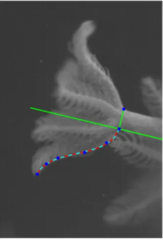
2.1 Sample image illustrating the methods used to track the kinematics over time. Blue dots correspond to the points tracked along the tentacle. Green lines correspond to the central axis of the base and a corresponding perpendicular line. The cyan curve corresponds to the dimensional polynomial fit and the red curve to the dimensionless polynomial fit (both are shown here to verify that the nondimensionalization is accurate). . . 14 2.2 Snapshots taken from a single polyp during tentacle contraction (A), expansion (B), and
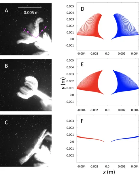
relaxation before the subsequent contraction (C). Position of a tentacle over time was tracked (in five different polyps for five different pulses), and the motion was fit with time varying polynomials and then averaged to describe the contraction (D), expansion (E), and relaxation (F). Red lines correspond to the leftmost tentacle at different instances in time, and the blue lines correspond to the rightmost tentacle. The base of the polyp is not shown and is assumed to be fixed. . . 15 2.3 Pulsing frequency vs. tentacle length for 15 corals in the field (Red Sea, Eilat, Israel)
and 15 cultured corals in the lab. The low R2 value does not support any significant relationship between pulsing frequency and size. . . 19 2.4 Velocity vector fields from PIV (A) and from a simulated polyp (B) combined with
a pressure colormap (B only) during one pulsing cycle. Snapshots are taken at 33% (i), 66% (ii), and 100% (iii) of the contraction and at 33% (iv), 66% (v), and 100% (vi) of the expansion. Vectors show the magnitude and direction of flow. The arrows correspond to the direction of flow, and the length and colors of the arrows correspond to the magnitude of the velocity. This simulated velocity field was taken from the 10th pulse of the simulation on a 2D slice through the central axis of the polyp. Note that the dynamic viscosity of the fluid was altered to match this particular real polyp (Ref ≈20). 21
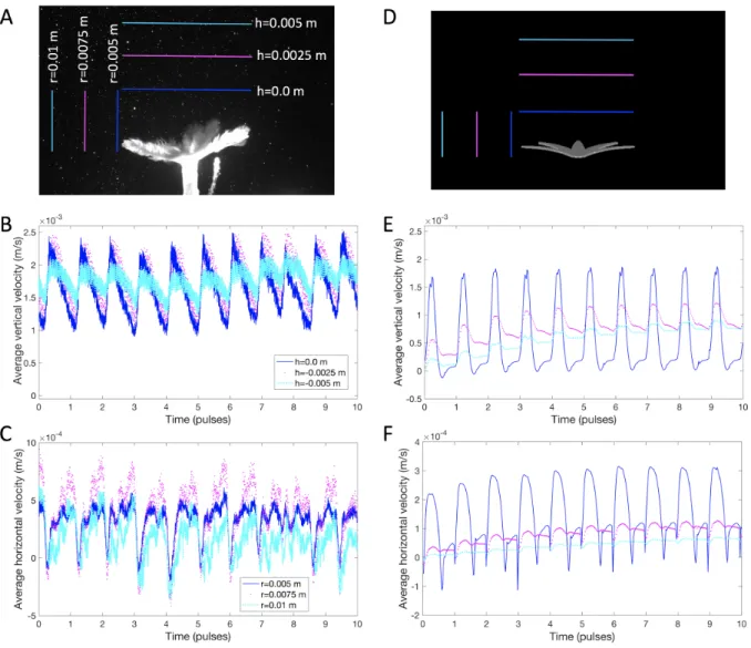
2.6 Comparison of flow velocities spatially averaged along a line in the x, y−plane in a real (A-C) and a numerically simulated (D-F) polyp over 10 pulsing cycles. Since the model is based on an average polyp, the dynamic viscosity of the fluid in the simulation was reduced to match the Ref of this particular polyp (Ref ≈ 20). A and D show the
horizontal positions over which the vertical flow away from the polyps was averaged at the top of the tentacles at the end of contraction (blue line) and at positions that are about one half (magenta) and about a full (cyan) tentacle length away. The vertical lines show the radial positions over which the horizontal component of the flow was averaged. These positions are at the tip of the tentacle when it is fully relaxed (blue) and at positions that are about one half (magenta) and about a full (cyan) tentacle length to the left. B and E show the vertical velocity averaged along the horizontal lines at the same three positions for the live polyp (B) and the simulation (E). C and F show the horizontal velocity averaged along the three vertical lines for the live (C) and simulated (F) polyp. 24 2.7 Contour plots of the finite-time Lyapunov exponent (FTLE) on a logarithmic scale
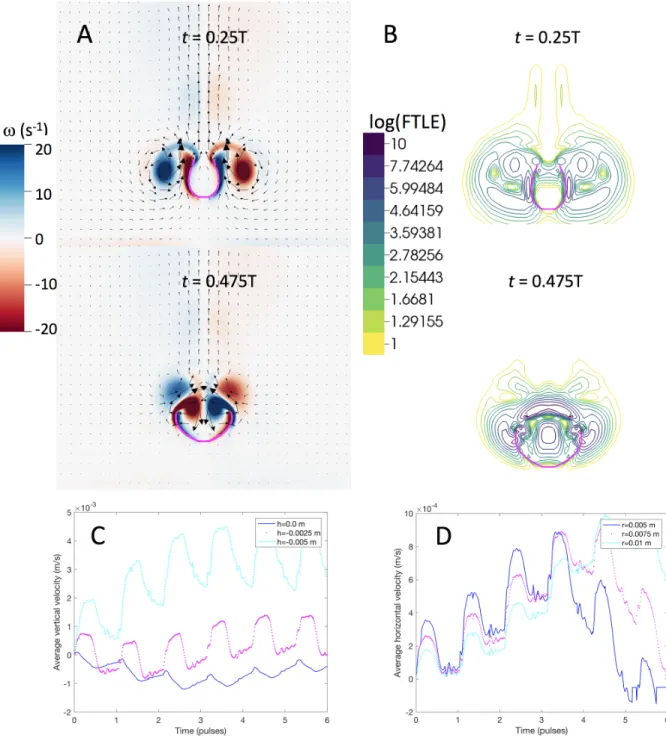
showing the instantaneous Lagrangian coherent structures (LCSs) during one pulsing cycle in a simulated polyp. Large FTLE regions divide areas of mixing. These are evident around the tentacles since the solid boundary divides the flow field. In addition, the slow flow between the tentacles is separated from the upward jet during expansion (note the blue-purple region above the top of the polyp). . . 26 2.8 Data from the 2D numerical simulation. (A) Snapshots of the vorticity and velocity field
during contraction and expansion. (B) Log(FTLE) of the instantaneous velocity vector field during contraction and expansion. (C) Vertical velocity averaged along three lines positioned 0, 0.0025, and 0.005 m above the tip of the tentacles at the end of contraction. (D) Horizontal (radial) velocity averaged along three lines positioned 0.005, 0.0075, and 0.01 m from the central axis of the polyp. Note that positive flow is towards the polyp. . 27 2.9 The z-component of vorticity and the velocity vector field taken on a 2D plane through
the central axis of the coral at Ref = 0.5, which corresponds to a smaller scale than
would be observed in nature. The colormap shows the value ofωz, the arrows point in
the direction of flow, and the length of the vectors correspond to the magnitude of the flow. Snapshots are taken during the fourth pulse at times that are 5%, 15%, 25%, 35%, 45%, 55%, 65%, and 75% through the cycle, such that the first three frames show the contraction phase, the next four frames show the expansion phase, and the last frame shows the polyp at rest. . . 30 2.10 The z-component of vorticity and the velocity vector field taken on a 2D plane through
the central axis of the coral atRef = 10, which corresponds to a typical Reynolds number
for a coral polyp in the field. The colormap shows the value of ωz, the arrows point in
the direction of flow, and the length of the vectors correspond to the magnitude of the flow. Snapshots are taken during the fourth pulse at times that are 5%, 15%, 25%, 35%, 45%, 55%, 65%, and 75% through the cycle, such that the first three frames show the contraction phase, the next four frames show the expansion phase, and the last frame shows the polyp at rest. . . 31 2.11 The z-component of vorticity and the velocity vector field taken on a 2D plane through
the central axis of the coral at Ref = 80, which corresponds to a much larger and faster
pulsing polyp than observed in nature. The colormap shows the value of ωz, the arrows
point in the direction of flow, and the length of the vectors correspond to the magnitude of the flow. Snapshots are taken during the fourth pulse at times that are 5%, 15%, 25%, 35%, 45%, 55%, 65%, and 75% through the cycle, such that the first three frames show the contraction phase, the next four frames show the expansion phase, and the last frame shows the polyp at rest. . . 32 2.12 The spatially averaged vertical flow above the polyp (top panel) and the spatially averaged
2.13 Temporally and spatially averaged vertical flow above the polyp (A), horizontal flow in the x−direction towards the polyp (B), and velocity magnitude between the tentacles (C) for varying values ofRef. Note that the velocities are nondimensionalized by the
tentacle length and pulse duration. . . 35 2.14 Contour plots of the finite-time Lyapunov exponents illustrating the instantaneous
Lagrangian coherent structures (LCSs) during a single polyp’s pulsing cycle for (A) Ref = 0.5, (B)Ref = 20and (C) Ref = 80, using a logarithmic scale. The LCSs were
calculated for the fourth pulse cycle using the entire 3D flow field but plotted on a 2D slice through the sagittal plane of the polyp. . . 36
3.1 Overview of the time bins that can be observed for a group of four polyps. Black cells correspond to pulse events (1) while white cells denote the absence of pulse event (0). . 43 3.2 Schematic diagram of the data collection. Raw video data were used in four different
ways for our analyses: 1) color videos were converted to black and white; 2) pulse timings of individual polyps were manually tracked and parameterized; 3) artificial colonies were generated by permutating data from polyps in different colonies; 4) artificial colonies were generated in which one, two, or three polyps would "lead" the other polyps (the lagging polyps were duplicates of the leading polyps but with an added lag in pulse timing). 45 3.3 Three representative extracts from the discretized data showing repetitive pulsing patterns.
Black cells correspond to pulse events while white cells denote the absence of pulse events. Time is given in seconds in time bins of 500 ms. . . 49 3.4 Examples of observed pulse patterns. Pulse patterns consist of loops of three combinations
as described in Figure 3.1. In a pattern, each polyps pulses once. . . 50 3.5 Extracts from the discretized data, the random model of collective pulsing, and the
Markov chain model of collective pulsing. Black cells correspond to pulse events while white cells denote the absence of pulse events. Time is given in seconds, time bins are 500 ms. Contrary to the live coral data, the random and Markov chain models fail to reproduce any observable pulse patterns. . . 51 3.6 Simulation results for the coupled phase oscillators model for varying coupling strengths
and polyps with Ki = 2 for all polyps. A coupling strength = 0 is equivalent to
completely uncoupled oscillators. Note that the time shown here start at 0. . . 52 3.7 Simulation results for the coupled phase oscillators model for varying coupling strengths
and polyps with differentKi around a value of 2. A coupling strength= 0is equivalent
to completely uncoupled oscillators. . . 53 3.8 (a) A sample in time of the pixel arrays sent to ISOMAP created from a sample of a
colony of six individuals. fi is the relative phase of each polyp as defined by equation
3.9 Total transfer entropy analysis for (A) real coral data, and (B) artificial data with similar sparsity but known interactions between polyps (I show here data for scenario 3 which is the least likely to show a significant outcome). In both cases, I first computed the mean total transfer entropy from all possible pairs of polyps within a given colony (14 colonies in total; time window of 20 frames; black dots). I then calculated the mean total transfer entropy for 1,000 surrogate datasets constructed from the original polyps but randomly paired between colonies in order to form groups of independent, non-interacting polyps. The extremities of the dashed lines represent the 2.5 and 97.5 percentiles of the surrogate distribution. If a dot falls within the range of the associated dashed line, it means that the average total transfer entropy for this colony does not significantly differ from an artificial colony made up of independent polyps. . . 55
4.1 Diagram of the three-dimensional coral polyp created in AutoDesk Fusion 360. . . 61 4.2 Position of the tentacles over time. Note that β is set toβm= 0.2during full contraction
and βo = 4.0during full expansion. . . 63
4.3 Instantaneous snapshots taken during the sixth pulsing cycle for a single polyp. The times shown are at 0, 1/8, 1/4, 3/8, 1/2, 5/8, 3/4, and 7/8 of the stroke cycle. The arrows point in the direction of flow and the colormap shows the out of plane vorticity. . 65 4.4 Spatially averaged vertical flow above a single coral polyp as a function of time over six
pulses. . . 66 4.5 Spatially averaged horizontal flow to the left of a single coral polyp as a function of
time over six pulses. Note that by averaging in this space and in this frame of reference, positive flow is towards the polyp. . . 67 4.6 Instantaneous snapshots taken during the sixth pulsing cycle for a pair of polyps pulsing
in phase. The distance between the polyps is 0.015 m. The times shown are at 0, 1/8, 1/4, 3/8, 1/2, 5/8, 3/4, and 7/8 of the stroke cycle. The arrows point in the direction of flow and the colormap shows the out of plane vorticity. . . 68 4.7 Instantaneous snapshots taken during the sixth pulsing cycle for two polyps pulsing 100%
out of phase. The distance between the polyps is 0.015 m. The times shown are at 0, 1/8, 1/4, 3/8, 1/2, 5/8, 3/4, and 7/8 of the stroke. The arrows point in the direction of flow and the colormap shows the out of plane vorticity. . . 69 4.8 Spatially averaged flows as a function of time for six pulse cycles. The phase difference
was varied from 0 toπ radians for a set distance of 0.015 m. (A) Vertical flow averaged above the left polyp; (B) vertical flow averaged over the right polyp; (C) horizontal flow averaged to the left of the left polyp. . . 71 4.9 Spatially and temporally averaged flows during the sixth pulsing cycle as a function of the
phase difference for a set distance of 0.015 m. (A) Vertical flow averaged above the left polyp; (B) vertical flow averaged over the right polyp; and (C) horizontal flow averaged to the left of the left polyp. The red lines correspond to the average flow for the single polyp. . . 72 4.10 Spatially averaged flows as a function of time for six pulse cycles. The distance between
polyps was varied from 0 to 0.028 m for a set phase difference ofπ/4. (A) Vertical flow averaged above the left polyp; (B) horizontal flow averaged to the left of the left polyp. The red lines correspond to the average flow for the single polyp. . . 74 4.11 Spatially and temporally averaged flows during the sixth pulsing cycle as a function of
LIST OF TABLES
2.1 Summary of experimental data measured from five polyps. . . 16 2.2 Numerical and physical parameters used in the immersed boundary simulations. . . 18
3.1 Number of video recordings and tracked polyps for each colony for the continuous-time approach. . . 41 3.2 Overview of the sub-hypotheses tested with the discrete-time approach. . . 56
4.1 Numerical parameters used in the three-dimensional simulations. . . 62 4.2 Overview of the peak magnitudes of the averaged flow velocities for the different polyp
CHAPTER 1
GENERAL INTRODUCTION
The present dissertation is the product of an interdisciplinary doctoral research project combining different aspects of biology and mathematics. This general introduction is intended to give the reader the necessary background information so that (s)he can come to a deeper understanding and appreciation of this body of research and can form his or her own judgement about its quality. The topics covered in this general introduction include the fluid dynamics of benthic organisms, basic concepts of collective behavior, and general information about pulsing corals, the organisms at the center of this research. Lastly, a short overview of the subsequent chapters provides a brief summary of the content of this dissertation.
1.1 Fluid dynamics of benthic organisms
The benthos is populated with fascinating organisms, many of which are invertebrates (worms, molluscs, arthropods, sponges, corals...). How these organisms experience their physical environment is very different from how we experience it, and studying them requires us to take these differences into account when we formulate hypotheses and design experiments. In this section, I will cover a few concepts relevant to the fluid dynamics of benthic organisms that will enable us to detach ourselves from our human perspective of benthic life and gain a more objective understanding of the behaviors and ecology of benthic organisms.
1.1.1 Reynolds and Péclet: two numbers to live by
One of the most objective ways to describe any environment is by using dimensionless numbers or assigning values to physical parameters so that we can quantitatively compare different environments to one another. For benthic environments, two numbers are relevant and used throughout the literature: the Reynolds number, Re, and the Péclet number, P e, both named after eminent physicists.
and is defined as
Re= ρLU
µ (1.1)
where ρ is the fluid density in kg/m3, L is a characteristic length (usually the greatest length of an object in the direction of the fluid flow [4, 5]) in m,U is the free-stream flow velocity in m/s, and µis the fluid’s dynamic viscosity in Pa/s or kg/m/s. When Re= 1inertial and viscous forces are equal, whenRe >1 inertial forces dominate, and whenRe <1 viscous forces prevail.
As can be seen in equation 1.1, theRe depends, in part, on the size of the organism considered. For example, two animals, a large whale and a tuna, swimming in the same fluid and at the same speed of 10 m/s, will experience the fluid differently; to the whale (Re= 3×10⁸), inertial forces will play a relatively more important role than to the tuna (Re= 3×10⁷). A bacterium swimming in the same seawater, albeit at a much slower speed of 0.01 mm/s, will experience the fluid as being primarily dominated by viscous forces (Re= 1×10⁻⁴). MoreRe values for different organisms can be found in Table 5.1 in [4]). For a human swimmer, the Reynolds number has been estimated to be Re= 4.5×10⁶ [6], i.e., one order of magnitude lower than for a tuna but ten orders of magnitude higher than for a bacterium.
Thus far, we computed the Reynolds number based on the environmental fluid flow velocity U and the sizel of the organism or object under consideration. The Reynolds number can however be defined at different scales such that the environmental Reexperienced by an organism and the localRef produced for example by the organism’s motion are considered to be different. In this
dissertation,Rewill be used for the environmental Reynolds number andRef will be used to describe
the Reynolds number derived from an organism’s movements, and in particular a pulsing coral polyp, and defined as
Ref =
ρL2f
µ (1.2)
where Lis the length of the appendage being moved (e.g., a tentacle) and f is the frequency with which it is moved.
The Péclet number describes the relative importance of advection over diffusion for a given substance and is defined as
P e= LU
where Land U are the characteristic length in m and the free-stream speed in m/s, respectively, and D is the diffusion coefficient of the given substance in m2/s [5]. Like the Reynolds number, the Péclet number is dimensionless. An organism operating at high P e can rely on advection (by swimming, pulsing, paddling, beating its cilia...) to influence mass transfer of nutrients and gases since the advection rate is larger than the diffusion rate for the mass under consideration. Conversely, a lowP e indicates that diffusion prevails and that spending energy is less effective in gaining access to more nutrients or getting rid of waste products [5].
1.1.2 Life in the boundary layer: the importance of size and behavioral strategies Beside issues related to inertial and viscous forces and advection and diffusion rates, benthic organisms also must cope with the phenomenon of the boundary layer resulting from the so-called no-slip condition. The no-slip condition states that, at a solid-fluid interface (i.e. the bottom of the sea), the fluid velocity equals the surface velocity, which is 0 [7]. In other words, the water velocity at the bottom is 0. In a laminar flow regime, the region of fluid between the bottom, where the no-slip condition applies, and the distance from this surface where the flow velocity reaches u= 0.99U, is called the boundary layer (Figure 1.1).
Depending on the environmental Re, boundary layers can be laminar, like in Figure 1.1, or turbulent. There tends to be much less mass transport in thez−direction in a laminar boundary layer, meaning stratified regions may develop in which mixing is low and nutrient depletion and/or waste accumulation occur [4]. This can become a problem for small organisms completely or in large part contained in this kind of boundary layer, as they may have difficulty gathering nutrients from their environment or getting rid of waste products. Two main strategies exist to avoid this problem: size increase or behavioral adaptations. Organisms that increase in size may extend (partly) out of the boundary layer, ensuring that at least part of their surface be exposed to regions of high mixing. Behavioral adaptations to life in the boundary layer include the generation of jets, the use of cilia or flagella to create local flows, or any other behavior resulting in increased fluid mixing and thus local reduction in boundary layer thickness.
1.2 Collective animal behavior
Figure 1.1: Schematic diagram of a laminar boundary layer above a no-slip surface. Ux is the flow
velocity in thex−direction,U is the free-stream flow velocity magnitude,z is the height above the bottom, and δ is the thickness of the boundary layer.
diverse disciplines such as biology, robotics, and social sciences. In animals, most collective behavior studies focus on eusocial insects such as ants or bees, or group-forming animals like birds, fishes, and humans [9]. Research on the collective behavior of non-insect invertebrates is limited, especially for marine invertebrates.
radius of the alignment zone, simulated groups display swarming behavior, move as a torus, or all members move parallel in the same direction, behaviors typical of fish schools. This example is just one of many models in which collective behavior becomes self-organized when individuals all follow the same, relatively simple behavioral rules. One less studied problem is coordination of collective behavior in groups of individuals that are physically connected to each other. In this thesis, I address this issue for the case of polyps in a coral colony.
For the purpose of clarity and consistency throughout this thesis, I define here a few terms that are related but not synonymous. First, collective behavior is a specific behavior or set of behaviors performed at the same time by members of a group. Second, coordinated or self-organized behavior encompasses all collective behavior in which a pattern can be quantitatively described; this pattern can be defined in time and/or space. It is important to note that all coordinated behavior, by definition, requires at least two individuals (so one individual can coordinate its behavior with that of the other individual) and is thus also considered to be collective behavior. The opposite is not always true: collective behavior is not necessarily coordinated [14]. Third, information transfer is the exchange of information between individuals about their current state or behavior. In groups, coordinated behavior can emerge in the absence of information transfer and information transfer can take place without it leading to coordinated (or even uncoordinated) collective behavior. For example, a group of kitchen timers all set to go off at the same time interval will display coordinated behavior but no information transfer is taking place between the timers. Conversely, a group of friends can exchange information about an upcoming party without all members of the group arriving at the same time or even attending the party. When studying collective behavior, it is important to keep these concepts in mind.
1.3 Study system: xeniid corals
1.3.1 Taxonomy, habitus, and geographic distribution
the Octocorallia is characterized by polyps bearing eight hollow tentacles, each fringed by one or several rows of pinnules [15], giving the polyps in this subclass a feathery aspect. Soft corals further belong to the order Alcyonacea, which also includes sea fans. Finally, the Xeniidae is one of about 30 families within the order Alcyonacea; the common name for this family of soft corals is "pulse corals" [16].
Xeniid corals thus form a family of soft corals known for the peculiar pulsing behavior noted by Lamarck [17] over 200 years ago and observed in several genera belonging to this group, such as Xenia spp. and Heteroxenia spp. Xeniids form colonies (Figure 1.2) up to 60 cm across [18] composed of tens to hundreds of polyps. Colonies consist of a common body or syndete and polyps with long stalks and flower-like heads or anthocodiae [19, 15, 16].
Figure 1.2: A colony of xeniid coral (probably Heteroxenia sp.) found off the dock of the Inter-University Institute (IUI) in Eilat, Israel.
in this dissertation I only identify the corals studied to the genus level.
Xeniids, and in particular Heteroxenia spp. and Xenia spp., are common in most tropical waters. Their geographical range extends from the east coast of Africa to Palau, and from Japan in the north to the Great Barrier Reef in the south [15]. They are common in the Red Sea, where I performed my fieldwork. Both genera are also known to be pioneering species on coral reefs, being among the first colonizers in new sites [16]; they can sometimes become invasive and encroach on other (hard) coral species.
1.3.2 Polyp anatomy and pulsing behavior
Very few studies of the polyp anatomy of xeniid corals are available and the diagrams of the histology as well as the written descriptions are limited. Gohar and Roushdy [3] distinguish two categories of the nervous system in Heteroxenia fuscescens: the sensory cells, found in both the ectodermal and endodermal layers, and the nerve plexus, composed of cells and fibrils that originated from the ectoderm. The nerve plexus is of interest here since it is involved in the pulsing behavior. In the polyps, the nerve plexus is further classified as an ordinary diffuse nerve net (the typical cnidarian nerve net also found in jellyfish) and the peristomial nerve net (Figure 1.3; [3]). The ordinary diffuse nerve net extends through the common body of the colony and the stalk of each polyp, linking them all to one another. The peristomial nerve net is found in each individual polyp head and plays a role in coordinating the eight tentacles of each polyp. Behavioral experiments show there is a separation between these two neural nets; when an individual polyp is stimulated, its tentacles will contract but this behavior will not spread to other neighboring polyps; on the other hand, if the syndete is stimulated, all polyps contract [19].
In their histological study, Gohar and Roushdy [3] describe the muscle fibers as similar to (in)vertebrate smooth muscle ("unstriped muscle fibres of higher animals"). They distinguish a concentric layer of muscle fibers around the mouth and longitudinal muscle fibers extend into the tentacles, but it is unclear where the former end and the latter begin. In their description of the oral disc muscle fibers, they add that the concentric muscle fibers are "continued peripherally and slightly upwards on the bases of the tentacles." They observe longitudinal muscle fibers on both the oral and aboral sides of the tentacles, so that both the opening and closing motions of the polyp are due to active muscle contraction [3].
Figure 1.3: Schematic drawing showing the neuromuscular anatomy of a Heteroxenia fuscescens polyp. Each polyp has two nerve nets: the peristomial nerve net (a) and the diffuse nerve net (b and c). The concentric muscle fibers around the oral disc are highlighted in red, the longitudinal muscle fibers going into the tentacles are highlighted in blue. The original figure and accompanying text do not detail how far up the tentacles the nerve nets can be found, where the muscles from the oral disc end and the muscles from the tentacles originate, or how the nerves and muscles interact (adapted from [3]).
1.3.3 Recent research on the pulsing behavior of xeniid corals
Few behavioral studies of corals exist and are often limited to reproductive behavior [27] and larval settlement [28]. The unique pulsing behavior displayed by xeniids was investigated by Gohar and his colleagues in the late 1950s [3, 19] and, more recently, by my collaborators at the Inter-University Institute (IUI) in Eilat [29]. Their study shows that the pulsing behavior is continuous except for short periods of rest of 15-30 min, usually around dusk. During pulsing, both the photosynthetic and the respiration rates increase by factors of two and seven, respectively. The increased photosynthetic rate is not so much due to an enhanced inflow of nutrients or CO2 but rather to an increase in the efflux of oxygen from the coral tissue [30, 29, 31]. At night, the pulsing is thought to reduce hypoxic stress and avoid refiltration of nutrient-depleted water. From a hydrodynamic perspective, the pulsing behavior changes the flow field above the coral colony, causing a stronger upward flow when the polyps are active. Simulations involving the release of hypothetical neutral density particles above a coral colony showed that the proportion of refiltered particles drops drastically from 50% of particles (non-pulsing colony) to 20% (pulsing colony).
Other recent research on xeniid corals mainly focus on species determination and identification [22, 23, 21], genetic diversity [32], coral response to acute exposure to chemicals [33], and metabolic activity [34].
Thus, additional research is needed, given the sparse attention to xeniid pulsing behavior and xeniid corals in general.
1.4 Research philosophy
For my dissertation research, I have employed an interdisciplinary approach involving a mix of complementary methods including experiments, computational simulations, and fieldwork. My experience is that, by tapping into different fields of science and expertises, we can gain insights into problems that did not yield to unilateral approaches. Although I spent a fair amount of time (approximately six weeks total between 2015 and 2017) in the field, most of the material presented
in this thesis will be of experimental and computational nature.
1.5 Thesis overview
observational data, I qualitatively and quantitatively describe the pulse kinematics and characteristic flow patterns of pulsing corals in quiescent flow and provide a range of Ref measured for corals in
a lab setting without background flow and for corals in the field. This chapter represents the first comprehensive and quantitative description of the pulsing behavior of soft corals. The second half of this chapter is dedicated to the design and testing of a 3D computational model to simulate pulsing polyps using the immersed boundary method (IBM). After validating the model, I compare the flow fields generated by the same polyp with the same kinematics at different environmentalRef. This
in-depth study of the flow fields generated by a pulsing polyp uncover a novel mechanism to mix fluid efficiently at intermediate Ref.
In the second chapter, I focus on the aspects of collective behavior in xeniid corals. From informal observations in the field and the lab, the collective pulsing behavior appears, at least locally, coordinated (small neighborhoods in which polyps seem to coordinate their behavior can be seen in a colony). Computer vision algorithms and information-theoretic tools are used to mine video data and uncover potential signs of coordinated behavior or information transfer between polyps. The results do not support the existence of such behavior, however, and models involving (coupled) phase oscillators reiterate that it is possible to observe pulsing patterns in polyp groups even in the absence of coordination.
Finally, in the third chapter, I integrate information from the first two chapters to investigate the effects of collective pulsing behavior on local fluid flows. First, I compare the flow fields of a single polyp with those of polyp pairs to determine if there are any benefits to pulsing in a group (lower energetic cost per individual polyp, greater mass transfer...). Second, I examine the effect of pulse timing on the produced flow fields by varying the phase difference between two pulsing polyps (ranging from two polyps pulsing in-phase to two polyps pulsing completely out-of-phase). Third, I
increase the distance between polyps to measure its effect on the flow fields.
CHAPTER 2
A NOVEL MECHANISM OF MIXING BY PULSING CORALS
2.1 Introduction
For sessile organisms like corals, having the ability to enhance nutrient and gas exchange can result in increased fitness and survival [30, 31]. As described in the general introduction, mass transfer is influenced by the presence of boundary layer and characteristics of the fluid environment, which can be determined by the Péclet and Reynolds numbers. Mass exchange in the benthic layer is a multiscale process with different constraints depending on the scale under consideration. At lowRe andP e, viscous forces and diffusion prevail but these limitations can be offset by increasing the local Reynolds number through motion (consideringRef instead of Re). Active flow generation
among corals is mostly limited to the microscale: many coral species possess epidermal cilia whose beating can break the diffusive boundary layer near the coral tissue and increase the mass transfer of oxygen from the tissue to the surrounding water [35]. The effect of the cilia beating, however, decreases rapidly with increasing intensity of the ambient flow (increasingRe from background flow). Xeniid corals, with their peculiar pulsing behavior, display a behavioral adaptation to increase mass transfer at the tentacle and polyp scale. The collective pulsing behavior also affects the flow velocities and thus the Ref at the colony level [29]. While this kind of flow-generating behavior
is relatively common among macroscopic marine animals, with examples ranging from the active contractions of jellyfish bells for swimming [36, 37, 38] and feeding [39, 40], fast contraction of the mantle for jet propulsion in squid, octopus and other cephalopods [41, 42], and fast closing of the shells in scallops [43], it is usually observed at scales where inertial forces in the fluid dominate over viscous forces, more specifically when the Reynolds number of the system (Ref) is on the order of
100 or more. In general, corals cannot achieve such values of Ref; mass transport in most corals is
governed by larger-scale processes, like local water flows, that increase the environmental Re[44, 45]. Pulsing corals operate at a much lower Ref regime than the only other benthic cnidarian known
upside-down jellyfish host zooxanthellae in their tissues [46, 47]. Unlike soft corals that generate exchange currents with their tentacles, upside-down jellyfish create flow by actively contracting and relaxing their gelatinous bell and pushing flow through an array of elaborate oral arms. The biologically relevant Ref for upside-down jellyfish pulsing in the benthic layer ranges from about
100 to approximately 450 for an adult [48]. As such they operate completely within the inertial range (Ref >>1) where reciprocal motions are effective. On the other hand, pulsing corals produce
exchange jets at scales where viscous forces in the fluid become significant (Ref ≈10) and the use
of reciprocal motions for propulsion and the generation of feeding currents becomes less efficient [49, 50, 51, 52]. It is therefore unclear how xeniid corals use their pulsing motion to generate efficient mixing. Accordingly, the movements of pulsing soft corals generate interesting fluid dynamics that push the limits of mixing jets into the viscous regime, potentially inspiring the design of efficient small-scale mixers.
The goal of this chapter is to gain understanding of the kinematics and fluid flows generated by a single pulsing polyp using high-speed video and particle image velocimetry (PIV). Since PIV measurements of the flow between the tentacles are difficult to obtain due to limited optical access, intensive three-dimensional simulations using the immersed boundary method (IBM) were also conducted to model these flows. The empirical results were used to validate the simulations. Beside visualizing flow patterns between the tentacles, the model was also used to quantify the fluid dynamics of a pulsing polyp over a range ofRef, both above and below the biologically relevant
range. Alternatively, it could be used to explore the effects of different pulsing kinematics on the generated flow patterns.
2.2 Materials and Methods 2.2.1 Data collection
absence of flow (quiescent background).
Particle Image Velocimetry (PIV) PIV data was collected from a colony consisting of one polyp. The camera was focused on the polyp to resolve the flow through its central axis. PIV videos were taken along the vertical (stem) axis of the polyp, at its sagittal plane. I used neutrally buoyant, hollow glass beads of 10 micrometer diameter and a Photron SA3 120K camera with a 105 mm NIKKOR lens. The videos were recorded at 125 fps. The camera was operated using PFV software [53]. The laser was a continuous Genesis MX 523 -8000 with a custom-built optical system. The wavelength of the laser was 532 nm, and it was operated at approximately two watts.
No pre-processing of the images was performed. PIV calculations were done on sequential images using the freely accessible OpenPIV package in Python [54] with interrogation and search window sizes of32×32 pixels and an overlap of 16 pixels. A white threshold was set to automatically mask the polyp and its reflections from the laser. Post-processing of the velocity vector fields involved interpolation to fill in rejected vectors. The velocity vector fields were plotted using custom-written Python code using the instantaneous velocity fields for each frame of the video.
nondimensionalx- and y-positions as functions of the nondimensional arclength (Figure 2.1; red curve). A quick calculation of the Péclet number for oxygen, based on the bulk flow around the polyp, with L= 0.00407m, U = 0.0025 m/s, andD= 1.9569×10⁻⁹ m2/s results in P e= 5199, meaning that oxygen transport at the scale of the polyp is dominated by advection. Increasing local water motion through pulsing is thus expected to enhance oxygen transfer at this scale.
Figure 2.1: Sample image illustrating the methods used to track the kinematics over time. Blue dots correspond to the points tracked along the tentacle. Green lines correspond to the central axis of the base and a corresponding perpendicular line. The cyan curve corresponds to the dimensional polynomial fit and the red curve to the dimensionless polynomial fit (both are shown here to verify that the nondimensionalization is accurate).
Figure 2.2: Snapshots taken from a single polyp during tentacle contraction (A), expansion (B), and relaxation before the subsequent contraction (C). Position of a tentacle over time was tracked (in five different polyps for five different pulses), and the motion was fit with time varying polynomials and then averaged to describe the contraction (D), expansion (E), and relaxation (F). Red lines correspond to the leftmost tentacle at different instances in time, and the blue lines correspond to the rightmost tentacle. The base of the polyp is not shown and is assumed to be fixed.
Table 2.1: Summary of experimental data measured from five polyps.
Name Variable Units Value
Pulsing period T s 1.89±0.267
Duration of contraction Tc s 0.546±0.091
Duration of expansion Te s 0.706±0.033
Resting time Tr s 0.640±0.267
Tentacle length Lten m 0.00407±0.00029
Reynolds number Ref − 8.55±2.18
Fluid density ρ kg/m3 1.023×10³
Fluid dynamic viscosity µ kg/(ms) 1.08×10⁻³
2.2.2 Numerical simulations
The Immersed Boundary Method (IBM) The IBM [56, 57] was used to solve the fully coupled fluid-structure interaction problem of a pulsing soft coral in an incompressible, viscous fluid. This method has been successfully applied to a variety of problems in biological fluid dynamics in an intermediateRe regime (0.01< Re <1000), including cardiac blood flow and heart development [58, 59, 60, 61], flow past leaves [62], insect flight [63, 64], swimming [65, 66, 38], and even dating and relationships [67].
One of the main advantages of the IB method is that it is a straightforward way to handle the interactions between a fluid and an immersed structure with complex moving geometry. A Cartesian grid that is either uniform or uniform near the boundary can be used to solve the Navier-Stokes equations with a standard fluid solver. The immersed boundary (the coral polyp) is represented by a collection of Lagrangian markers that move independently from the Cartesian grid. The effect of the motion of the immersed boundary is transferred to the fluid grid through a simple-to-implement local stencil near each marker point and vice versa. I prescribed the preferred motion of the simulated polyp based on the tracking data I collected.
The numerical parameters used for the simulations are given in Table 2.2. The details of the IBM and the IBAMR can be found in Appendix 5.
Computational model The computational model of the coral consisted of eight tentacles and a base. The shape and size of the tentacles were determined from images of a single polyp. Given the low Re with respect to the diameter of a single pinnule on the tentacle, simulated tentacles were assumed to be solid plates. The width at the top of the tentacles was reduced to prevent overlap during the full contraction. The stem was not included in the simulations as it did not appreciably affect the flow. The kinematic data obtained from tracking polyp tentacles were used to prescribe the preferred position of the tentacles in the numerical simulations.
The computational domain was set to be a0.06×0.06×0.06m3with periodic boundary conditions in thex- andy-directions and no-slip boundary conditions in the z-direction. The polyp was placed in the bottom center of the computational domain. To build a computational polyp, I used a base to which I attached eight identical tentacles. The base of the tentacles was positioned 0.005 m above the bottom of the domain, approximately the length of the stem of a polyp. The average diameter of the base was determined by measuring and then averaging the distance between the bases of two oppositely arranged tentacles in each video frame. The average base diameter was 0.00106 m. Each tentacle was assumed to have the shape of an isosceles trapezoid with a basal width of 0.00108 m (the average width across all measured polyps). The apical width of each tentacle was set to be 1/5 of the basal width to prevent overlap of the tentacles during contraction. The distance from the center of the polyp base to the tip of each tentacle was approximately 0.0045 m when the polyp was fully extended and 0.0037 m when the polyp was fully contracted. The length of the tentacles was determined by averaging the lengths measured in each frame for each polyp used to track tentacle motion and then averaging the mean tentacle length of all five polyps. A summary of all numerical parameters is given in Table 2.2.
Table 2.2: Numerical and physical parameters used in the immersed boundary simulations.
Name Variable Units Value
Domain size D m 0.06
Spatial grid size dx m 5.86×10⁻⁵
Boundary grid size ds m 2.93×10⁻⁵
Total simulation time Ttot pulses 10
Time step size dt sec 1.22×10⁻⁴
Fluid density ρ kg/m3 1.0×10³
Fluid dynamic viscosity µ kg/(ms) 1.0×10⁻³
Target point stiffness ktarget kg∗m/s2 9.0×10⁻⁹
Tentacle length LT m 0.00407
Pulsing Period T sec 1.9
2.2.3 Varying the frequency-based Reynolds number
The frequency-based Reynolds numberRef was used to describe the flows produced by the polyp.
The characteristic lengthL was set to the tentacle length and the characteristic frequencyf was set to the polyp pulsation frequency given in Table 2.1.
To determine the biologically relevant range ofRef, videos of three coral colonies were acquired
in the Red Sea off the coast of Eilat, Israel, and of three colonies of cultured corals in the lab. In each video, five individual polyps were tracked to determine the average pulse period over 20 cycles. For each polyp, I also measured the length of one tentacle. I found no significant correlation between pulsing frequency and tentacle length (Figure 2.3). The averageRef was 19.64±7.28 with
a minimum of 8.74 and a maximum of 36.0. The average tentacle length was(6.13±0.10)×10−3 m and the average pulsing frequency was 0.53 ±0.043 Hz. For the numerical simulations with varying Ref, the frequency was set to that of a typical polyp with f = 1/1.9s−1. The dynamic viscosity of
water was varied to simulate a range of Ref with values above and below those typically experienced
by soft corals. The Ref values studied here is 0.5, 1, 5, 10, 20, 40, and 80.
2.2.4 Data analysis
Figure 2.3: Pulsing frequency vs. tentacle length for 15 corals in the field (Red Sea, Eilat, Israel) and 15 cultured corals in the lab. The low R2 value does not support any significant relationship between pulsing frequency and size.
the polyp and in the vertical direction above the polyp were computed from the experimental and computational data and the obtained flow fields were compared. For the PIV data and the base model, the vertical velocity in the upward jet was averaged along a line in the x, y−plane at the height of the tentacle tips during full contraction as well as at positions about one half and one full tentacle length above that tentacle tip height. The horizontal velocity towards the polyp was averaged at the tentacle tips during full expansion as well as at positions about one half and one full tentacle length to the left of that first position. For the simulations with varying Ref, the
x−component of the velocity (in the horizontal direction) was averaged within a box drawn from the tips of the tentacles during full expansion to one tentacle length to the left of that point (−0.009 m < X <−0.0045m). In thez−direction, the box was drawn along the diameter of the fully expanded polyp (−0.0045 m< Z <0.0045 m). In the vertical direction, the box was drawn from the polyp base to the top of the fully contracted tentacles (−0.01 m< Y <−0.0063 m).
for example in prey-predator interactions and locomotion [74, 75, 76]. Trajectories were computed using an instantaneous snapshot of the vector field and the FTLEs were computed on a regular1283
grid using a forward Dormand-Prince (Runge-Kutta) integrator with a relative tolerance of 0.001 and an absolute tolerance of 0.0001. The maximum advection time was limited to 0.1 s, and the maximum number of steps was set to 1000.
2.3 Results
2.3.1 Flow field generated by a single polyp
Figure 2.4A shows the velocity vector field generated by a real polyp at Ref = 20. Figure
2.4B shows its simulated counterpart atRef ≈20. For both polyps, the vector field represents the
direction (arrows) and magnitude (arrow length and color) of flow. I emphasize four characteristics of the flow:
1. A continuous jet away from the polyp. The direction of the jet is aligned with the polyp’s stem axis and is narrowly delimited (approximately the width of the closed polyp). Water is pulled in the horizontal (radial) direction towards the polyp and then ejected up and away from the tentacles. This flow pattern minimizes back flow, allowing for the sampling of new "fresh" fluid throughout the pulse cycle.
2. Starting and stopping vortices. The starting vortices are formed during contraction (i and ii) and rotate towards the outside of the polyp (counterclockwise for the left vortex, clockwise for the right vortex) whereas the stopping vortices are formed during expansion (v) and rotate in the opposite direction compared with the starting vortices.
3. A flow separation above the polyp during expansion (v). The flow well above the polyp continues to move in an upward jet while the flow directly above the polyp reverses, moves downward, and circulates over the tentacles.
Figure 2.5A shows the vorticity and streamlines within a two-dimensional slice cut through the sagittal plane of the real polyp at Ref = 20. The colormap corresponds to the value of the
vorticity with red representing counterclockwise flow and blue representing clockwise flow. Before contraction begins, a stopping vortex ring from the previous pulse cycle is visible above the open tentacles (vi) and rotating up and away from the polyp’s center. At the beginning of contraction, an oppositely spinning starting vortex ring is formed at the tips of the tentacles (i-ii). Towards the end of contraction and the beginning of expansion (iii-iv), the vortex ring moves to the outer surface of the tentacles and is advected up and away from the polyp’s central axis. The presence of this vortex ring enhances the upward jet since it rotates so that the fluid in the center of the ring is pushed up (iv-v). During expansion, an oppositely spinning stopping vortex is formed at the tips of the tentacles that drives mixing within the polyp (iv-vi).
2.3.2 Validating the computational model
Figure 2.6: Comparison of flow velocities spatially averaged along a line in thex, y−plane in a real (A-C) and a numerically simulated (D-F) polyp over 10 pulsing cycles. Since the model is based on an average polyp, the dynamic viscosity of the fluid in the simulation was reduced to match the Ref
of this particular polyp (Ref ≈20). A and D show the horizontal positions over which the vertical
2.3.3 Flow field analysis
Figure 2.7 shows contours of the log of the finite-time Lyapunov exponents (FTLE) which illustrate the instantaneous Lagrangian coherent structures (LCS). The contours are shown in a 2D slice through the central axis during one pulsing cycle for a simulated polyp using the averaged kinematics atRef = 20. Note that the LCS were calculated using the entire 3D flow field. Lagrangian
coherent structures identify regions of the flow that are attractive (small FTLE) or repelling (large FTLE) [72]. By revealing the regions of fluid that repel or are ‘separated’, one can understand which portions of the fluid are sampled by the organism and which portions pass by the animal without interacting. During contraction, radial flow is pulled towards the polyp but moves into the upward jet (t= 0.025T −0.325T). The large FTLE’s around the tentacles indicate that this flow does not mix with the fluid between the tentacles. The FTLE values above the polyp are small, indicating that the flow between the tentacles mixes with the upward jet. During expansion (t= 0.475T −0.625T), large FTLE values are observed above the polyp, which show that the region of fluid between the tentacles does not mix with the upward jet. This creates a slow-mixing region between the tentacles. Note that the 2D contour slice is taken along the tentacles. 3D visualization of the contours (not shown) reveals that flow does move between the tentacles and into the central region during expansion. This implies that new fluid is brought in during the tentacle expansion. Upon the next contraction, this fluid will be expelled upward into the jet and this cycle repeats during the next pulsation. When the polyp is at rest (t= 0.775T), the values of the FTLE are small and the fluid is slowly swept over the tentacles and into the upward jet.
2.3.4 Two-dimensional versus three-dimensional simulations
Figure 2.7: Contour plots of the finite-time Lyapunov exponent (FTLE) on a logarithmic scale showing the instantaneous Lagrangian coherent structures (LCSs) during one pulsing cycle in a simulated polyp. Large FTLE regions divide areas of mixing. These are evident around the tentacles since the solid boundary divides the flow field. In addition, the slow flow between the tentacles is separated from the upward jet during expansion (note the blue-purple region above the top of the polyp).
is more separated from the upward jet during contraction in 2D, and that there is less overall mixing between the tentacles during expansion in 2D.
Panels C and D in Figure 2.8 show the averaged vertical and horizontal flow, respectively, taken along lines that correspond to those used to characterize the three-dimensional simulations and experimental flow fields in Figure 2.6. During full contraction, average vertical flow at the tentacle tips (h = 0.0m) is predominately downward and into the area between the tentacles. This is in contrast to the positive flow observed in both the live polyp and the three-dimensional simulation. At 0.0025 m above the tentacle tips, the flow oscillates between positive and negative values, again in contrast to the live polyp and 3D simulations. At a full tentacle length above the polyp (h= 0.005
necessary to perform 3D simulations to accurately model pulsing polyps.
2.3.5 Varying the frequency-based Reynolds number
Once I validated the 3D model, I used it to study the effect of varying the Reynolds number on the observed flow field generated by the polyp. I performed simulations with0.5< Ref <80and
show snapshots of three cases in Figures 2.9, 2.10, and 2.11. The flow fields generated at these three differentRef are described below.
Regardless of Ref, the simulations generate a clear upwards jet during contraction and vorticity
at the tips of the tentacles. Oppositely spinning starting vortices are formed at the tips of each tentacle at the beginning of expansion (t= 0.35T). At higherRef, particularlyRef = 80, these
vortices separate from the tentacle tips and are advected upwards. Their motion helps to maintain a strong upward jet away from the polyp. At the lower Ref, (e.g. Ref = 0.5), these vortices
quickly dissipate and the flow above the polyp is reversed during expansion such that fluid is pulled downward between the tentacles. ForRef <1, the flow is nearly reversible; any fluid pushed away
from the polyp during contraction is pulled back during expansion. At intermediateRef (e.g. Ref
= 10), an upward jet is observed above the polyp during expansion, and fluid below this jet mixes between the tentacles. In both the Ref = 10and the Ref = 80cases, some flow is moving upward
during expansion (more in the case ofRef = 80). Near to the bottom of polyp, fluid is brought into
the polyp through the formation of vortices at the ends of the tentacles. During the resting phase (last frame), the fluid almost completely comes to rest in the lowerRef cases.
Although the strength of the upwards jet is greatest for Ref = 80, the flow magnitudes generated
between the tentacles by the stopping vortices (expansion) are greater for Ref = 0.5 andRef = 10.
There is strong mixing between the tentacles for Ref ≤30; this mixing decreases forRef >30. This
indicates that, near the biologically relevant Ref, the morphology and motion of the tentacles allow
for greater mixing close to the polyp itself.
To compare the relative strength of the upward jets across scales, the y−component of the velocity (in the vertical direction) was averaged within a box drawn above the simulated polyp. The height of the box extended from the tips of the tentacles during full contraction to one tentacle length above that point (-0.0063 m < Y <-0.0018 m). The width of the box was set equal to the diameter of the fully expanded polyp (-0.0045 m< X, Z <0.0045 m). Figure 2.12 shows the average vertical velocity over five pulses forRef =0.5, 1, 5, 10, 20, 40, and 80. Note that the velocities are
For each value of Ref, there is a peak average velocity in the upward jet corresponding to the
end of the polyp contraction. Moreover, the largest peak average velocity corresponds to the lowest Ref = 0.5 case, while the lowest peak corresponds to the highestRef = 80 case. This is partially
due to the fact that the flow velocity was averaged over a relatively large box. Additionally, the region of motion is larger at lower Ref due to the relatively large boundary layers (Ref was lowered
in the simulations by increasing only the dynamic viscosity). Immediately following contraction, as the polyp begins to expand, the average velocity drops for each Ref. There is significant back flow
(the average velocity becomes negative) for Ref <5. Around Ref ≥10 the average vertical flow
decreases during tentacle expansion but the net average flow remains positive (upwards). This is significant as the continuous upward jet allows new fluid to be brought to the polyp throughout the pulsing cycle.
The transition to continuous upward flow (no flow reversal) occurs at Ref = 10. For10≤Ref ≤ 30, the tentacle morphology allows for greater mixing near the polyp itself. These observations suggest that the polyp may be able to enhance its nutrient uptake or waste removal in this 10≤Ref ≤30
range. At Ref = 80 there is a continuous upward jet but little mixing near the polyp, meaning less
opportunity for the polyp to exchange nutrients and waste with its surrounding water. Wastes as well as nutrients would continuously be expelled away from the polyp, leaving less possibility for nutrient absorption. At Ref <10, there is more mixing near the polyp but the resulting flows are
unable to remove wastes away from the polyp (no continuous upward jet).
The vertical flow above the coral in Figure 2.13A is a temporal average of the fourth pulse. Figure 2.13B illustrates the temporally averaged horizontal flow of the fourth pulse. Panels A and B in Figure 2.13 highlight two flow phenomena that depend onRef. First, as Ref decreases, the
tentacles entrain a larger volume of fluid that is pulled towards the polyp and then upward into a vertical jet. This leads to a wider upward jet and thus larger spatially averaged velocities. Second, asRef decreases, the flow in the jet becomes increasingly reversible: up and away from the polyp
during contraction and back towards the polyp during expansion. Net volumetric flow is maximized for Ref between about 20 and 30. Reduction in net flow is observed for Ref ≈1 and lower because
the flow becomes progressively reversible. The net flow is reduced asRef increases above 30 because
Figure 2.9: Thez-component of vorticity and the velocity vector field taken on a 2D plane through the central axis of the coral at Ref = 0.5, which corresponds to a smaller scale than would be
observed in nature. The colormap shows the value of ωz, the arrows point in the direction of flow,
Figure 2.10: Thez-component of vorticity and the velocity vector field taken on a 2D plane through the central axis of the coral at Ref = 10, which corresponds to a typical Reynolds number for a
coral polyp in the field. The colormap shows the value of ωz, the arrows point in the direction of
Figure 2.11: Thez-component of vorticity and the velocity vector field taken on a 2D plane through the central axis of the coral atRef = 80, which corresponds to a much larger and faster pulsing
polyp than observed in nature. The colormap shows the value ofωz, the arrows point in the direction
Figure 2.12: The spatially averaged vertical flow above the polyp (top panel) and the spatially averaged horizontal flow towards the polyp (bottom panel) over time during five pulse cycles. Ref = 0.5, 1,5,10,20,40, and80are shown. Velocity is nondimensionalized and given as tentacle lengths per pulse.
This was performed in a volume defined by -0.001 m < X <0.001 m, -0.009 m < Y <-0.001 m, and -0.001 m < Z <0.001 m. The magnitude of flow generally decreases for increasing Ref, suggesting
that more of the fluid is directed into a narrow upward jet as the polyps grow larger. On the other hand, strong flow is generated between the tentacles at Ref below the biologically relevant range.
Figure 2.14 shows FTLE contours, illustrating the LCSs in our simulations for different values of Ref. Small values of the FTLE highlight regions where flow is attractive whereas small FTLE
values indicate areas in which the flow is repelling [72]. In the case of coral polyps, LCSs can be used to highlight regions of fluid that the polyps may sample or, alternatively, that may pass by without interacting with the organisms.
In the biologically relevant case (Figure 2.14B) and at higher Ref (Figure 2.14C), fluid is pulled
towards the polyp and pushed into the upward jet during the contraction phase (t= 0.073T and t = 0.17T). The FTLE values are small (attractive) between the tentacles during contraction, indicating that, in this area, the fluid is pushed upward and into the vertical jet. The large FTLE values near the tentacles show that fluid is repelled around the tentacles and the starting vortices. In other words, flow does not pass through the simulated tentacles but between them. These observations can only be made with 3D simulations as the space between tentacles needs to be visible. Comparison with the viscous-dominated case ofRef = 0.5(Figure 2.14A) shows a region of
larger FTLE values between the tentacles. This indicates that the fluid near the base of the polyp does not mix as well with the upward jet and is not fully expelled during contraction at lowerRef.
During expansion (t= 0.37T and t= 0.51T), large (repelling) FTLE values directly above the polyp and between the tentacles indicate a region of mixing that is separated from the upward jet in the biologically relevant case (Ref = 20). There also are larger FTLE values in the higher Ref case
(Figure 2.14C), but with a more complicated pattern between the tentacles indicating separated mixing regions. For the viscous-dominated case (Figure 2.14A), the FTLE values are low once the tentacles have partially expanded (t= 0.51T). This indicates that the upward jet and the mixing region between the tentacles are no longer separated, and indeed fluid is pulled from above the polyp and into the region between the tentacles (back flow). At thisRef, a new volume of fluid would not
Figure 2.13: Temporally and spatially averaged vertical flow above the polyp (A), horizontal flow in the x−direction towards the polyp (B), and velocity magnitude between the tentacles (C) for varying values ofRef. Note that the velocities are nondimensionalized by the tentacle length and
Figure 2.14: Contour plots of the finite-time Lyapunov exponents illustrating the instantaneous Lagrangian coherent structures (LCSs) during a single polyp’s pulsing cycle for (A) Ref = 0.5, (B)
Ref = 20 and (C) Ref = 80, using a logarithmic scale. The LCSs were calculated for the fourth
2.4 Discussion
Using quantitative PIV measurements and 3D numerical simulations, I have accurately resolved the flow near an individual pulsing coral polyp. The contraction, expansion, and relaxation kinematics generate a sustained jet away from the polyp and a slow region of mixing between the tentacles during expansion. This mixing volume is ejected into the vertical jet upon each contraction. The persistent vertical velocity advects oxygen-rich water away from the coral’s external envelope; however, this jet alone would not be sufficient without a mixing mechanism and a minimal retention time to allow for gases and nutrients to diffuse across the polyp tissue. Retention is needed to allow diffusion of oxygen from the tissue, enriched in oxygen by photosynthesis, to the surrounding water. The flow structure between the tentacles mixes the water that surrounds the tissue with new water that arrives radially to the internal space of each coral polyp. Without such a retention period and mixing, the efficiency of advection by the positive vertical jet might be reduced substantially. This hydrodynamic study serves as a strong indication that the coral has developed an efficient flow field to enhance oxygen removal and increase photosynthetic rates.
The only other sessile organism exhibiting similar behavior is the upside-down jellyfishCassiopea spp. which was reported to use pulsation to actively generate feeding currents [40, 51]. The basic flow structures observed here (upward jet and oppositely spinning starting and stopping vortex rings) are similar to those generated by the upside-down jellyfish. It is interesting to note that these flow patterns are generated in different ways and in different environments. In the case of the soft corals, eight long tentacles expand and contract to pull in fluid between them at relatively lowRef.
For upside-down jellyfish, a shallow bell contracts and expands, similarly generating starting and stopping vortex rings at much higher Ref, typically on the order of 100 or more. The upward jet is
continually pushed through an elaborate array of oral arms. Pulsing soft corals are often found in regions of relatively strong flow while upside-down jellyfish prefer slow-moving water or stagnant areas. It is interesting to consider how the differences in morphology and kinematics may be adapted to the differences in flow environment, boundary layer size, and scale.