Astronomy&Astrophysicsmanuscript no. taurus_binaries_alma cESO 2019 July 10, 2019
Observational constraints on dust disk sizes in tidally truncated
protoplanetary disks in multiple systems in the Taurus region
C.F. Manara
1,?, M. Tazzari
2, F. Long
3,4, G.J. Herczeg
3, G. Lodato
5, A.A. Rota
5, P. Cazzoletti
6, G. van der Plas
7,
P. Pinilla
8, G. Dipierro
9, S. Edwards
10, D. Harsono
11, D. Johnstone
12,13, Y. Liu
6,14, F. Menard
7, B. Nisini
15,
E. Ragusa
9,5, Y. Boehler
7, and S. Cabrit
16,71 European Southern Observatory, Karl-Schwarzschild-Strasse 2, 85748 Garching bei München, Germany e-mail:cmanara@eso.org
2 Institute of Astronomy, University of Cambridge, Madingley Road, CB3 0HA, Cambridge, UK 3 Kavli Institute for Astronomy and Astrophysics, Peking University, Beijing 100871, China 4 Department of Astronomy, School of Physics, Peking University, Beijing 100871, China 5 Dipartimento di Fisica, Universita Degli Studi di Milano, Via Celoria, 16, I-20133 Milano, Italy
6 Max-Planck-Institut für Extraterrestrische Physik, Giessenbachstrasse 1, 85748, Garching bei München, Germany 7 Univ. Grenoble Alpes, CNRS, IPAG, F-38000 Grenoble, France
8 Max-Planck-Institut für Astronomie, Königstuhl 17, 69117, Heidelberg, Germany 9 Department of Physics and Astronomy, University of Leicester, Leicester LE1 7RH, UK 10 Five College Astronomy Department, Smith College, Northampton, MA 01063, USA 11 Leiden Observatory, Leiden University, P.O. box 9513, 2300 RA Leiden, The Netherlands
12 NRC Herzberg Astronomy and Astrophysics, 5071 West Saanich Road, Victoria, BC, V9E 2E7, Canada 13 Department of Physics and Astronomy, University of Victoria, Victoria, BC, V8P 5C2, Canada
14 Purple Mountain Observatory, Chinese Academy of Sciences, 2 West Beijing Road, Nanjing 210008, China 15 INAF–Osservatorio Astronomico di Roma, via di Frascati 33, 00040 Monte Porzio Catone, Italy
16 Sorbonne Université, Observatoire de Paris, Université PSL, CNRS, LERMA, F-75014 Paris, France
Received May 27, 2019; accepted July 6, 2019
ABSTRACT
The impact of stellar multiplicity on the evolution of planet-forming disks is still the subject of debate. Here we present and analyze disk structures around 10 multiple stellar systems that were included in an unbiased, high spatial resolution survey of 32 protoplanetary disks in the Taurus star-forming region with ALMA. At the unprecedented spatial resolution of∼0.1200
we detect and spatially resolve the disks around all primary stars, as well as those around eight secondary and one tertiary stars. The dust radii of disks around multiple stellar systems are smaller than those around single stars in the same stellar mass range and in the same region. The disks in multiple stellar systems have also a steeper decay of the mm-continuum emission at the outer radius than disks around single stars, suggestive of the impact of tidal truncation on the shape of the disks in multiple systems. However, the observed ratio between the dust disk radii and the observed separation of the stars in the multiple systems is consistent with analytic predictions of the effect of tidal truncation only if the eccentricities of the binaries are rather high (typically>0.5), or if the observed dust radii are a factor of two smaller than the gas radii, as is typical for isolated systems. Similar high resolution studies targeting the gaseous emission from disks in multiple stellar systems are required to resolve this question.
Key words. Protoplanetary disks - binaries: visual - binaries: general - Stars: formation - Stars: variables: T Tauri, Herbig Ae/Be
1. Introduction
A physical theory to explain the origin of the observed popula-tions of exoplanets relies on stringent observational constraints on the properties of protoplanetary disks, the place where planets form and evolve. In this context, one must consider that a large fraction of stars are born in multiple stellar systems (e.g., Monin et al. 2007), and that exoplanets are detected around multiple stellar systems (e.g., Hatzes 2016). However, stellar multiplicity may have a negative effect on the formation of planetary systems (e.g., Kraus et al. 2016).
The initial conditions of planet-forming disks in multiple systems are likely set at the protostellar phase, with distinct path-ways depending on whether the fragmentation occurs within the
? ESO Fellow
envelope or in a gravitationally unstable disk (e.g., Tobin et al. 2016a,b). At later stages of protostellar and disk evolution, dy-namical interactions between disks in multiple stellar systems have a severe impact on their evolution (e.g., Clarke, & Pringle 1993; Bate 2018; Rosotti & Clarke 2018). In particular, the sizes of the gaseous component of disks surrounding stars in multiple systems are expected to be truncated to sizes that are a fraction of the distance between the two components, with a dependence on the eccentricity of the orbit, the stellar mass ratio, the viscos-ity and temperature of the disks, and their co-planarviscos-ity (e.g., Pa-paloizou, & Pringle 1977; Artymowicz, & Lubow 1994; Lubow et al. 2015; Miranda, & Lai 2015). Although the dynamic of these systems is well understood from the theoretical side, ob-servations are still lagging behind in confirming these theories, mainly due to the lack of resolved measurements of disk radii in multiple stellar systems.
Similar to the case of isolated disks, the physical processes regulating the evolution of disks in multiple stellar systems are still a matter of debate. Theoretical work assuming X-ray driven photoevaporation as the driver of disk evolution has demon-strated that a different morphology is expected in disks in close binaries, for example a rarer appearance of transition disks (Rosotti & Clarke 2018).
Finally, the observed ratio between gas and dust radii in iso-lated disks is mainly reguiso-lated by, on the one hand, the effects of optical depth of the CO emission and, on the other hand, the growth and drift of dust grains (e.g., Dutrey et al. 1998; Birnstiel, & Andrews 2014; Facchini et al. 2017; Trapman et al. 2019). Typically, the observed ratio in isolated and large disks is∼1.5-3 (Ansdell et al. 2018), in line with the theoretical expectations. However, no observational information on this ratio in disks in multiple systems are available to date, except for the RW Aur system, which appears to have a gas radius larger by a factor ∼2 than the dust radius (Rodriguez et al. 2018). Further data is needed to constrain models of dust grain evolution in truncated disks.
The highest resolution observations obtained with the Sub-millimeter Array (SMA) and the advent of Atacama Large Mil-limeter/submillimeter Array (ALMA) are starting to provide constraints on the theory of disk evolution in multiple stellar sys-tems. In particular, disks in multiple stellar systems are on aver-age fainter in the (sub-)mm at any given stellar mass than those in single systems, and that the disk around the primary component, the most massive star, is usually brighter than the one around the secondary component (Harris et al. 2012; Akeson & Jensen 2014; Cox et al. 2017; Akeson et al. 2019). This result seems to hold in the young Taurus andρ-Ophiucus regions, while disks around singles or binaries have a similar sub-mm brightness in the older Upper Scorpius region (Barenfeld et al. 2019). Strin-gent constraints on theory of disk truncation and evolution in multiple systems can only be obtained by resolving the spatial extent of individual disks in multiple stellar systems. The spa-tial resolution∼0.200 - 0.500, or larger, of previous observations
(e.g., Akeson et al. 2019) was not sufficient for the majority of the targets.
Here we present the first homogeneous analysis of the disks in 10 multiple stellar systems taken with ALMA in the 1.3 mm dust continuum at the unprecedented spatial resolution of ∼0.1200, about∼15-20 au at the distance of Taurus. These sys-tems were included in our snapshot survey of 32 targets in the Taurus star-forming region (Long et al. 2019). This is, to date, the largest sample of multiple systems in a single star forming region observed at mm wavelength with a spatial resolution bet-ter than 0.200.
The paper is organized as follows. The sample, observations and data reduction are discussed in Sect. 2, while the analysis of the data is presented in Sect. 3. The main results are presented in Sect. 4, and the comparison with analytical models of tidal truncation is then discussed in Sect. 5. Finally, we discuss our results in Sect. 6 and draw our conclusions in Sect. 7.
2. Sample and observations
The survey of disk structures in Taurus (program
2016.1.00164.S, PI Herczeg) covered with ∼0.1400× 0.1100 resolution ALMA Band 6 observations 32 targets located in the Taurus star-forming region. All targets had spectral type earlier than M3 and were selected avoiding biases related to either disk brightness or inference of substructures from previous ALMA observations or spectral energy distribution modeling. Binaries
with separations between 0.100 and 0.500 and targets with high extinction (AV >3 mag) were also excluded. The most signifi-cant bias is the exclusion of disks with previous high-resolution ALMA images (spatial resolution better than 0.2500) in Taurus. A more complete description of the sample selection, including the sources that were excluded, is provided in Long et al. (2019). The combination of the high resolution and sensitivity of the survey has allowed us to detect continuum emission of primary disks in 10 wide binaries and the secondary/tertiary disks in 8/10 cases (Figures 1, 2, and 3).
The analysis of the whole sample is presented in two com-panion papers (Long et al. 2018, 2019), along with a detailed study of one specific highly-structured disk, MWC480 (Liu et al. 2019), and an analysis of the putative planet population in-ferred from substructures (Lodato et al. 2019). The survey found 12 disks with prominent dust gaps and rings (Long et al. 2018) and 12 smooth disks around single stars (Long et al. 2019). Of the 10 multiple systems, 8 have smooth disks around the pri-mary stars while 2 of the primaries show disks with substructure (CIDA 9A and UZ Tau E, Long et al. 2018). The focus of this paper is on the characteristics of both the primary and secondary disks in the multiple systems in comparison to those from the single systems with smooth disks in the snapshot survey (Long et al. 2019).
2.1. Sample
The 10 multiple stellar systems discussed in this work cover a wide range of system parameters. The projected separations of the individual components in the systems (ap) range from 0.700
to 3.500 (∼100 au to 500 au at 140 pc, the typical distance to these targets), the mass ratios (q = M2/M1) from ∼1 to ∼0.1, and the mass parameters (µ = M2/(M1 +M2) ) from∼0.1 to ∼0.6 (Table 1). Two systems are triples: T Tau, composed of a star in the north and two close-by stars in the south (e.g., Köhler et al. 2016, see also App. A.1) and UZ Tau, composed of a star to the East and two on the West side of the system (e.g., White, & Ghez 2001). While it has been suggested that UY Aur B could also be a binary (Tang et al. 2014), it is considered to be one object here.
Manara et al.: Binaries in Taurus
A
A
A
A
A
A
N
A
A
E
B
B
B
B
Sab
B
B
Wb
Wa
Fig. 1.Continuum images of the disks around multiple stars in the Taurus star-forming region studied here. All bars above the names are 100
long, which is∼140 au at the distance of Taurus. Beams are shown in the bottom left. Contours show 5, 10, 30 times the rms of the image. The components of the systems are labelled. The label for undetected secondary component is not shown.
Table 1. Information from the literature on the targets
Name of the Separation PA d SpT1 SpT2 M1 M2 q µ Cont det 13CO det?
System [00] [◦] [pc] [M
] [M]
T Tau 0.68 179.5 144 K0 ... 2.19+0.38
−0.24 2.65+ 0.10
−0.11 1.21 0.55 NS ?
T Tau S 0.09 4.9 144 K0 ... 2.12±0.10 0.53±0.06 0.25 0.20 S ?
UY Aur 0.89 227.1 155 K7 M2.5 0.65+0.17
−0.13 0.32±0.2 0.49 0.33 AB ?
RW Aur 1.49 254.6 163 K0 K6.5 1.20+0.18
−0.13 0.81±0.2 0.67 0.41 AB A
DK Tau 2.38 117.6 128 K8.5 M1.5 0.60−+00..1613 0.44±0.2 0.73 0.42 AB A
HK Tau 2.32 170.4 133 M1.5 M2 0.44+0.14
−0.11 0.37±0.2 0.84 0.46 AB AB
CIDA 9† 2.35 50 171 M2 M4.5 0.43+0.15
−0.10 0.19±0.1 0.44 0.31 AB A
DH Tau 2.34 130 135 M2.5 M7.5 0.37−+00..1310 0.04±0.2 0.11 0.10 A ...
V710 Tau∗ 3.22 176.2 142 M2 M3.5 0.42+13
−0.11 0.25±0.1 0.60 0.37 A A
HN Tau 3.16 219.1 136 K3 M5 1.53±0.15 0.16±0.1 0.10 0.09 AB A
UZ Tau 3.52 273.1 131 M2 M3 1.23±0.07 0.58±0.2 0.47 0.32 EWaWb E
UZ Tau W 0.375 190 131 M3 M3 0.30±0.04 0.28±0.2 0.93 0.48 WaWb ...
Notes.When both disks are detected, separations are measured as the distance between the fitted center of the two disks. Otherwise, the value is taken from literature (White, & Ghez 2001; Kraus, & Hillenbrand 2009; Köhler et al. 2016). Distances are obtained by inverting the Gaia parallax when the uncertainty on the parallax is less than 10% of the measured parallax. See Sect. 2.1 for more information. The valuesqandµare derived as described in Sect. 2.1. The last column reports whether13CO emission is detected. A question mark is reported when the detection is contaminated by cloud emission. For the two triple systems (T Tau, UZ Tau), the first line reports the information for the primary and the center of mass of the secondary, while the second line reports the information on the secondary and tertiary stars.†
The disk around the primary component is a well resolved transition disk (e.g., Long et al. 2018).∗
The disk around component A (North) is detected (see App. A.3).
Only in three cases the stellar masses are not derived as just described. T Tau S has a very high extinction and therefore lacks sufficient spectroscopic data for this analysis. However, the masses of both T Tau Sa and Sb have been accurately measured from orbital dynamics (Schaefer et al. 2014; Köhler et al. 2016). The dynamical mass estimate is also assumed for UZ Tau E (Si-mon et al. 2000) and HN Tau A (Si(Si-mon et al. 2017), as also adopted by Long et al. (2019).
Fig. 4 shows the distribution of stellar masses for the primary stars and secondary stars in the multiple systems analyzed here compared with the distribution of stellar masses for single stars
surrounded by smooth disks analyzed in the companion paper by Long et al. (2019). The two samples of primaries and sin-gles cover the same range of stellar masses, and the secondaries are also compatible, although slightly skewed to lower stellar masses.
2.2. Observations and data reduction
A
A
A
A
A
A
N
A
A
E
Sab
B
Fig. 2.Continuum images of the primary component of multiples. All tiles are 200×
200
. Bars are 0.500
long. Beams are shown in the bottom left. Contours show 5, 10, 30 times the rms of the image. The secondary component, when closer than 100
, is shaded out.
B
Sab
B
B
B
B
B
Wb
Wa
N
A
Fig. 3.Continuum images of the secondary components of multiples. All tiles are 200×
200
. Bars are 0.500
long. Beams are shown in the bottom left. Contours show 5, 10, 30 times the rms of the image. The primary component, when closer than 100
, is shaded out.
for an averaged frequency of 225.5 GHz (corresponding to 1.3 mm). Each target was observed for∼8−10 min. The observing conditions and calibrators for individual targets can be found in Table 2 of Long et al. (2019), where the details of the data reduc-tion and calibrareduc-tion is described. In short, phase and amplitude self-calibrations were applied to our targets to maximize the im-age signal-to-noise ratio after the standard calibration procedure. The continuum images were then created with the CASA task
tclean, using Briggs weighting with a robust parameter of 0.5. These images have a typical beam size of 0.1200and continuum
rms of 50µJy beam−1. The images of the continuum emission from our targets in shown in Fig. 1, 2, and 3.
3. Analysis
Our main goal is to obtain intensity profiles of the dust emission of the individual circumstellar disks in order to measure their dust radii.
Manara et al.: Binaries in Taurus
Table 2. Coordinates, radii, fluxes, inclinations, and PA derived from the fit of the continuum emission for the detected disks
Name RA DEC Reff,dust Reff,dust Rdisk,dust Rdisk,dust Ftot inc P.A.
[h:m:ss] [d:m:ss] [arcsec] [au] [arcsec] [au] [mJy] [◦] [◦]
T Tau N 04:21:59.4 +19:32:06.18 0.1111+0.0001
−0.0001 16.0+ 0.01
−0.01 0.1434+ 0.0002
−0.0002 20.6+ 0.03
−0.03 179.72+ 0.19
−0.18 28.3+ 0.2
−0.2 87.5+ 0.3
−0.3
UY Aur A 04:51:47.4 +30:47:13.09 0.0332−+00..00210004 5.1+−00..3206 0.0432+−00..01060042 6.7+−01..6465 20.09+−00..8257 23.5+−98..64 -53.6+−1010..17 RW Aur A 05:07:49.6 +30:24:04.70 0.1009−+00..00070008 16.5+−00..1113 0.1317+−00..00140008 21.5+−00..2313 35.61+−00..1819 55.0+−00..54 41.1+−00..66 DK Tau A 04:30:44.2 +26:01:24.35 0.0916+0.0007
−0.0010 11.8+ 0.09
−0.13 0.1168+ 0.0014
−0.0010 15.0+ 0.18
−0.13 30.08+ 0.18
−0.18 12.9+ 2.5
−2.8 4.5+ 9.9
−9.7
HK Tau A 04:31:50.6 +24:24:17.37 0.1565−+00..00090013 20.9+−00..1217 0.2157+−00..00300019 28.7+−00..4025 33.15+−00..2323 56.9+−00..55 -5.1+−00..55 CIDA 9A 05:05:22.8 +25:31:30.50 0.2827+0.0013
−0.0016 48.4+ 0.22
−0.27 0.3598+ 0.0020
−0.0027 61.6+ 0.34
−0.46 36.8+ 0.1
−0.1 46.4+ 0.5
−0.4 -76.5+ 0.6
−0.6 DH Tau A 04:29:41.6 +26:32:57.76 0.1053+0.0006
−0.0009 14.2+ 0.08
−0.12 0.1456+ 0.0030
−0.0031 19.7+ 0.40
−0.42 26.68+ 0.17
−0.18 16.9+ 2.0
−2.2 18.9+ 7.4
−7.3
V710 Tau A 04:31:57.8 +18:21:37.64 0.2379−+00..00080007 33.8+−00..1110 0.3174+−00..00230021 45.0+−00..3330 55.20+−00..1920 48.9+−00..33 84.3+−00..44 HN Tau A 04:33:39.4 +17:51:51.98 0.1037+0.0018
−0.0019 14.1+ 0.24
−0.26 0.1363+ 0.0036
−0.0023 18.5+ 0.49
−0.31 12.30+ 0.37
−0.32 69.8+ 1.4
−1.3 85.3+ 0.7
−0.7
UZ Tau E 04:32:43.1 +25:52:30.63 0.4424+0.0011
−0.0022 57.9+ 0.14
−0.29 0.6588+ 0.0020
−0.0032 86.3+ 0.26
−0.42 131.9+ 0.1
−0.2 55.2+ 0.2
−0.2 89.4+ 0.2
−0.2
Secondary
T Tau S 04:21:59.4 +19:32:05.52 0.2615−+00..34762167 37.7+−5031..12 1.7805+−01..83606699 256.5+−240120..45 9.72+−00..4844 61.6+−48..88 7.9+−33..75 UY Aur B 04:51:47.3 +30:47:12.53 0.0118+0.0137
−0.0164 1.9+ 2.1
−2.5 0.0427+ 0.0527
−0.0240 6.7+ 8.2
−3.7 5.78+
0.81
−0.47 25.6+ 35.3
−30.6 -35.0+ 186.8
−73.1
RW Aur B 05:07:49.5 +30:24:04.29 0.0716−+00..00690082 10.9+1.1
−1.3 0.0894+ 0.0167
−0.0096 13.4+ 2.7
−1.6 4.11+
1.40
−0.89 74.6+ 3.8
−8.2 41.0+ 3.6
−3.7
DK Tau B 04:30:44.4 +26:01:23.20 0.0571−+00..01140142 7.9+−11..58 0.0679+−00..02090179 9.5+−22..73 2.45+−10..8958 78.0+−116.1.0 28.0+−55..24 HK Tau B 04:31:50.6 +24:24:15.09 0.4337+0.0018
−0.0027 57.7+ 0.2
−0.4 0.5112+ 0.0079
−0.0113 68.0+ 1.1
−1.5 15.85+ 0.28
−0.28 83.2+ 0.2
−0.2 41.2+ 0.2
−0.2
CIDA 9B 05:05:22.9 +25:31:31.70 Point Source ... ... ... 0.32+0.03
−0.03 ... ...
HN Tau B 04:33:39.2 +17:51:49.6 0.0009−+00..00970001 0.2+−10..301 0.0047+−00..10760068 0.7+−014.9.6 0.23+−00..0402 49.5+−6252..35 -2.7+−120112..77 UZ Tau Wa 04:32:42.8 +25:52:31.2 0.0991+0.0021
−0.0022 13.0+ 0.3
−0.3 0.1267+ 0.0099
−0.0024 16.6+ 1.3
−0.3 14.42
−0.24
+0.26 61.2+ 1.1
−1.0 91.5+ 0.8
−0.9
UZ Tau Wb 04:32:42.8 +25:52:30.9 0.0982−+00..00200020 12.8+−00..33 0.1238+−00..01000020 16.2+−01..33 15.57+−00..2422 59.9+−00..99 92.9+−00..88
Notes.RA and DEC report the coordinates of the center of the disks determined by our fits.
0.5
1.0
1.5
2.0
Stellar Mass [M ]
0
2
4
6
Number
Singles
Primary (multi)
Secondary (multi)
Fig. 4.Stellar masses for the primary stars of the multiple systems an-alyzed here and for the stars with smooth disks anan-alyzed by Long et al. (2019).
(Rdisk,dust) as the radius containing 95% of the 1.33 mm conti-nuum flux, and the effective radius (Reff,dust) as the one contain-ing 68% of the continuum flux:
Z Rdisk,dust
0
2π·I(r)·r·dr/Ftot=0.95, (1)
Z Reff,dust
0
2π·I(r)·r·dr/Ftot=0.68, (2)
whereFtot is the total continuum flux and I(r) is the intensity profile of the emission as a function of disk radius. To estimate these two quantities we perform a fit of the observed continuum visibilities (Vobs). To account for bandwidth smearing effects for disks that are located away from the phase center of the ob-servations, we average the visibilities in each of the continuum spectral windows to one channel and we normalize theu,v co-ordinates of each visibility point using its exact observing wave-length.
We useGalario(Tazzari et al. 2018) to compute the model visibilities (Vmod) of a given axisymmetric brightness profile
I(r). We explore the parameter space using the Monte Carlo Markov chain (MCMC) ensemble sampler emcee (Foreman-Mackey et al. 2013) and we adopt a Gaussian likelihood:
L ∝exp −1 2χ 2 ! =exp −1 2 N X
j=1
|Vmod−Vobs|2wj
, (3)
whereN is the total number of visibility points and wj is the
Fig. 5.Example of the best fit of our data obtained as described in Sect. 3. Here we show the image of the data, model, and residuals for the DK Tau system, together with the visibilities of the data.
visibilities of a multiple system made of M components, we compute the total model visibilities as the sum of the visibili-ties of the individual components, namely
Vmod=
M
X
i=1
Vmodi. (4)
whereVmodiis a function of the brightness profile parameters, of
the offset with respect to the phase center (∆RA,∆DEC), of the North to East disk position angle (PA), and of the disk inclination (i). Therefore, the total number of free parameters scales with the number of detected components in a multiple system since each disk is modelled with an independent brightness profile and geometry.
The functional form adopted to fit the individual disks is a Power-law with exponential cut-offfunction, where the exponent of the Power-law (γ1) and the one of the exponential cut-off(γ2) are independent:
I(r)=I0r−γ1exp −
r Rc
!γ2
. (5)
In this equation,I0is such that
I0=Ftot/
Z ∞
0
2πr r−γ1 exp −r
Rc
!γ2
dr. (6)
Such a functional form is preferred to a simple Gaussian, or to the Nuker profile (e.g., Tripathi et al. 2017), or to a self-similar solution (e.g., Tazzari et al. 2017), as it provides a better de-scription of the cutoff of the outer disk, when compared to a Gaussian profile, it has one less parameter than the Nuker pro-file, and the power-law exponent is not related to the exponen-tial cut-offone as in the similarity solution. We verified that the values ofReff,dustobtained with this functional form are compati-ble with those obtained using a Gaussian function, and that both
Reff,dust andRdisk,dust values are compatible with the results ob-tained using a Nuker profile. The same functional form has been used in the companion paper by Long et al. (2019) to describe the intensity profile of smooth disks around single stars, and this choice enables us to make a direct comparison with the rest of the disks in Taurus.
Only for two targets (CIDA 9, UZ Tau E) we need to adopt a different functional form to describe the brightness profile given the presence of large scale rings in their profiles. Following Long et al. (2018), we use a single Gaussian ring profile for CIDA 9A, and a point-source for the secondary unresolved disk, while we make use of three concentric Gaussian rings to fit the profile of
UZ Tau E. The difference with respect to the fit of Long et al. (2018) is that here we fit all the disks in the system, while Long et al. (2018) considered only the primary disk. The results for the primary are similar to those obtained by Long et al. (2018). Re-cently, Czekala et al. (2019) published ALMA observations of the dust continuum, CO,13CO, and C18O of UZ Tau E, demon-strating that this system is nearly coplanar by finding similar val-ues as reported here for the disk inclination.
The number of walkers and steps needed to achieve the con-vergence of the chain varied depending on the number of disk components: typically we used 150 walkers and ∼20000 steps for the cases where only one disk is detected (8 parameters), 200 walkers and more than 25000 steps for the cases where two disks are detected (16 parameters), and 400 walkers and 31000 steps for UZ Tau, where three disks are detected (29 parameters). These steps are sufficient to reach convergence, and the last 3000 - 10000 steps are used to sample the posterior distribution.
The adopted final parameters of the models are taken as the median of the posterior probability function of each parameter. The adopted brightness profiles and the best fit parameters are discussed in Appendix B and reported in Tables B.1-B.2 (incli-nations and position angles are also reported in Table 2). The uncertainties are estimated as the central interval between the 16th and 84th percentiles. These uncertainties are likely under-estimated. Indeed, the values of the normalizedχ2obtained with the fit are usually∼3.5, with the only exception of T Tau, whose fit yields to a value of χ2 of 6.4, possibly due to the presence of sub-structures in both detected disks (see App. A.1 for dis-cussion on this target). The fact that a very good fit with small residuals (see e.g., Fig 5) yields to values ofχ2 > 1 is due to the fact that the weights inCASAare underestimated by a factor typically very close to this value ofχ2. We apply this correction factor and report the correct uncertainties in the tables.
Manara et al.: Binaries in Taurus
0
20
40
60
Radius 68% [au]
0
1
2
3
N
Singles
Primary (multi)
Secondary (multi)
0
25
50
75
100
Radius 95% [au]
0
1
2
3
N
Singles
Primary (multi)
Secondary (multi)
Fig. 6.Histogram showing the disk sizes for disks around smooth single stars (from Long et al. 2019) and disks around the stars in multiple stel-lar systems. The black, red, and blue lines show the median of the distri-butions for smooth single disks, primaries, and secondaries. The radius of T Tau S, which is an unresolved binary (see App. A.1), is outside the plotted range. The two disks around primary stars withReff,dust>40 au andRdisk,dust>60 au show clear sub-structures in the dust distribution (CIDA 9A, UZ Tau E, Long et al. 2018). HK Tau B, an edge-on disk, has alsoRdisk,dust>60 au. See text for discussion.
estimates for T Tau S, UY Aur B, and HN Tau B are not well constrained.
4. Results
In a companion paper, Long et al. (2019) have used our same analysis strategy to determine the intensity profile of the dust emission in the 12 smooth single disks observed in the ALMA survey of disk structures in Taurus (see Sect. 2). These targets have similar stellar properties as the disks in multiple systems presented here (see Fig. 4 and Sect. 2.1) and are located in the same star-forming region. Their measurements are thus the ideal sample to compare the properties of disks in isolated systems against those in disks located in multiple systems.
Here we exclude the disks showing prominent gaps and rings structures discussed by Long et al. (2018). However, CIDA 9A and UZ Tau E are members of multiple stellar systems but, at the same time, show rings in their disks. We will note when these two targets are included in our analysis and when they are not.
0
20
40
60
Radius 68% [au]
0.0
0.2
0.4
0.6
0.8
1.0
Normalized CDF
Singles
Secondary (multi)
Primary (multi)
0
20
40
60
80
Radius 95% [au]
0.0
0.2
0.4
0.6
0.8
1.0
Normalized CDF
Singles
Secondary (multi)
Primary (multi)
Fig. 7.Normalized cumulative distribution function for the disk sizes for disks around smooth single stars (blue, from Long et al. 2019) and disks around the stars in multiple stellar systems (red for primary com-ponent, black for secondary). The red dashed line shows the distribution for the disks around primary stars in multiple systems including CIDA 9 A and UZ Tau E, who are known to have ring-like structures (Long et al. 2018), and the black dashed line shows the distribution including T Tau S, which is an unresolved binary (see App. A.1).
4.1. Disk sizes in multiple systems
10
2
10
1
Radius [arcsec]
10
2
10
1
10
0
Normalized Intensity
Singles
Primary (multi)
Fig. 8.Normalized intensity profile for disks around smooth single ob-jects (Long et al. 2019) and for disks around the primary star in multiple systems, with the exclusion of CIDA 9A and UZ Tau E.
(CIDA 9A and UZ Tau E) and when comparing the dust radii of disks around primary and secondary stars.
While the bulk of the distribution of disk dust radii is sta-tistically significantly smaller for disks around primary stars in multiple systems with respect to disks around single objects, a few outliers are present in the former group. In particular, the disks around CIDA 9A and UZ Tau E have dust radiiRdisk,dust>60 au, which makes them larger than any smooth disk around single objects in our sample. These two disks also show large scale sub-structures (Long et al. 2018), which could be related to dust traps helping to keep the millimeter dust at larger radii (e.g., Pinilla et al. 2012). When comparing their dust radii with those of disks around single objects showing prominent sub-structures, both disks are below the median values of the distribution, implying that these disks are smaller than typical disks with sub-structures around single stars.
This analysis shows that the dust radii of the disks around secondary or tertiary components of multiple systems are statis-tically smaller than both the sizes of the disks around primary stars in multiple systems and of disks around single stars. Two main outliers are however present: T Tau S and HK Tau B. The fit to T Tau S is poor, possibly because the system is a close bi-nary (see Sect. A.1), and because the large uncertainties on the value ofRdisk,dustdoes not allow us to make any conclusion. HK Tau B is a disk observed edge-on, with optical depth effects that might increase the observed size of the emission of the disk at 1.3 mm.
4.2. Disk surface brightness profiles
In this section, we compare the the overall shape of the bright-ness profiles of the disks in multiple and single stellar systems to evaluate whether a difference is observed, possibly due to the effect of tidal truncation by the companions. It should be im-mediately stressed that our observations probe the dust emission profile, and not the gas emission. The latter is directly affected by dynamical interactions, and this effect on the gas surface density can impact the drift and growth of dust particles in the disk, and thus the shape of the dust brightness profile. In order to be able to perform the comparison, we consider in this subsection only the targets which have been fitted with a power-law plus expo-nential cutoffprofile (Eq. 5), which means all the smooth single
0.25 0.50 0.75 1.00
1
0.0
0.2
0.4
0.6
0.8
1.0
Normalized CDF
Singles
Primary (multi)
0
20
40
2
0.0
0.2
0.4
0.6
0.8
1.0
Normalized CDF
Singles
Primary (multi)
Secondary (multi)
Fig. 9.Normalized cumulative distribution function for the parameters of Eq. 5γ1 (top) andγ2 (bottom) for smooth disks around single stars (Long et al. 2019) and smooth disks around the primary star in multiple stellar systems.
disks of Long et al. (2019) and the multiple disks analyzed here with the exclusion of CIDA 9 and UZ Tau E.
The normalized intensity profiles as a function of radius for all the disks around primary stars and single stars are shown in Fig. 8. Given that the peak S/N of our data is always larger than 175 for the primary components of the systems studied here and for the single disks (Long et al. 2019), our data allow us to probe the entire brightness dynamic range shown in this figure. The target showing the most compact profile is UY Aur A, while the other disks in multiple systems show a profile that resembles the one of smooth single disks in the inner regions, with a much more abrupt exponential cutoffat outer radii.
To better quantify these behaviours, we compare in Fig. 9 both the exponent of the power-law part of the intensity profile, γ1, which traces the inner part of the disk, and the one of the ex-ponential cutofffor the smooth single disks and for the disks in multiple systems,γ2. The distributions of the power-law expo-nent are statistically indistinguishable for the disks in single or multiple systems, with a p-value of 1. On the opposite, the val-ues ofγ2, the exponent of the exponential cutoff, are statistically smaller for smooth disks around single stars with respect to the ones for disks in multiple stellar systems, with p-values< 10−5 when performing a K-S test of the two distributions.
Manara et al.: Binaries in Taurus
resolution of our observations, characterising the steep bright-ness drop at the disks outer edge is a challenging task, and we thus caution on the uncertainties of the inferred γ2 values (Ta-ble 2).
4.3. Relative inclinations of disks in multiple systems
The amount of alignment of the plane of rotation of disks in a multiple systems can be used as a constraint to star formation models (e.g., Bate 2018). Although dynamical evolution can al-ter the relative inclination of the disks one with the other and with respect to the orbital plane, it is instructive to explore the observed values of the relative inclinations for the disks in our sample to be used to constrain disk evolution models in multiple systems.
In Fig. 10 we investigate the alignment of the disks around the two components of the binaries using the information on disk inclinations and position angles reported in Table 2. In the case of the UZ Tau triple system, we show the comparison of the incli-nation of the East component (primary) and the Wa component. Indeed, both disks in the West pair have a very similar inclination of 60◦. The fit to HN Tau B, a disk around a very low-mass sec-ondary star, has a large error bar because the disk is unresolved (or only marginally resolved) in our observations. In general, the secondary component is found to be on a more inclined plane with respect to the primary, and also the position angles of the disks are usually different. Only the disks in the RW Aur and UZ Tau systems have similar position angles.
We then compute the relative inclination of the disks in each system using the spherical law of cosines (cos(∆i) = cos(i1)· cos(i2)+sin(i1)·sin(i2) cos(Ω1−Ω2), withΩthe position angle), and show the results as a function of the projected separation in Fig. 11. Overall, the only systems with relative inclination close to 0◦are UZ Tau and UY Aur, albeit the latter has a large uncertainty in the derived inclination for the secondary, and for RW Aur (∼20◦). The relative inclination of the disks around the primary and secondary components is instead large for the other four systems with inclinations measured for both components. In our sample of binaries with projected separations larger than ∼100 au there is no clear trend of a dependence of the relative inclination with the projected separation.
A previous attempt to measure the relative disk inclination in binaries has been performed by means of polarimetric imaging inK-band by Jensen et al. (2004). While they observe alignment within .20 ◦ in their targets, the uncertainties in their method
does not allow to rule out that the relative inclinations can be higher. Here their finding that most disks in binary systems are not coplanar is reinforced by our resolved observations of the disk around the individual components.
4.4. Disk flux vs separation
Previous work has shown that more compact binary systems show a total mm-flux smaller than wider binary systems (e.g., Harris et al. 2012; Akeson et al. 2019). Since disk evolution is expected to be faster in tighter binary systems undergoing close-encounters and strong tidal interaction (e.g., Clarke, & Pringle 1993), these systems should have lower disk mass, and therefore weaker mm continuum flux, than single disks and binaries on wider orbits.
Although our sample size is smaller than previous samples comprising 20–40 objects (e.g., Harris et al. 2012; Akeson et al. 2019), we explore this relation also in our data, which have the
0
20
40
60
80
Inclination primary [degree]
0
20
40
60
80
Inclination secondary [degree]
V7
TT
RW
DK
DH
HN
UY
HK
CI
UZ
100
50
0
50
100
P.A. primary [degree]
50
0
50
100
P.A. secondary [degree]
TT
RW
DK
HN
UY
HK
UZ
Fig. 10.Comparison between the inclination (top) and position angles (bottom) in degrees for the disks around the primary and the one around the secondary in each multiple stellar systems where both disks are de-tected and resolved. The initial two letters of the names are shown. The point labelled UZ reports the value of the East component (primary) ver-sus the one of the Wa component (secondary). Both disks in the West component have a very similar inclination of 60◦
.
0 100 200 300 400 500
Projected separation [au]
0
50
100
Relative inclination [degree]
V7
TT
RW
DK
DH
HN
UY
HK
CI
UZ
Fig. 11.Relative inclination in degrees of the two disks in each multiple stellar systems as a function of their separation. The initial two letters of the names are shown. The point labelled UZ reports the value of the East component (primary) versus the one of the Wa component (secondary). Both disks in the West component have a very similar inclination of 60◦
0
200
400
Projected separation [au]
10
0
10
1
10
2
F
[m
Jy]
V710
TT
TT
RW
RW
DK
DK
DH
HN
HN
UY
UY
HK
HK
CI
CI
UZ
UZ
UZ
Primary
Secondary
0
200
400
Projected separation [au]
10
0
10
1
10
2
F
[m
Jy]
FO FO CZ FS FX XZ XZ V7 GH GH IS IS HN HN Ha Ha VY GN GN JH JH V9 V9 DP DP Ha CIV710
TT
TT
RW
RW
DK
DK
DH
HN
HN
UY
UY
HK
HK
CI
CI
UZ
UZ
UZ
Fig. 12.Observed separation of the components in the multiple systems vs the measured flux densities of the individual disks. Only the first two letters of the names are reported to label the points. CI is for CIDA 9. The blue point for UZ Tau W represents the values for the flux of the West components of the UZ Tau system, assuming only the distance be-tween Wa and Wb. The top panel shows only the objects studied here, while the bottom panel includes the targets studied by Akeson et al. (2019), reported with gray symbols with red and black edges for pri-mary and secondary disks, respectively.
0
200
400
Projected separation [au]
10
2
F
pa
ir
[m
Jy]
V710
TT
RW
DK
DH
HN
UY
HK
CI
UZ
Fig. 13.Observed separation of the components in the multiple systems vs the sum of the measured flux densities of the individual disks. Only the first two letters of the names are reported to label the points. CI is for CIDA 9.
Table 3. Ratios of measured dust disk sizes vs observed separation
Name Reff,dust/ap Rdisk,dust/ap Primary disks
T Tau N 0.1644+−00..00010001 0.2123+−00..00030003 UY Aur A 0.0375+0.0024
−0.0005 0.0487+ 0.0120
−0.0047 RW Aur A 0.0676+0.0005
−0.0005 0.0882+ 0.0009
−0.0005 DK Tau A 0.0385+0.0003
−0.0004 0.0490+ 0.0006
−0.0004 HK Tau A 0.0675+−00..00060004 0.0930+−00..00130008 CIDA 9 A 0.1202+−00..00070006 0.1530+−00..00090011 DH Tau A 0.0450+0.0003
−0.0004 0.0622+ 0.0013
−0.0013 V710 Tau A 0.0750+−00..00020003 0.1001+−00..00070007 HN Tau A 0.0328+−00..00060006 0.0431+−00..00110007 UZ Tau E 0.1256+0.0003
−0.0006 0.1870+ 0.0006
−0.0009 Secondary disks
T Tau S 0.3871+0.5145
−0.3208 2.6355+ 1.2374
−2.4718 UY Aur B 0.0133+−00..01850155 0.0482+−00..05950271 RW Aur B 0.0480+−00..00550046 0.0599+−00..01120064 DK Tau B 0.0240+−00..00600048 0.0285+−00..00880075 HK Tau B 0.1870+0.0008
−0.0012 0.2204+ 0.0034
−0.0049 HN Tau B 0.0003+0.0031
−0.0000 0.0015+ 0.0341
−0.0022 UZ Tau Wa† 0.0281+−00..00060006 0.0360+−00..00280007 UZ Tau Wb† 0.0279+−00..00060006 0.0351+−00..00280006
Notes.†
Considering the separation to Wb.
advantage of resolving the individual disks and detecting 8/10 secondary disks in the systems. The flux density of the individual components of the multiple systems is shown in Fig. 12 and the combined flux of the pairs in Fig. 13, in both cases as a function of the projected separation. We do not find any clear correlation between the two components, possibly due to the low number statistics of our sample and the relatively large projected sepa-rations of the systems studied here. When combining our data with those by Akeson et al. (2019), there is a hint of a tentative trend of increasing mm-flux for the primary disk with separa-tions from.50 au to>400 au (bottom panel of Fig. 12). We note from Fig. 12 that the flux in the secondary component is always found to be smaller than the one in the primary disk in our data, as previously reported (e.g., Akeson et al. 2019).
5. Quantifying the effects of tidal truncation
The effects of tidal truncation due to the presence of another disk in a multiple system can be estimated analytically (e.g., Pa-paloizou, & Pringle 1977; Artymowicz, & Lubow 1994). Our data are ideal tests of these analytic predictions, since we are able to resolve the individual disks in the systems. In the follow-ing, we carry out both a simple empirical estimates of the effect of tidal truncation on the measured dust disk radii, as well as a detailed comparison with analytic predictions.
5.1. Disk radii vs separation
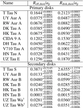
Table 3 reports the ratio betweenReff,dustandRdisk,dustmeasured for the disk around the primary stars and the observed separation between the two components of the multiple systems. These sep-arations are calculated from the fitted positions of the centers of the disks in our data, or obtained from the literature in the case only one component is detected (V710 Tau and DH Tau).
Manara et al.: Binaries in Taurus
0
200
400
Projected separation [au]
0
20
40
60
80
100
Radius 95% [au]
TTauB
UZTauW
R/a=0.3
R/a=0.2
R/a=0.1
TT
UY
RW
DK
HK
CI
DH
V7
HN
UZ
TT
UY
RW DK
HK
HN
UZ
UZ
Primary
Secondary
Fig. 14.Observed separation of the components in the multiple systems vs the measured radii of the individual disks. Only the first two letters of the names are reported to label the points. CI is for CIDA 9. The lines represent the ratios of radius to observed separation of 0.3 (solid line), 0.2 (dashed line), and 0.1 (dot-dashed line). TTau S is out of the plot to the top, but the fit is uncertain. UZ Tau W represents the values for the radii of the West components of the UZ Tau system, assuming only the distance between Wa and Wb.
smaller than 0.3 in our sample, with the only exception of the very uncertain radius measured for T Tau S. The typical ratio
Rdisk,dust/ap is .0.1, and only the West component of UZ Tau shows a value ofRdisk,dust/ap > 0.2. As discussed in the litera-ture (e.g., Papaloizou, & Pringle 1977; Artymowicz, & Lubow 1994; Rosotti & Clarke 2018), it can be analytically computed that tidal torques dominate over viscous ones outside a trunca-tion radius, which for a circular orbit is Rt ∼ 0.3·a, wherea is the semi-major axis of the binary orbit, with a dependence on the mass ratioq(see Fig. C.1).
Since statistically it is more probable to observe stars at apocenter of the binary orbit, as a very first approximation, we assume ap ∼ a, and therefore that the measured values of
Rdisk,dust/ap point to dust disk radii smaller than what would be expected from tidal truncation models, in line with the results of Cox et al. (2017), suggesting that either the binaries are on very eccentric orbits or that dust radii are smaller than gas radii by factors&2-3, probably due to a more effective drift of the dust probed by our 1.3 mm observations.
To further verify these possibilities we perform in the next sub-section a detailed comparison of our results with analytic models of tidal truncation.
5.2. Comparison with analytic predictions of tidal truncation
As described in App. C.1, starting from the work of Artymowicz, & Lubow (1994) a fit to the expected truncation radius can be derived as a function of the semi-major axis of the orbit (a) and the eccentricity (e) under the assumption that the disks and the binary orbit are co-planar (Eq. C.3). Combining Eq. C.3 with the fact that the exact analytic expression for the ratio between the semi-major axis and the projected separation is:
F= a ap
= 1−e2
1+e·cosν
q
1−sin2(ω+ν) sin2i
−1
, (7)
whereeis the eccentricity,νis the true anomaly,ω is the lon-gitude of periastron andiis the inclination of the plane of the orbit with respect to the line of sight, it is possible to obtain the following equation for the ratio of the truncation radius to the projected separation:
Rtrunc
ap
= 0.49·q
2/3
i
0.6·q2i/3+ln(q+q1i/3)
b·ec+0.88µ0.01·
· "
1−e2
1+e·cosν
q
1−sin2(ω+ν) sin2i
#−1
(8)
whereqi is the mass ratio (either q1 = M1/M2 or q2 = q =
M2/M1), and b and care the parameters derived in App. C.1 and tabulated in Table C.1, that depend on the disk viscosity, or equivalently on the Reynolds number,R.
These values ofRtrunc/aphave a minimum when the object is at apoastron (ω=0,ν=π), meaning whenap =a·(1+e), and a maximum at periastron (ω =ν=0), whenap =a·(1−e), at a given orbital inclination. The minimum ratio is found ati=0◦ and this ratio increases for higher orbital inclinations. Under the conservative assumption of face-on orbits (i=0◦), the two set of lines plotted in the following plots (see for example Fig. 15, for the specific case of RW Aur. Similar curves for the other sources in our sample are presented in Appendix C.2) are described by the equations:
Rtrunc
ap
= 0.49·q
2/3
i
0.6·q2i/3+ln(q+q1i/3)
b·ec+0.88µ0.01·(1+e)−1
Rtrunc
ap
= 0.49·q
2/3
i
0.6·q2i/3+ln(q+q1i/3)
b·ec+0.88µ0.01·(1−e)−1,
(9)
where the former refers to the truncation radius for an object located at apoastron, and the latter at periastron. Each line is plotted for three different values of the Reynolds number (R), as discussed in App. C.1.
0.00 0.25 0.50 0.75
Eccentricity
0.0
0.2
0.4
0.6
0.8
1.0
R
tru
nc
/a
p
RWAur
Re=10
4Re=10
5Re=10
6R95
R68
R95*2
R68*2
Fig. 15.Ratio of the truncation radius to the projected separation of the orbit as a function of eccentricity assuming the parameters of the RW Aur system and orbital inclinationi=0◦
. The two sets of black lines are the expectations from analytic models of tidal truncation (Eq. 9) each one calculated for three different values ofR (see legend). The set of three lines at the bottom is the estimate for an object observed at apoastron, the top ones at periastron. The red dashed and blue dot-dashed lines report the measured values ofRdisk,dust/apandReff,dust/apfor RW Aur A. respectively, while the red solid and blue dotted lines are a factor of two higher, corresponding to the assumed ratio of the gas to dust radius in the disk.
In general, it is to be expected that the eccentricity in these systems should be small for three considerations. First of all, values ofe∼1 would imply that at any passage at periastron the effects of tidal interaction on the disks would be massive, lead-ing to a severe truncation that would significantly shorten the disk lifetime and lead to a rapid disk dissipation (e.g., Clarke, & Pringle 1993). This effect of a close highly eccentric passage of the secondary is observed for example in the RW Aur system (e.g., Cabrit et al. 2006; Dai et al. 2015). Secondly, the orbital eccentricity may be uniformly random at formation, and decay with time (e.g., Bate 2018). Therefore, it is expected that eccen-tricities are typicallye<0.5, or less, for multiple systems in the Taurus region. Thirdly, observed distribution of eccentricities for main-sequence binary systems of low-mass stars show that the median eccentricity is∼0.3 (e.g., Duchêne, & Kraus 2013), and only less than 10% of the systems havee>0.6.
We thus explore here the eccentricities one would derive using as a value for the truncation radius the measured dust disk radii, eitherReff,dust orRdisk,dust, and an estimate of the gas disk radii taken to be two times larger than the dust radii. The lat-ter factor is chosen based on the median value obtained through the observation of disks in the Lupus star-forming region with ALMA (Ansdell et al. 2018). Although most of the disks ana-lyzed by Ansdell et al. (2018) are single, this is to date the largest sample of resolved disks observed both in the dust and the gas emission. A similar value for this factor between the gas and dust disk radius is also observed in the RW Aur system (Rodriguez et al. 2018) and in the older HD100453 system (van der Plas et al. 2019), but it could in principle be different in binaries, in general. Indeed, since this ratio is driven by several effects, including CO
optical depth and growth and drift of dust grains (e.g., Dutrey et al. 1998; Birnstiel, & Andrews 2014; Facchini et al. 2017; Trap-man et al. 2019), the effect on this ratio of an external truncation is still uncertain. It is also worth noting that this factor can be even larger than 5 in some extreme cases (Facchini et al. 2019).
We consider two different cases for the orbital inclination: (1) the conservative case where the binary orbit hasi =0◦and
(2) the case where the binary orbit is assumed to be coplanar with the primary disc. Note that for case (1) we still use the theoretical truncation radius obtained for coplanar discs, which again is a conservative choice.
Case 1: Face-on binary (i = 0◦). We show in Fig.
C.2-C.10 the comparison between the theoretical predictions and the measured values ofRdisk,dust/apfor all the sources in our sample. BothRdisk,dust/apandRdisk,gas/apare found to always be compat-ible with the expected values if the target is currently located at apoastron or between apoastron and periastron. This is ex-pected, as this is the position along the orbit where objects spent the largest amount of time. However, the inferred minimum val-ues of eccentricity are in general quite high (e > 0.5 in 9/11 cases) assuming the truncation radius to be equal to the dust disk radius. This is shown in Fig. 16, where the dust disk radius is estimated either as Reff,dust (upper panel) or Rdisk,dust (lower panel). Note that the estimated minimum eccentricities do not vary much when changing the definition of the dust radius. A more reasonable distribution of eccentricities is instead found if we assume that the truncation radii equal to twice the dust disk radius, as shown in Fig. 17, where again the upper and lower panels refer to the two choices for the dust radius.
Case 2: Binary coplanar with circumprimary disc.This
assumption is probably not representative of the reality since in many cases these two planes are not aligned in hydrodynamical simulations of star formation (e.g., Bate 2018) or in observations where disks are resolved and the orbit is constrained (e.g., Ro-driguez et al. 2018; van der Plas et al. 2019). In any case, also under this assumption, the derived orbital eccentricities are very high both assumingRtrunc=Rdisk,dust (e > 0.6 in 9/11 cases, see Fig. 18) or two timesRdisk,dust (e >0.5 in 7/11 cases, see Fig. 19).
6. Discussion
The analysis of the dust continuum emission in our sample of disks around stars in multiple stellar systems in Taurus shows that these disks are smaller in size than disks around single stars, that their outer edges present a more abrupt truncation than disks around single stars, and that very high orbital eccentricities are expected if we assume that the observed values of Rdisk,dust/ap correspond to the tidal truncation due to the binary.
The dust continuum emission probed by our observation is a tracer of the (sub-)mm dust grains in the disks, and these grains do not directly respond to the gas disk dynamics. Indeed, the location and emission profile of dust grains in disks depends on the details of how dust grains grow and drift in the disk (e.g., Testi et al. 2014) and by their opacity profile (e.g., Rosotti et al. 2019).
Manara et al.: Binaries in Taurus
TTau
UYAur
RWAur
DKTau
HKTau
CIDA9
DHTau
V710Tau
HNTau
UZTau
UZTauW
0.0
0.1
0.2
0.3
0.4
0.5
0.6
0.7
0.8
0.9
Eccentricity
R68%
TTau
UYAur
RWAur
DKTau
HKTau
CIDA9
DHTau
V710Tau
HNTau
UZTau
UZTauW
0.0
0.1
0.2
0.3
0.4
0.5
0.6
0.7
0.8
0.9
Eccentricity
R95%
Fig. 16.Minimum eccentricities obtained comparing the measured dust disk radii with the theoretical prediction of truncation assuming face-on orbital planes. The error bars are dominated by the difference in the models with different Reynolds numbers. The upper panel refers to the definition of dust radii as Reff,dust, while the lower panel refer to the definition of dust radii asRdisk,dust.
emission in disks around multiple stars could also be similarly interpreted. Indeed, dust radial drift has been shown to imply a sharp outer edge in disks (Birnstiel, & Andrews 2014), although this observed sharp outer edge could be an effect of the dust opacity profile (Rosotti et al. 2019). Work needs to be done to verify whether a sharp truncation in the gas disk implies smaller and more sharply truncated dust disks, as we observe here.
Another possibility is that the smaller observed sizes of disks in multiple systems is not an effect of disk evolution, instead it is the result of a smaller disk size in multiple systems at formation. Wide protostar binaries are found in simulations of star forma-tion (e.g., Bate 2018) as well in observaforma-tions. In the latter case the circumbinary disk is found to be large (∼300 au, Takakuwa
TTau
UYAur
RWAur
DKTau
HKTau
CIDA9
DHTau
V710Tau
HNTau
UZTau
UZTauW
0.0
0.1
0.2
0.3
0.4
0.5
0.6
0.7
0.8
0.9
Eccentricity
R68%
TTau
UYAur
RWAur
DKTau
HKTau
CIDA9
DHTau
V710Tau
HNTau
UZTau
UZTauW
0.0
0.1
0.2
0.3
0.4
0.5
0.6
0.7
0.8
0.9
Eccentricity
R95%
Fig. 17. Minimum eccentricities obtained assuming truncation radii equal to twice the measured dust disk radii and comparing with the the-oretical prediction of truncation assuming face-on orbital planes. The error bars are dominated by the difference in the models with different Reynolds numbers. The upper panel refers to the definition of dust radii asReff,dust, while the lower panel refer to the definition of dust radii as
Rdisk,dust.
et al. 2017; Artur de la Villarmois et al. 2018). Current work is thus not yet ready to constrain whether disks in multiple systems are small at the time of their formation.
TTau
UYAur
RWAur
DKTau
HKTau
CIDA9
DHTau
V710Tau
HNTau
UZTau
UZTauW
0.0
0.1
0.2
0.3
0.4
0.5
0.6
0.7
0.8
0.9
Eccentricity
R68%
TTau
UYAur
RWAur
DKTau
HKTau
CIDA9
DHTau
V710Tau
HNTau
UZTau
UZTauW
0.0
0.1
0.2
0.3
0.4
0.5
0.6
0.7
0.8
0.9
Eccentricity
R95%
Fig. 18.Minimum eccentricities obtained comparing the measured dust disk radii with the theoretical prediction of truncation assuming orbital planes co-planar with the primary disk. The error bars are dominated by the difference in the models with different Reynolds numbers. The upper panel refers to the definition of dust radii as Reff,dust, while the lower panel refer to the definition of dust radii asRdisk,dust.
to 5 or more (Facchini et al. 2019). Under the assumption that the analytic predictions of tidal truncation are correct, we can conclude that a factor of∼2 is needed also in binary systems to obtain values of orbital eccentricities more in line with expecta-tions.
7. Conclusions
We have presented here the analysis of our sample of 10 multiple systems in the Taurus star-forming region observed with ALMA in the 1.3 mm continuum emission at spatial resolution∼0.1200.
The sample, comprising 8 binaries and two triples, is part of a larger sample of disks in Taurus observed by our group (Long
TTau
UYAur
RWAur
DKTau
HKTau
CIDA9
DHTau
V710Tau
HNTau
UZTau
UZTauW
0.0
0.1
0.2
0.3
0.4
0.5
0.6
0.7
0.8
0.9
Eccentricity
R68%
TTau
UYAur
RWAur
DKTau
HKTau
CIDA9
DHTau
V710Tau
HNTau
UZTau
UZTauW
0.0
0.1
0.2
0.3
0.4
0.5
0.6
0.7
0.8
0.9
Eccentricity
R95%
Fig. 19. Minimum eccentricities obtained assuming truncation radii equal to twice the measured disk radii and comparing with the theo-retical prediction of truncation assuming orbital planes co-planar with the primary disk. The error bars are dominated by the difference in the models with different Reynolds numbers. The upper panel refers to the definition of dust radii asReff,dust, while the lower panel refer to the def-inition of dust radii asRdisk,dust.
et al. 2018, 2019). This allowed for a comparison between the properties of disks in multiple systems and disks around single stars.