Fast and Accurate Haplotype Inference
with Hidden Markov Model
Yi Liu
A dissertation submitted to the faculty of the University of North Carolina at Chapel Hill in partial fulfillment of the requirements for the degree of Doctor of Philosophy in
the Department of Computer Science.
Chapel Hill 2013
Approved by:
Wei Wang
Yun Li
Vladimir Jojic
Fernando Pardo Manuel de Villena
c 2013
Yi Liu
Abstract
YI LIU: Fast and Accurate Haplotype Inference with Hidden Markov Model
(Under the direction of Wei Wang and Yun Li)
The genome of human and other diploid organisms consists of paired chromosomes. The haplotype information (DNA constellation on one single chromosome), which is crucial for disease association analysis and population genetic inference among many others, is however hidden in the data generated for diploid organisms (including human) by modern high-throughput technologies which cannot distinguish information from two homologous chromosomes. Here, I consider the haplotype inference problem in two com-mon scenarios of genetic studies:
1. Model organisms (such as laboratory mice): Individuals are bred through prescribed pedigree design.
2. Out-bred organisms (such as human): Individuals (mostly unrelated) are drawn from one or more populations or continental groups.
Acknowledgements
First of all I would like to express my sincere thanks to my advisors, Drs. Wei Wang and Yun Li, for their continuous guidance and support, for being approachable anytime I had a problem, for explaining to me patiently even when I was in the “memoryless” state, and for giving me much freedom in working (and playing).
I had been very lucky to have chances to explore several different areas. I feel es-pecially fortunate to have worked with Drs. Fernando Pardo Manuel de Villena and Vladimir Jojic. Fernando has patiently taught me many basics of biology and helped me in linking computational methods to real biology problems; Vladimir introduced me to many optimization techniques and always inspired me through thoughtful questions. My thanks also go to other research collaborators and committee members for helpful dis-cussions on research and on completing my dissertation, William Valdar, Ethan Lange, Gary Churchill, Leonard McMillan, Xiang Zhang and all students (current and past) in the CompGen group and in the Li lab. I am very grateful to Qi Zhang for mentoring and helping me in many ways during my first year and my internships, to Zhaojun Zhang and Qing Duan for carrying out research together.
Table of Contents
List of Tables . . . xi
List of Figures . . . xiii
1 Introduction . . . 1
1.1 Background . . . 2
1.1.1 DNA and Haplotype . . . 2
1.1.2 Genotype . . . 3
1.2 Model Organisms from Prescribed Breeding . . . 3
1.3 Samples from Out-bred Human Populations . . . 5
1.4 Thesis Statement . . . 8
1.5 Contributions . . . 8
1.5.1 Model Organisms from Prescribed Breeding . . . 8
1.5.2 Samples from Out-bred Human Populations . . . 9
2 Efficient Genome Ancestry Inference in Complex Pedigrees with Inbreeding . . . 11
2.1 Introduction . . . 11
2.2 The Genome Ancestry Problem . . . 15
2.3.1 Modeling Inbreeding Generations . . . 16
2.3.2 Integrating the Inbreeding Model . . . 22
2.4 Modeling the Collaborative Cross . . . 25
2.4.1 The Breeding Scheme . . . 25
2.4.2 Modeling the Genome of G2Ik Generation . . . 26
2.5 Experiments . . . 27
2.5.1 Experiments on Simulated Data . . . 27
2.5.2 Experiments on Real CC data . . . 29
2.5.3 Running Time Performance . . . 33
2.6 Discussion . . . 33
3 High Definition Recombination Map in a Highly Divergent Mouse Population . . . 35
3.1 Introduction . . . 35
3.2 Materials and Methods . . . 37
3.2.1 The Genotype Data . . . 37
3.2.2 Haplotype Reconstruction and Recombination Inference . . . 38
3.3 Overview of the Recombination Map . . . 40
3.4 Sex Effect on Recombination . . . 42
3.5 Cold Regions . . . 44
3.5.1 Identification of Cold Regions in the G2I1 Population . . . 46
3.5.2 External Validation of Cold Regions . . . 47
3.5.3 Genomic Analysis of Cold Regions . . . 49
4 MaCH-Admix: Genotype Imputation for Admixed Populations . . . 51
4.1 Introduction . . . 51
4.2 Materials and Methods . . . 54
4.2.1 General Framework . . . 55
4.2.2 Piecewise IBS-based Reference Selection . . . 56
4.2.3 Ancestry-weighted Approach . . . 59
4.2.4 MaCH-Admix . . . 60
4.2.5 Datasets . . . 61
4.2.6 Methods Compared . . . 65
4.2.7 Measure of Imputation Quality . . . 65
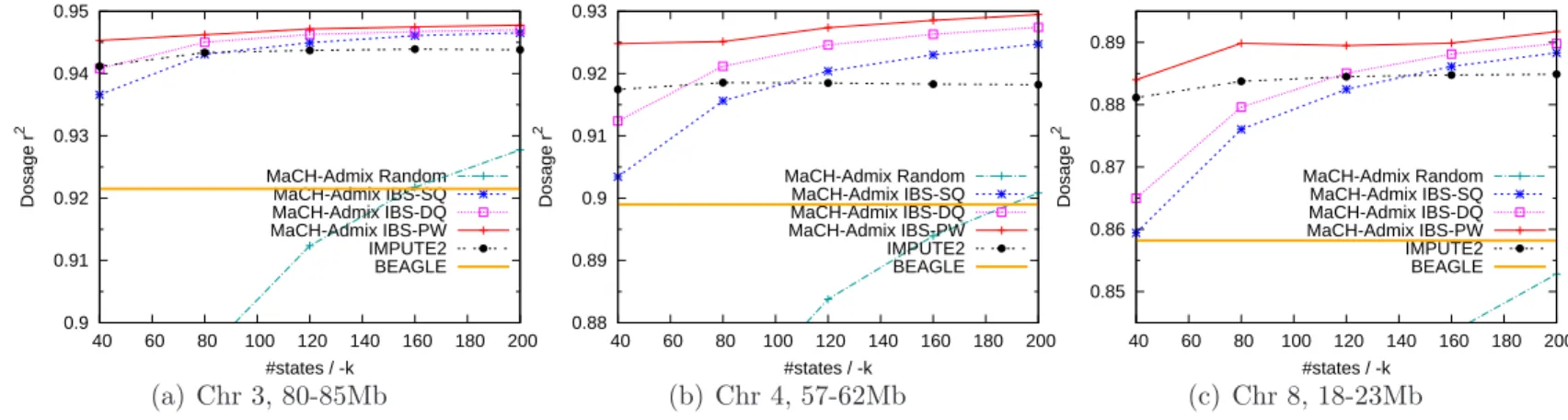
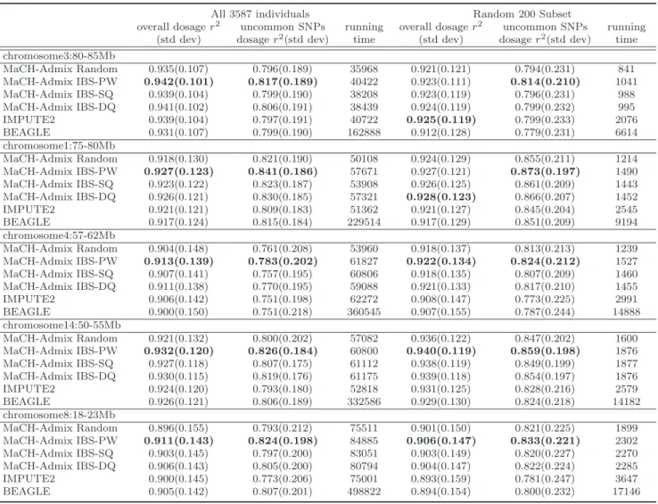
4.3 Results . . . 66
4.3.1 WHI-AA and WHI-HA with the 1000G Reference . . . 66
4.3.2 HapMap ASW and MEX with the 1000G Reference . . . 73
4.3.3 Imputation Performance with HapMap References . . . 75
4.3.3.1 WHI-HA and WHI-AA with HapMap references . . . 75
4.3.3.2 HapMap ASW and MEX with HapMap references . . . 75
4.3.4 Running Time . . . 79
4.4 Discussion . . . 83
5 Genotype Imputation of Metabochip SNPs in African Americans Using a Study Specific Reference Panel . . . 89
5.1 Introduction . . . 89
5.2.2 General Pipeline for Reference Construction and
Subsequent Imputation . . . 92
5.3 Results . . . 92
5.3.1 Genomewide Imputation . . . 92
5.3.2 Quality Estimate by Masking GWAS SNPs . . . 94
5.3.3 Quality Estimate by Masking Reference Individuals . . . 96
5.3.4 Overall Imputation Performance and Practical Guidelines . . . 102
5.3.5 Rare SNPs during Haplotype Reconstruction . . . 103
5.4 Discussion . . . 108
6 Conclusion . . . 114
6.1 Future Directions . . . 115
6.1.1 Model Organisms from Prescribed Breeding . . . 115
6.1.2 Samples from Out-bred Human Populations . . . 116
List of Tables
2.1 All Possible Transitions ofS(a), S(b) . . . 19
3.1 Summary of Identified Recombination Events in G2I1 Mice . . . 40
3.2 List of Cold Regions Identified . . . 48
4.1 Median Half Life ofr2 (in Kb) . . . . 63
4.2 Imputation Results of WHI-HA Individuals over Five 5Mb Regions with the 1000G reference . . . 71
4.3 Imputation Results of WHI-AA Individuals over Five 5Mb Regions with the 1000G reference . . . 72
4.4 Imputation Results of HapMap ASW & MEX Individuals over Five 5Mb Regions with the 1000G reference . . . 76
4.5 Imputation Results of WHI-HA Individuals over Five 5Mb Regions with the HapMapII reference . . . 77
4.6 Imputation Results of WHI-AA Individuals over Five 5Mb Regions with the HapMapII reference . . . 78
4.7 Imputation Results of 49 ASW Individuals Over All Five Short Regions . . . 80
4.8 Imputation Results of 49 ASW Individuals Over All Five Short Regions . . . 81
4.9 Imputation Results of 50 MEX Individuals Over All Five Short Regions . . . 82
5.2 Average Rsq and Dosage r2 by MAF, Estimated by Masking
100 Reference Individuals . . . 101
5.3 Effect of Including Rare Variants for Reference Panel
Construction . . . 106
5.4 Effect of Including Rare Variants for Haplotype Reconstruction
among Target Individuals . . . 107
5.5 Effect of Including/Excluding the 100 Masked Reference
Individuals during Reference Haplotype Reconstruction . . . 108
5.6 Average Rsq and Dosage r2 by MAF, Estimated by Masking
List of Figures
1.1 Toy example of two chromosomes with haplotypes defined
on three sites containing variations . . . 2
2.1 Inhertiance indicators of an inbreeding process . . . 17
2.2 Comparison of predicted probabilities and observed probabilities from simulations . . . 23
2.3 Collaborative Cross breeding scheme and the corresponding inheritance indicators . . . 26
2.4 Comparison of error rates of GAIN, MERLIN and HAPPY on simulated data sets . . . 28
2.5 Proportion of probabilities assigned to wrong ancestry by GAIN and HAPPY on simulated data sets . . . 29
2.6 The difference in ancestry estimated by GAIN and HAPPY . . . 31
2.7 Two examples of ancestry inference by GAIN and HAPPY . . . 32
2.8 Average running time of GAIN, HAPPY and MERLIN . . . 33
3.1 The CC funnel pedigree toG2I1 generation . . . 37
3.2 Distribution of recombination interval length in log-scale . . . 41
3.3 Recombination map length of autosomes by Prdm9 allele and gender . . . 43
3.4 Distribution of recombination events along the autosomes in female and male meioses . . . 44
4.1 A cartoon illustration of two scenarios where three
IBS-based selection methods perform differently . . . 58
4.2 Median r2 half-life value of 5Mb windows on 5 chromosomes . . . . 64
4.3 Imputation of 3587 WHI-HA with the 1000G reference panel . . . 68
4.4 Imputation of 8421 WHI-AA with the 1000G reference panel . . . 69
4.5 Minor Allele Frequency (MAF) distribution of SNPs in WHI-AA and WHI-HA. . . 73
4.6 Imputation of 49 HapMap ASW and 50 HapMap MEX individuals with the 1000G reference panel . . . 74
4.7 Imputation quality of ASW with HapMapII CEU+YRI+ LWK+MKK reference panel . . . 79
5.1 Reference construction and imputation pipeline using a study-specific reference panel . . . 93
5.2 Imputation accuracy by chromosome for 2% randomly masked GWAS SNPs . . . 95
5.3 Rsq by dosage r2 for 2% randomly masked GWAS SNPs . . . . 97
5.4 MAF distributions of Affymetrix 6.0 and Metabochip SNPs . . . 98
5.5 Physical spreading of Affymetrix 6.0 and Metabochip SNPs . . . 99
5.6 Imputation accuracy by chromosome for Metabochip SNPs (estimated by masking 100 reference individuals) . . . 99
5.7 Accuracy and calibration of imputation . . . 100
Chapter 1
Introduction
Recent technological advances in life sciences have generated massive amounts of data which enables accurate analyses of genome ancestry, recombination properties, complex disease susceptibility, and drug response, among many others. However, it is often the haplotype information that is more powerful in such analyses than the data directly obtained from high-throughput technologies such as genotyping. Therefore, how to re-construct haplotype information from massive amount of raw data and make related inference based on recovered haplotype information are key problems in genetic studies and pose serious computational challenge.
In this thesis, I have developed statistical methods and computational tools that, by reconstructing haplotype information, generate accurate inferences for important prob-lems including genome ancestry and imputation. My methods, based on Hidden Markov Model (HMM), can efficiently handle large scale datasets from two common settings in modern genetic studies:
1. Model organisms (such as laboratory mice): Individuals are bred through prescribed pedigree design.
1.1
Background
1.1.1
DNA and Haplotype
Diploid species, which include nearly all mammals, carry paired homologous chromo-somes, one inherited from each parent. A haplotype refers to the DNA sequence data from one of the paired chromosomes. Within the same species, DNA sequences are largely identical differing only slightly among individuals. Thus haplotypes are often defined only at positions with sequence variations. Figure 1.1 shows a toy example of two chromosomes with 15 sites and the two haplotypes defined at sites with variations.
Figure 1.1: Toy example of two chromosomes with haplotypes defined on three sites containing variations
1995]. In these problems, even if reconstructed with uncertainty, haplotype information could lead to significantly increased power in inferences.
Even though it is possible to obtain haplotype information of diploid organisms di-rectly from biological experiments, it is generally expensive and cannot scale to large sam-ple size. On the contrary, modern high-throughput genotyping technologies can generate accurate genotype readings on hundreds of thousands of markers at much lower cost. It is thus valuable to conduct analysis by reconstructing haplotypes based on genotype inputs.
1.1.2
Genotype
Modern high-throughput genotyping technologies generate genotype readings on a pre-selected set of genetic markers. The set of markers can be defined by standard commercial platforms (e.g., Affymatrix 6.0, Illumina 1M), or customized by researchers (e.g., Yang
et al. [2009]). Each genotype reading, or simply genotype, is an unordered combination of two alleles from paired chromosomes. In other words, genotypes are unable to dis-tinguish between the two haplotypes of a diploid organism. It cannot tell which allele is from which haplotype.
In this dissertation, I consider how to bridge the gap between genotype data and desired genetic analyses by reconstructing haplotypes probabilistically. Here, I consider two common settings in genetic studies and related inference problems specific to settings.
1.2
Model Organisms from Prescribed Breeding
mixed in each generation. A DNA sequence of any descendant organism is a mosaic of its founders’ DNA segments.
One example of such resources is the international Collaborative Cross (CC) project which is a major effort in the mouse research community and has been under development for more than 10 years [Threadgill and Churchill, 2012]. The CC project consists of hundreds of independently bred, recombinant-inbred mouse lines generated through a funnel breeding design (Figure 2.3). Each line has more than 20 expected generations. High-density genotype data of the CC resources not only provide opportunities for fine-resolution quantitative trait locus (QTL) studies, but also facilitate exciting new research areas such as the inference of genetic networks underlying phenotypic traits in mammals. Among many analyses of interest, a core problem is to discover the founder attribution to genomes in subsequent generations. That is to say, given a descendant organism in the resource, I want to find out which part of its DNA sequences is inherited from which founder (genome ancestry in founders). The genome ancestry information provides direct knowledge of historical recombination events and opportunities for error detection and imputation. It also enables downstream analyses such as measuring strain effect in quantitative traits.
Inference of genome ancestry involves resolving the potential inheritance flow at all markers of interest. This naturally requires the resolution of haplotype information as haplotypes correspond to the variants inherited together in the breeding process. It is straightforward to show that, in a pedigree withnnon-founders andmmarkers of interest, there are 2mn possible inheritance configurations even if one assumes known founder
haplotypes and only bi-allelic markers. In a typical CC pedigree, there could be more than 40 mice and the enormous search space presents a major computational challenge. The commonly favored pedigree-based haplotyping methods [Kruglyak et al., 1996;
which far exceeds other parameters. However, these methods are limited to pedigrees of moderate size since the running time grows exponentially with pedigree size. When they are applied to the genotype data from CC, the search space becomes extraordinarily large due to the large pedigree structure with many untyped intermediate generations. Other pedigree-based haplotyping methods include MCMC sampling methods [Sobel and Lange, 1996; Jensen and Kong, 1999], whose computing time can be substantial when applied to a large number of tightly linked markers, and rule-based methods [Qian and Beckmann, 2002; Li and Jiang, 2005], which have a crude approximation by minimiz-ing recombinations in pedigree. More computationally efficient approaches for solvminimiz-ing the genome ancestry problem have ignored pedigree information, including the breed-ing scheme. Examples include the combinatorial optimization approach by Zhang et al. [2008] and the HMM-based method in HAPPY [Valdaret al.,2006; Mott et al., 2000], a QTL mapping tool suite for association studies. All ancestry compositions are considered possible in the two methods. While breeding design does not determine the locations of recombination, it places important constraints on the possible ancestry choices at a single marker and at neighboring markers. Therefore, incorporating breeding design information would lead to more accurate inference.
1.3
Samples from Out-bred Human Populations
The ultimate goal of almost all genetic research is to understand genetic mechanisms in humans. Therefore, tremendous efforts have been spent on investigating human samples directly. In contrast to model organisms where breeding is often designed and controlled, humans are out-bred and the genetic data of founders are generally unavailable. Since
genetic information, and use of unrelated individuals is that individuals studied tend to share only short haplotype segments (e.g., several hundred Kbs) of their chromosomes. This is further confounded by the presence of population and sub-population structure. Reconstruction of haplotype in such out-bred populations is therefore challenging but of great importance in genetic studies.
By aligning samples under study to samples in existing studies (e.g., HapMap and 1000 Genomes projects [The International HapMap Consortium,2010;The 1000 Genomes Project Consortium, 2012]), researchers can identify the shared haplotype segments among samples. Consequently, one can not only recover the sporadic technological fail-ures in genotypes, but also impute the markers that are untyped in individual studies but typed in reference samples. This genotype imputation technique greatly improves the marker density and analysis power of individual studies.
Moreover, as the typical small to moderate effect of individual genetic variant on complex trait entails large sample size, collaborative efforts that pool information across multiple studies are typically taken to enhance the statistical power for detecting causal variants. In these collaborative efforts, samples from different studies are typically geno-typed at different sets of markers because different commercially available genotyping platforms are used. The commonly used genotyping platforms have a small fraction of markers in common (∼10% is typical between platforms from two different companies). Restricting analysis to markers in common leads to much reduced marker density and huge loss of information. Imputation of markers untyped in individual studies greatly facilitates the integration of samples across studies (meta-analysis) .
or the 1000 Genomes Projects [The International HapMap Consortium, 2010; The 1000 Genomes Project Consortium, 2010]. The wealth of literature using genotype imputa-tion has focused on using external reference panels (for example, phased haplotypes from the HapMap and 1000 Genomes projects), largely in individuals of European ancestry, for inference of genotypes at common (minor allele frequency [MAF] > 0.05) genetic markers. Several important issues have not been adequately addressed including the utility of study-specific reference, accommodation of increasingly large reference panels, performance in admixed populations, and quality for less common (MAF ∼ 0.005-0.05) and rare (MAF < 0.005) variants. These issues only recently became addressable with Genome-Wide Association (GWA) follow-up studies using dense genotyping or sequenc-ing in large samples of non-European individuals.
Also, little methodological work exists for imputation in admixed populations, such as African Americans and Hispanic Americans, which comprise more than 20% of the US population. Admixed populations offer a unique opportunity for gene mapping, but also impose challenges for imputation. To efficiently benefit from emerging large reference panels, one key issue to consider is on how to traverse the reference space harboring the most probability mass with minimum computational efforts. In modern genotype impu-tation framework, this corresponds to the selection of effective reference panels. Existing works often focused on constructing a pre-defined reference panel prior to running the imputation engine. Such methods (e.g., a cosmopolitan panel [Hao et al., 2009; Li
et al., 2009; Shriner et al., 2010] or a weighted combination panel [Egyud et al., 2009;
tationally, for example, through integration of the former approach within (rather than prior to) the hidden Markov model, or through more elegant heuristics.
1.4
Thesis Statement
Genetic analyses of model organism resources and out-bred populations can be achieved by reconstructing haplotype information implicitly or explicitly via HMM. By applying effective state-space pruning strategies, I present haplotype-based inference algorithms that can scale to large datasets without compromising accuracy. Application to CC mouse data leads to new biological discovery of properties of recombination events. Case study on Women’s Health Initiative (WHI) metabochip data leads to generalizable quality control guidelines for imputation analysis.
1.5
Contributions
In this section, I briefly summarize the contributions presented in subsequent chapters.
1.5.1
Model Organisms from Prescribed Breeding
polymor-phism (SNP) data with complex breeding design. Experiments show that, GAIN generates accurate results efficiently on data that cannot be handled by existing pedigree haplotyping software. Compared with HAPPY [Mott et al., 2000], which does not model pedigree structure, GAIN substantially reduces ambiguities in an-cestry inference.
• In Chapter 3, I generate a new linkage map of the laboratory mouse genome using GAIN described in previous chapter. The map is built with the recombination and ancestry information inferred from the genotypes of 237 male-female sibling pairs. Exploiting the large number of recombination events (n∼22,000), the high precision in mapping each event (∼35kb) and the unique characteristics of the CC mice, I provide a new and powerful look at the effects of sex, strain and genotypes at polymorphic loci of interest (e.g., thePrdm9 gene) on recombination. In addition to an extended catalog of sex and strain specific hotspots, I report the presence of cold regions for recombination with striking distributions and genomic characteristics.
1.5.2
Samples from Out-bred Human Populations
various sensible approaches for imputation in admixed populations and presents a comprehensive comparison.
Chapter 2
Efficient Genome Ancestry Inference
in Complex Pedigrees with
Inbreeding
2.1
Introduction
originate as mutations, which are rare events within a vast genome. It is therefore con-venient to encode a SNP allele as a binary value and represent haplotypes as binary sequences. Modern high-throughput genotyping technologies are unable to distinguish between the two haplotypes of a diploid organism. Instead, a genotype sequence is mea-sured where, at each SNP site, one of three possibilities is observed ({00,01,11}, since 10 cannot be distinguished from 01).
Using the genotype representation for DNA sequences, the genome ancestry problem estimates the origin of each genotype from a descendant’s sequence given the genotype sequences of its distant founders. To achieve high resolution, dense SNP markers are used ( tens of thousands on each chromosome ). Knowledge of genotype’s ancestry is particularly useful in many problems such as studying the structure and history of haplo-type blocks [Gabrielet al.,2002;Zhang et al., 2002;Schwartz et al., 2004], and mapping quantitative trait loci (QTLs)[Valdar et al., 2006; Mott et al., 2000]. In these studies, a probabilistic interpretation is favored over discrete solutions, due to the prevalence of ambiguities and measurement errors.
size. MCMC sampling methods [Sobel and Lange, 1996; Jensen and Kong, 1999] have been proposed to address larger pedigrees. But their computing time can be substan-tial when applied to a large number of tightly linked markers. Other efforts include rule-based methods [Qian and Beckmann, 2002;Li and Jiang,2005] which approximates a solution by minimizing recombinations in the pedigree (MRHC). PedPhase [Li and Jiang, 2005], which employs an effective integer linear programming (ILP) formulation, has been widely used in solving the MRHC.
Current haplotyping methods for pedigrees are incapable of solving the genome ances-try problem in animal resources for the following reasons: 1) Pedigrees of model animal resources often contain large number of generations to ensure diversity and reproducibil-ity. 2) None or few of the intermediate generations are genotyped due to the size of the resources. 3) A large number of dense markers are genotyped to achieve fine resolution. As a concrete example, more than one thousand lines have been started in the Collabo-rative Cross project [Churchill et al., 2004; The Collaborative Cross Consortium, 2012]. Each line is expected to undergo at least 23 generations before reaching 99% inbred. Hundreds of mice of various generations were genotyped, but on average only few are from the same line. The missing genotypes make the search space extraordinarily large. Other computationally efficient approaches for solving the genome ancestry problem have largely ignored the breeding scheme. While breeding design does not determine the locations of recombination, it often places constraints on the possible ancestry choices at a single site and at neighboring sites. The genome ancestry problem was modeled as a combinatorial optimization problem in [Zhang et al., 2008]. By minimizing recombi-nations, discrete solutions are generated. Mott et al. has proposed an approach using Hidden Markov Model (HMM) for ancestry inference in HAPPY [Valdar et al., 2006;
There have also been many efforts to analyze pedigree by identifying symmetries in HMM state space [Donnelly,1983;McPeek, 2002;Browning and Browning,2002;Geiger
et al.,2009]. The states are then grouped to accelerate the calculation. However, finding the maximal grouping is non-trivial. In real-world problems, only obvious symmetries such as founder phase and chain structure in pedigree can be best utilized.
Besides model organisms, the genetic ancestry problem has been studied for human individuals that have recently been admixed from a set of isolated populations, instead of a set of founders[Tang et al., 2006; Sundquist et al., 2008; Sankararamanet al., 2008;
Pa¸saniuc et al., 2009]. In this problem, pedigree structure is usually not present (unre-lated individuals) or the size of pedigree is small. Efficient methods have been developed to handle large-scale datasets[Tang et al., 2006; Sundquist et al., 2008; Sankararaman
et al., 2008].
2.2
The Genome Ancestry Problem
Given a pair of chromosomes, consider L SNP markers ordered by their chromosomal locations. For each SNP site, we use 0 and 1 to encode the two possible values. The genotype at each site is the unordered combination of corresponding alleles from both chromosomes, which can assume one of three values: 00, 01, 11. A genotype sequence is a genome-ordered set of genotypes denoted as: G=g1...gl...gL,(gl ∈ {00,01,11}). A
hap-lotype H=h1...hl...hL consists of alleles from one of the chromosomes wherehl ∈ {0,1}.
Consider a pedigree containing a set of foundersF S ={F1, ..., FN}and a descendant
of interest. I denote the set of founder genotype sequences by {GF1, ..., GFN}, all of which are given. Given the genotype sequence,GD, of the descendant generated through
the pedigree structure, its genome ancestry is to be determined. Every genotype gl in
GD inherits its alleles from two founders, say FA and FB. I refer to the founder pair
(FA, FB) as the genome ancestry at site l of genotype sequence GD. I want to estimate,
for every SNP site l, the probability P(Ancestry(gl) = (FA, FB)) for every founder pair
(FA, FB)∈F S×F S. Note that founder pairs are unordered ((FA, FB) = (FB, FA)), and
it is possible that FA = FB.
2.3
Modeling Inheritance in Pedigree
I start from the standard Lander-Green approach to model a pedigree: At each SNP site, an inheritance indicator is used to indicate the outcome of each meiosis. These inheritance indicators together form the inheritance vector. Since a child haplotype inherits its allele from either the paternal or maternal sequence, an inheritance indicator is a binary variable. For a pedigree withnnon-founder animals, there are 2×ninheritance indicators at each site. Hence, the inheritance vector at site l, vl, can be defined as a
inheritance flow at site l of all animals in the pedigree. When SNP markers are dense enough, one can assume at most one recombination between two sites in generating one haplotype. If a recombination happens between site l and l+ 1, the corresponding inheritance indicator will have different states for the two sites. Hence, to measure the number of recombinations between l and l + 1 in the whole pedigree, one can count the difference in bits between vl and vl+1. The probability of having d recombinations between l and l+ 1 is θd(1−θ)2n−d, where θ is the recombination fraction.
The length of inheritance vector grows linearly with the number of animals in the pedi-gree and this causes exponential growth in the number of possible inheritance patterns. Considering the fact that full pedigree analysis is computationally intractable, I overcome the issue by modeling important sub-structure in breeding systems as a shortcut to effi-cient computation. My first natural choice of sub-structure is inbreeding: 1) Inbreeding is often used in model animal resources to generate genetically diverse and/or reproducible descendants. 2) Inbreeding is often carried out for many generations and each generation elongates the inheritance vectors by 4 bits. Hence, if a pedigree involves inbreeding, the inbreeding generations often account for most of the computational complexity. I seek an aggregated inheritance indicator to replace the collection of many inheritance indicators in the inbreeding process. Such an aggregated indicator can be encoded in much shorter length and incorporated into the inheritance vector. If the state and transition proba-bility of the aggregated indicator can be modeled efficiently, full pedigree analysis will become feasible on these animal resources. In the next section, I explain how inheritance in inbreeding generations can be modeled as an aggregated indicator.
2.3.1
Modeling Inbreeding Generations
(a) (b)
Figure 2.1: (a) Lattice of binary inheritance indicators representing the inheritance pat-tern of an inbreeding process at a single site. (b) An equivalent quapat-ternary indicator representation
2.1(a). I denote the beginning generation of inbreeding as generationI0. Observe that, at each site, because of the symmetry of inbreeding structure, the four alleles at generation I0 have equal probabilities to be passed down to any haplotypes after I1. Thus, for a descendant haplotype at generation Ik (k > 2), I can simply replace the lattice of binary
inheritance indicators by a single quaternary indicator. Each choice of the quaternary indicator has 1/4 probability. Two quaternary indicators are needed for the two hap-lotypes of a Ik descendant (Figure 2.1(b)). However, the two quaternary indicators are
not independent as the two haplotypes share the same inbreeding history until Ik−1. To
model this dependency between the two quaternary indicators, I find out the transition events and probabilities of the pair of indicators. The grouped pair is then used as an aggregated inheritance indicator as discussed above.
I label the four I0 haplotypes as 1,2,3,4. I then denote bya, bthe two Ik descendant
haplotypes and S(al), S(bl) are their I0 sources at site l, i.e., S(al), S(bl) ∈ {1,2,3,4}.
adjacent sites, land l+ 1, all the possible transitions fromS(al), S(bl) to S(al+1), S(bl+1) (Table 2.1).
Note that:
PEE0+PEN1+PEE2+PEN2 =P(S(al) =S(bl)) =
PEE0+PEE2+PN E1+PN E2 =P(S(al+1) =S(bl+1))
and
PN E1+PN N0+PN N1+PN N2+PN E2 =P(S(al)6=S(bl)) =
PEN1+PEN2+PN N0 +PN N1+PN N2 =P(S(al+1)6=S(bl+1))
The prior probability P(S(al) = S(bl)) at any site l is called the inbreeding coefficient
[Wright, 1922]. To calculate the probability, let ICk denote the inbreeding coefficient at
generation Ik. ICk can be computed recursively using ICk = k−2 X
j=0 (1
2)
k−j
Site l Possible Transitions Site l+ 1 Denote By
S(al) =S(bl)
NeitherS(a) or S(b) transitions. S(al+1) =S(bl+1) PEE0
EitherS(a) or S(b) transitions, but not both. S(al+1)6=S(bl+1) PEN1
BothS(a) and S(b) transition to same value. S(al+1) =S(bl+1) PEE2
Both S(a) and S(b) transition, but to different values. S(al+1)6=S(bl+1) PEN2
S(al)6=S(bl)
Neither S(a) norS(b) transitions. S(al+1)6=S(bl+1) PN N0
EitherS(a) or S(b) transitions, but not both. S(al+1) =S(bl+1) PN E1
S(a) and S(b) become equal after the transition.
EitherS(a) or S(b) transitions, but not both. S(al+1)6=S(bl+1) PN N1
S(a) and S(b) remain different after the transition.
Both S(a) andS(b) transition. S(al+1)6=S(bl+1) PN N2
S(a) and S(b) remain different after the transition.
Both S(a) andS(b) transition. S(al+1)6=S(bl+1) PN E2
S(a) and S(b) become the same after the transition.
Table 2.1: All possible transitions of S(a), S(b). Each type of transition is denoted by 3 characters. First two letters indicate the equality of S(a), S(b) before and after the transition. Then followed by a digit indicating the number of transitions inS(a), S(b).
Next, I derive the probabilities in Table 2.1. Consider that any transition in S(a) or S(b) is caused by one or more recombinations in the inbreeding process (Figure 2.1(a)). My calculation is based on the assumption that the recombination fraction, θ, is rea-sonably small. Hence, for any haplotype c at generationIj (1≤j≤k), I assume that any
single transition in S(c) is solely caused by one recombination in generating cor its an-cestor haplotypes. In other words, a single transition in S(c) is not the result of multiple recombinations in the pedigree. My assumption is generally true for dense SNP markers where θ is usually well below 0.001. Under the assumption, if a transition in S(c) is caused by a recombination in generating c itself, I define this to be a lead transition. Intuitively, a lead transition is one not inherited from its ancestors. A lead transition in c will change the I0 source of c and all descendant haplotypes inheriting the transition. A lead transition is only possible when the two parental haplotypes of c have different I0 sources. Hence, between two sites, a haplotype at generation j has a lead transition with probability θ ×(1 −ICj−1).
With the inbreeding coefficients calculated, I can derive the marginal probability of ob-serving transition in one of theIkhaplotypes,P1T =P(S(al)6=S(al+1)) =P(S(bl)6=S(bl+1)). Without loss of generality, I consider P(S(al)6=S(al+1)) for haplotype a. S(a) will tran-sition if a itself or any of its ancestor haplotypes has a lead transition. At generation k, the lead transition happens with probability θ×(1−ICk−1). For generation k−1,
there are 2 possible ancestor haplotypes, each with 12θ×(1−ICk−2) chance of causing
a transition in S(a). For each generation j from 1 to k −2, there are 4 possible ances-tor haplotypes with probability 1
4θ ×(1−ICj−1). Consider that, at one site, any two
haplotypes from the same generation cannot both be the ancestor of a. Thus, for any generation j, the expected probability of causing transition in S(a) is θ ×(1−ICj−1).
Under my assumption,P(S(al)6=S(al+1)) can be expressed by 1−
k
Y
j=1
(1−θ×(1−ICj−1)).
some previous generation is the common ancestor ofa, band chas a lead transition. The probability of c at generation j being the common ancestor of a and b is 1
4ICk−j. The
probability thatchas a lead transition is θ×(1−ICj−1). Again, consider the fact that,
at one site, any two haplotypes from the same generation cannot both be the common ancestor of a and b. Thus, the probability of EE2 event caused by lead transition at Ij
(1≤j≤k−2) is θ×(1−ICj−1)ICk−j. Assuming a small θ, PEE2 can be calculated by 1−
k−2 Y
j=1
(1−θ×(1−ICj−1)ICk−j).
Lastly I consider the probability PN N1. To simplify my discussion, assume that the transition happens in S(a) (i.e. S(al)6=S(al+1)) and it inherits a lead transition in hap-lotype c of generation j. Since S(al), S(al+1) and S(bl) all have different I0 ancestry, alleles from at least 3 distinctI0 haplotypes should be observed at generation j−1. Let
PDistinct(m, j) be the probability of observing exactly m distinct I0 alleles at generation
j. PDistinct(3, j) and PDistinct(4, j) can be computed recursively using:
PDistinct(4, j) =
1
4PDistinct(4, j−1)
PDistinct(3, j) =
1
2PDistinct(3, j−1) + 1
2PDistinct(4, j−1)
Then, PN N1 is the probability that (1) at least 3 distinct I0 alleles are present at gen-eration j −1 and (2) a’s ancestor c at generation j has a lead transition between sites l and l + 1 which is inherited by a (3) before and after transition, the I0 source of c is different from that of b.
rapidly and PN N2, PN E2, PEN2 are much smaller than P(S(al)6=S(bl)). With P1T, PEE2 and PN N1 derived, I can easily solve all the rest probabilities in Table 2.1:
PN E1 =PEN1 = 1
2(2×(P1T −PEE2)−PN N1)
PEE0 =ICk−PEE2−PEN1
PN N0 = 1−ICk−PN E1−PN N1
PN N2, PN E2, PEN2 are approximated by a small probabilityPN E1×PN E1. I use simu-lation to validate the probabilities derived above. The results are shown in Figure 2.2. Forθ around 0.01, my method gives reasonably close approximation. Forθ below 0.001, my method is very accurate. The recombination fraction between dense SNP markers is usually well below 0.001.
So far I have derived all event probabilities in Table 2.1. The transition probability from (S(al), S(bl)) to (S(al+1), S(bl+1)) is the corresponding probability in Table 2.1 conditioned on P(S(al) = S(bl)) or P(S(al)6=S(bl)).
2.3.2
Integrating the Inbreeding Model
I have argued that each inbreeding process can be modeled by two quaternary indicators and their transition probabilities can be accurately approximated when θ is small. It is then straightforward to integrate the inbreeding model into the original Lander-Green model. I encode the two quaternary indicators using 4 binary bits in the inheritance vector. Consider a pedigree containing i inbreeding processes and n′
other members not involved in inbreeding. The inheritance vectorvlat every sitelnow has length 2×n
′
+4×i. Each possible realization ofvl is a hidden state in HMM. The transition probability from
0 0.1 0.2 0.3 0.4 0.5 0.6 0.7 0.8 0.9 1
5 10 15 20
Probability Inbreeding Generation θ=0.0001 θ=0.001 θ=0.01 (a) 0 0.0005 0.001 0.0015 0.002 0.0025
5 10 15 20
Probability Inbreeding Generation θ=0.0001 θ=0.001 (b) 0 0.001 0.002 0.003 0.004 0.005 0.006
5 10 15 20
Probability
Inbreeding Generation θ=0.0001
θ=0.001
(c)
Figure 2.2: Comparison of predicted probabilities and observed probabilities from 10000000 simulations. The data points in the figures are observed probabilities from sim-ulations. The curves are derived from my formulas. (a) Predicted and simulatedPEE0 for θ = 0.01,0.001,0.0001. (b) Predicted and simulated PEN1 = PN E1 for θ = 0.001,0.0001.
(c) Predicted and simulated PEE2 forθ= 0.001,0.0001. I do not plot the case of θ= 0.01
P(vl|GD) =
P(GD|vl)P(vl)
P(GD)
= P(g1, ..., gl|vl)P(gl+1, ..., gL|vl)P(vl) P(GD)
= P(g1, ..., gl, vl)P(gl+1, ..., gL|vl) P(GD)
= α(vl)β(vl) P(GD)
where
α(vl) = P(g1, ..., gl, vl)
β(vl) = P(gl+1, ..., gL|vl)
α(vl) and β(vl) can be solved recursively:
α(vl+1) =
X
vl
α(vl)P(vl+1|vl)P(gl+1|vl+1)
β(vl) =
X
vl+1
β(vl+1)P(vl+1|vl)P(gl+1|vl+1)
P(GD) is obtained from the calculated α(vl) and β(vl) at any site l:
P(GD) =
X
vl
α(vl)β(vl)
The genome ancestry at site l is, for every founder pair (FA, FB),
P(Ancestry(gl) = (FA, FB)) =
X
vl
P(vl|GD)
Note that, if I place the bits of quaternary indicators at the end of inheritance vec-tor, the recursive calculation of α and β can still greatly benefit from the Elston-Idury algorithm [Idury and Elston, 1997].
2.4
Modeling the Collaborative Cross
The Collaborative Cross (CC) [Churchillet al.,2004;Chesleret al.,2008;The Collabora-tive Cross Consortium, 2012] is a large panel of reproducible, recombinant-inbred mouse lines proposed by the Complex Trait Consortium. Over a thousand of mouse lines have been started among which several hundred lines are kept inbreeding. All mouse lines are generated using eight genetically diverse founders via a common breeding scheme designed to randomize the genomic contribution of each founder. It provides an ideal platform for testing my approach.
2.4.1
The Breeding Scheme
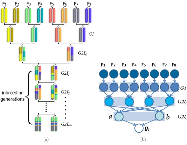
CC mice are derived from 8 fully inbred founders using the 8-way funnel breeding scheme shown in Figure2.3(a). The chromosomes of the eight founders (shown in different colors) are combined by two generations of crosses (labeled G1 and G2I0), followed by at least 20 inbreeding generations (G2I1 to G2I∞).
(a) (b)
Figure 2.3: (a) Collaborative Cross breeding scheme: An example derivation of chro-mosomes by recombining chrochro-mosomes from 8 ordered founders. G1 and G2I0 are two
generations of crosses. G2I1 to G2I∞ are multiple generations of inbreeding. (b) The inheritance indicators used to represent the inheritance flow at a SNP site.
2.4.2
Modeling the Genome of
G
2
I
kGeneration
In a CC pedigree, any recombination in the formation of G1 haplotypes can be virtu-ally ignored since all founders are fully inbred. Hence, at each SNP site, I only need 4 inheritance indicators for G2I0 haplotypes and 2 quaternary indicators for the two haplotypes in a resulting G2Ik descendant. The structure of the inheritance indicators
is shown in Figure 2.3(b).
G2I1 mice are an exception which only involve one generation of inbreeding. For a
This becomes a standard Lander-Green model and it can be seen that the two G2I1 haplotypes are restricted to be from the left and right half of the funnel respectively.
2.5
Experiments
In this section, I evaluate the proposed model on both simulated data and real CC geno-type data. I implement my model GAIN (Genome Ancestry with INbreeding) for CC using C++. GAIN is compared with MERLIN [Abecasis et al.,2001] and HAPPY [Mott
et al.,2000]. MERLIN is a widely used pedigree analysis software based on Lander-Green algorithm and can handle large number of markers. HAPPY is a QTL mapping tool suite and can analyze genome ancestry based on only founder and descendant genotype data, i.e., it ignores pedigree structure. Both software estimate the genome ancestry directly or indirectly.
2.5.1
Experiments on Simulated Data
As ground truth is generally unavailable for real data, I evaluate the accuracy of genome ancestry analysis using simulated data. I simulate the genotype of a G2Ik mouse by
recombining real CC founder haplotypes according to the CC pedigree structure. Given the founder genotypes, the founder haplotypes can be obtained trivially since all founders are fully inbred. At each generation I choose recombination position randomly. To simu-late genotyping errors, I also introduce random errors to the resulting genotype sequence. When a site is selected to represent an error, I flip its value to heterozygous if it is ho-mozygous originally. If a heterozygous site is selected, I change it to one of the homozy-gous state randomly. This resembles the fact that most genotyping errors are between heterozygous and homozygous states, instead of between the two homozygous states.
mark-for each inheritance vector, I first compare the best founder ancestry pair estimated by each method against the true answer. The error rate is measured by the percentage of sites where the estimated best founder ancestry does not match the ground truth. Fig-ure 2.4 shows the error rate of all three methods in the simulated data with and without errors. Results of MERLIN are only available for the first 4 generations as the running time grows exponentially with the size of pedigree. No results can be generated within reasonable running time (3 hours) for generations beyond G2I4. By incorporating pedi-gree information, both GAIN and MERLIN infer accurate estimates (error rate less than 2%). In contrast, HAPPY has much higher error rates and is more sensitive to noise.
0 0.1 0.2 0.3 0.4 0.5 0.6
0 2 4 6 8 10 12 14 16 18 20
Error Rate Inbreeding Generation MERLIN GAIN HAPPY (a) 0 0.1 0.2 0.3 0.4 0.5 0.6
0 2 4 6 8 10 12 14 16 18 20
Error Rate Inbreeding Generation MERLIN GAIN HAPPY (b)
Figure 2.4: (a) Comparison of error rates of GAIN, MERLIN and HAPPY on a simulated data set with no noise. (b) Comparison on a simulated data set with 1% noise.
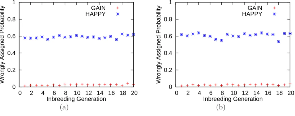
prob-lem. While HAPPY infers the most probable ancestry correctly for more than 80% of the markers, it assigns near 60% of the total probabilities to wrong ancestry choices. The mis-assigned probabilities could hamper further studies. With pedigree structure modeled, GAIN can resolve most ambiguities and assigns only less than 4% of the total probabilities to wrong ancestry.
0 0.2 0.4 0.6 0.8 1
0 2 4 6 8 10 12 14 16 18 20
Wrongly Assigned Probability
Inbreeding Generation GAIN HAPPY
(a)
0 0.2 0.4 0.6 0.8 1
0 2 4 6 8 10 12 14 16 18 20
Wrongly Assigned Probability
Inbreeding Generation GAIN HAPPY
(b)
Figure 2.5: (a) Proportion of probabilities assigned to wrong ancestry by GAIN and HAPPY on a simulated data set with no noise. (b) Proportion of probabilities assigned to wrong ancestry by GAIN and HAPPY on a simulated data set with 1% noise.
2.5.2
Experiments on Real CC data
The data set consists of genotypes of all autosomes from 96 mice of generation G2I5 to
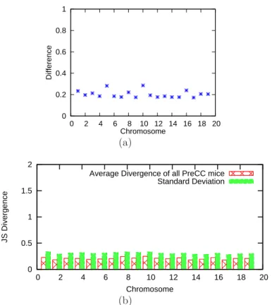
G2I12. The number of SNP markers on each chromosome ranges from 4122 to 35172. Due to the running time constraint of MERLIN, I only compare GAIN with HAPPY which does not consider pedigree structure. Since the true genome ancestry is unknown, I investigate the difference between the results of the two approaches.
dif-data with random error: the results from the two methods differ by 20%. I further mea-sure the difference in probability distributions quantitatively using Jensen-Shannon(JS) Divergence [Lin,1991] which is a smoothed and bounded divergence based on Kullback-Leibler Divergence. The JS Divergence (JSD) between two probability distributions p1 and p2 is defined as:
JSD(p1||p2) =
X
i
p1(i) log2
p1(i) 1
2p1(i) + 1 2p2(i)
+X
i
p2(i) log2
p2(i) 1
2p1(i) + 1 2p2(i)
A low JS Divergence indicates high similarity between p1 and p2. The JS divergence ranges between 0 and 2. Figure 2.6(b) compares the mean and standard deviation of the JS Divergence between HAPPY’s results and ours over all markers and all 96 mice, grouped by chromosomes.
Though I cannot compare the results against the ground truth for real CC data, the source of difference are further investigated. Consider again the CC pedigree in Figure 2.3(a). The initial four founder-mating pairs (F1, F2),(F3, F4), (F5, F6), (F7, F8) cannot serve as ancestry for any genotypes of G2Ik descendants. This is because any
genetic material passed from a founder mating pair is carried by a single haplotype in the G2I0 generation. These four founder pairs are thus invalid ancestry choices if the pedigree structure is considered. As an example to show the improved inference due to incorporating pedigree knowledge, the ancestry of chromosome 7 of a G2I6 mouse inferred by GAIN and HAPPY are shown in Figure 2.7(a) and 2.7(b) respectively. The most probable founder pair inferred by HAPPY agrees with GAIN’s result at most sites. But their actual probabilities are often different. To quantify the extent to which HAPPY assigns positive probabilities to invalid ancestry, at each site l, I aggregate the probabilities of invalid ancestry and plot this “pedigree inconsistency” measure in Figure
0 0.2 0.4 0.6 0.8 1
0 2 4 6 8 10 12 14 16 18 20
Difference
Chromosome
(a)
0 0.5 1 1.5 2
0 2 4 6 8 10 12 14 16 18 20
JS Divergence
Chromosome
Average Divergence of all PreCC mice Standard Deviation
(b)
Figure 2.6: (a) The difference in best ancestry estimated by GAIN and HAPPY (b) The average JS Divergence between results from GAIN and HAPPY on chromosome 1 to 19 of 96 real CC mice.
by the “pedigree inconsistency”. Moreover, the probability distributions of ancestry choices at neighboring sites are not independent. Probabilities assigned to pedigree-inconsistent ancestry can substantially influence the choice of ancestry at neighboring sites. Such “propagated error” is sometimes the main cause of the JS Divergence between HAPPY’s results and ours. As an example, Figure 2.7(d)shows a region in chromosome 1 from another G2I6 mouse where the propagated error is the main cause of divergence. In this region, HAPPY does not assign significant probabilities to invalid ancestry choice, except for a few sites at both ends of this region. But, in the middle part, HAPPY favors ancestry choices that are one recombination away from these invalid ancestry choices.
0 0.2 0.4 0.6 0.8 1
4.0×10⁷ 8.0×10⁷ 1.2×10⁸ 1.6×10⁸
Probability
Location on chromosome (F6,F6) (F2,F6) (F1,F6) (F2,F2) (F1,F8) (a) 0 0.2 0.4 0.6 0.8 1
0.0×100 5.0×10⁷ 1.0×10⁸ 1.5×10⁸
Probability
Location on chromosome (F6,F6) (F2,F6) (F1,F6) (F1,F8) (b) 0 0.2 0.4 0.6 0.8 1
5.0×10⁷ 1.0×10⁸ 1.5×10⁸
Probability
Location on chromosome Pedigree Inconsistency (c) 0 0.2 0.4 0.6 0.8 1
8.0×10⁷ 8.4×10⁷ 8.8×10⁷ 9.2×10⁷
Probability
Location on chromosome Pedigree Inconsistency
Propagated Error
(d)
Figure 2.7: (a) Ancestry inference on chromosome 7 of aG2I6 mouse by GAIN (b)
Ances-try inference on chromosome 7 of the same mouse by HAPPY (c) The pedigree inconsistency in (b), i.e. the aggregated probability assigned to ancestry that violates pedigree knowl-edge. (d) A region in chromosome 1 from another G2I6 mouse where propagated error is
pedigrees can be biased. On the other hand, my method can provide a pedigree consistent inference in comparable running time.
2.5.3
Running Time Performance
For a pedigree containingiinbreeding processes andn′
members not involved in inbreed-ing, the time complexity of GAIN is O(L×n′
×22n′
×28i) where Lis the number of SNP
markers. For any G2Ik animal in CC pedigree, the time complexity remains the same.
The running time does not depend on the error rate of genotype data either. Figure 2.8
shows the running time comparison of GAIN, MERLIN and HAPPY.
1 10 100 1000 10000
0 2 4 6 8 10 12 14 16 18 20
Running Time (s)
Inbreeding Generation MERLIN
GAIN HAPPY
Figure 2.8: Average running time of the three methods on data set containing 6644 markers. The experiment is conducted on an Intel desktop with 2.66Ghz CPU and 8GB memory.
2.6
Discussion
Chapter 3
High Definition Recombination Map
in a Highly Divergent Mouse
Population
3.1
Introduction
[Roberts et al.,2007]. Each of the independently bred lines has equal contributions from all eight founder strains via a funnel breeding scheme (Figure2.3(a)). The eight founder strains are first intercrossed to generate the G1 generation. The G1 progeny are then crossed to create the four-way G2I0 generation. The first eight-way progeny, the G2I1 s are then generated from a G2I0 ×G2I0 cross 1. After this generation, CC strains become inbred by repeated generations of inbreeding through sibling mating. At the top of the funnel, the eight founder strains are arranged in order that is randomized and not repeated across lines. The left four founders contribute to the left half of the funnel and the remaining four contribute to the right half. I also denote the four pairs of founders that are crossed to produce G1 progeny as four quarters of the funnel.
In this study, I focus on theG2I1 generation which has balanced genome contribution from both sides of the funnel pedigree. The breeding pedigree leading toG2I1 generation contains eight observable meioses (Figure3.1). I denote the four at crossingG1 generation as MGM, MGP, P GM, P GP and the four meioses at crossing G2I0 generation as
Mm, Mf, Pm, Pf. Using the genotype data of G2I1 generation, I reconstructed the haplotype at G2I1 generation and inferred all switching points of genome ancestry which correspond to past recombination events in the pedigree. With the design of the breeding scheme, every inferred recombination event can be assigned uniquely to one of the eight meioses. With all recombinations inferred and characterized by gender, meioses and genetic features, this study presents a high definition genome-wide recombination map and associated analysis of its properties.
1
Figure 3.1: The CC funnel pedigree to G2I1 generation. In total there are eight meioses
in the pedigree.
3.2
Materials and Methods
3.2.1
The Genotype Data
• Concordance betweenG2I1mice, founder mice and partially availableG1 genotypes
I kept only 15∼25% of all SNPs on each chromosome in the high-quality group and used only these high-quality SNPs for haplotype reconstruction and recombination infer-ence. The mid-to-low quality SNPs were used later to help refine recombination bound-aries. I also excluded samples2 and chromosomes 3 with exceptionally high discordance
rate in haplotype reconstruction.
3.2.2
Haplotype Reconstruction and Recombination Inference
I utilized the method GAIN to conduct haplotype reconstruction and recombination inference. The method, as described in Chapter 2, is a hidden-Markov-model based method that can model haplotype and recombinations with all pedigree knowledge in-corporated. It has been shown that GAIN can perform analysis in the CC with both high accuracy and scalability with respect to the pedigree size (proportional to number of generations). For the specific G2I1 generation, the model constructed in GAIN is similar to that in an efficient implementation of Lander-Green algorithm (e.g., MERLIN [Abecasis et al.,2001]) because there are no further inbreeding generations. I performed analysis on each funnel independently but jointly on the siblings in the same funnel. This is because siblings can share recombinations and joint analysis can help resolve ambi-guity on recombination locations and haplotype boundaries. Recombinations, however, are not shared across funnels.
For each pair of G2I1 sibling mice, GAIN took the genotypes of the eight founder mice and genotypes of the two sibling mice as input. In addition, it required the funnel order of eight founders. It then inferred the founder ancestry (in probabilities) at each SNP site by building a descendency model at each SNP and evaluating the probabilities of recombining between adjacent SNPs. The founder ancestry at each SNP describes
2
fourteen mouse samples or seven sibling pairs
3
the probability that each pair of founders (e.g., C57BL/6J and CAST/EiJ) are the two founders where the two alleles are inherited from. With pedigree knowledge considered and careful QC steps, GAIN achieved a very high level of confidence in estimating the best ancestry at most sites. More than 98% of the sites in all mice have the best ancestry choice estimated with ≥ 0.99 probability. With the ancestry probability information, I could define the haplotype blocks and recombinations trivially by tracing the most probable founder ancestry along chromosomes. Each recombination event is described by:
• a mid-point where the most probable founder ancestry changes
• proximal and distal boundaries where the probability of the most founder ancestry shrinks to a threshold
• proximal and distal ancestry founders on the recombining chromosome
• the type of meiosis it is associated to
The recombination interval inferred (from proximal to distal boundary) is expected to contain the recombination event with high probability. Note that there are regions where multiple founder ancestries have similar probabilities (due to lack of markers, low geno-typing quality or similar DNA sequence in multiple founders). In such cases, long recom-bination intervals were obtained and the recomrecom-bination events cannot be determined with high resolution.
Upon obtaining the recombination inference results, I further refined them with the mid-to-low-quality SNPs filtered in the QC step. This was done by examining the con-sistency at mid-to-low quality SNPs between founders, each G2I1 mice, and all G2I1 mice assigned the same ancestry. On average, this reduced the recombination intervals inferred by approximately half.
• For any SNP of any G2I1 mouse, the two alleles must come from different halves of the funnel.
• Two siblings cannot inherit different alleles from one quarter funnel at any SNP site.
If the input data contained errors (genotype data or funnel order), GAIN would infer significantly more recombinations in order to satisfy the corresponding constraints. This can be used as an effective indicator to identify and remove:
• Wrongly labeled funnels and mice
• Poorly performing and/or incorrectly mapped SNPs
3.3
Overview of the Recombination Map
Table 3.1: Summary of Identified Recombination Events in G2I1 Mice
Autosomes X chromosome
Meiosis # Type Sex ofG2I1 Non-Shared Shared All Non-Shared Shared All Total
1 M f 3282 - 3282 183 - 183 3465
2 M m 3255 - 3255 150 - 150 3405
3 P f 2871 - 2871 - - - 2871
4 P m 2783 - 2783 - - - 2783
5 MGM f 826 756 1582 35 48 83
m 767 756 1523 35 48 83
all 1593 756 2349 70 48 118 2467
6 MGP f 733 730 1463 - -
-m 768 730 1498 - -
-all 1501 730 2231 - - - 2231
7 PGM f 807 766 1573 174 - 174
m 782 766 1548 - -
-all 1589 766 2355 174 - 174 2529
8 PGP f 740 745 1485 - -
-m 757 745 1502 - -
-all 1497 745 2242 - - - 2242
At a high level, I examined the correctness of the events by checking the ratio between types of events (expected and observed). Firstly, the ratio of shared vs non-shared events is expected to be 1:2 based on Mendel’s Law of Segregation. In the observed data, non-shared events represent 67.3% of events in the MGM, MGP, PGM and PGP meiosis (6,180 out of 9,177 events, the binomial test p-value is 0.17). This is consistently observed in each type of meiosis: MGM, 67.8%; MGP, 67.2%; PGM, 67.5% and PGP, 66.8% (binomial test p-values are 0.25, 0.54, 0.42, 0.93). Secondly, there should not be significant differences in the number of events in same type of meiosis (Mf vs Mm, Pf vs Pm, MGM vs PGM and MGP vs PGP). The ratio of events observed is highly consistent: Mf vs Mm, 1.02; Pf vs Pm, 1.03; MGM vs PGM, 0.975; and MGP vs PGP, 0.999 (binomial test p-values are 0.48, 0.25, 0.39, 0.88). Lastly, the ratio between (M+P) events and (MGM+MGP+PGM+PGP) should be 4:3 (4+34 =.57) 4. I observed 12,191
and 9,177 events, respectively (12191+917712191 =.57, the binomial test p-value is 0.79).
0 200 400 600 800 1000 1200 1400 1600 1800
0 1 2 3 4 5 6 7 8 9
Counts of Unique Events
log10( Recombination Interval Length ) Distribution of Recombination Interval Length
All Non-Shared Shared
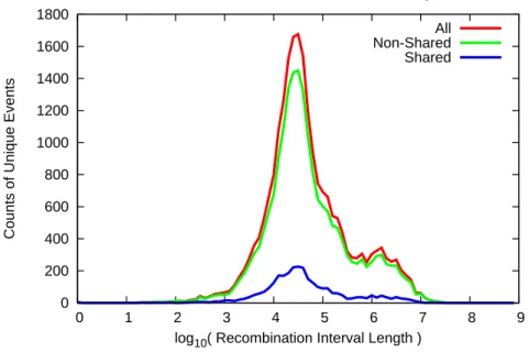
Figure 3.2: Distribution of recombination interval length in log-scale
4
For oneG2I1mouse, we expect to observe four informative independent meiosis. But if we consider
On average, the resolution of recombination events is very high (Figure 3.2). The median size of recombination interval is 35kbp. There are, however, some recombinations that have very large uncertainty intervals (peak in Figure3.2 between 1∼3Mbp). These are mainly due to strain dependent identical-by-descent (IBD) regions or lack of genetic markers in the interval. Based on the 21,993 identified unique recombination events, a recombination density map that can be smoothed at different scales is constructed. When smoothed with windows larger than 500kb, theG2I1 map is remarkably similar to the map recently published but with much lower density of markers [Cox et al.,2009].
3.4
Sex Effect on Recombination
As expected, the total number of recombination events in autosomes is significantly smaller in the male germline than in the female germline (10,127 events and 11, 241 events, respectively; binomial test p-value ≤ 3×10⁻¹⁴
; Table 3.1). This sex difference is also observed in the number of recombination events observed in each individual in bothG1 and G2 meioses. To investigate the possible causes of this difference, the effect of the Prdm9 genotype on the size of the autosomal map was determined. One of the eight founder strains of the CC, CAST/EiJ, carries the Prdm9a allele, four strains
(A/J, C57BL/6J, 129S1/SvImJ and NZO/HILtJ) carry the Prdm9b allele, two strains
(NOD/ShiLtJ and WSB/EiJ) carry the Prdm9c allele and the PWK/PhJ strain carries
the Prdm9d allele. There is a significant expansion of the female map length and a
reduction of the male map length in carriers of the Prdm9a allele (1,450 cM and 1,195 cM, respectively). There is also a significant contraction of the female map length and an expansion of the male map length in carriers of thePrdm9dallele (1,300 cM and 1,325
cM, respectively). Finally, carriers of bothPrdm9b and Prdm9c alleles have similar ratio
Figure 3.3: Recombination map length of autosomes byPrdm9 allele and gender
the distal peak is both higher and sharper than in singles and the proximal peak is lower and much wider. This pattern suggests that recombination may progress temporally from the telomere to centromere in males.
0 0.5 1 1.5 2 2.5 3 3.5
0 0.2 0.4 0.6 0.8 1
Kernel density estimate of recombination
Relative distance along chromosome
(a) female meioses
0 0.5 1 1.5 2 2.5 3 3.5
0 0.2 0.4 0.6 0.8 1
Kernel density estimate of recombination
Relative distance along chromosome
(b) male meioses
Figure 3.4: Distribution of recombination events along the autosomes in female and male meioses. The x-axis corresponds to the relative position in all autosomes. The y-axis indicates the kernel density estimates of recombinations in each type of meiosis.
3.5
Cold Regions
Regions with low levels of recombination have been reported previously [Smagulovaet al.,
0 0.5 1 1.5 2 2.5 3 3.5
0 0.2 0.4 0.6 0.8 1
Kernel density estimate of recombination
Relative distance along chromosome
(a) female meioses, single recombinant
0 0.5 1 1.5 2 2.5 3 3.5
0 0.2 0.4 0.6 0.8 1
Kernel density estimate of recombination
Relative distance along chromosome
(b) female meioses, double recombinants
0 0.5 1 1.5 2 2.5 3 3.5
0 0.2 0.4 0.6 0.8 1
Kernel density estimate of recombination
Relative distance along chromosome
(c) male meioses, single recombinant
0 0.5 1 1.5 2 2.5 3 3.5
0 0.2 0.4 0.6 0.8 1
Kernel density estimate of recombination
Relative distance along chromosome
(d) male meioses, double recombinants
reduce the size of many candidate regions of interest is undermined by an apparent lack of recombination. However, we know very little about the size, distribution, genomic fea-tures and evolutionary stability of such regions. Thus identification and characterization of such cold regions may provide important information on the distribution of genetic variation and the level of linkage disequilibrium in the mammalian genome, the accuracy of imputation of genetic variants and may provide new models to study the molecular and cellular mechanisms of meiotic recombination.
3.5.1
Identification of Cold Regions in the
G
2
I
1Population
Cold regions are defined as long (>500 kb) continuous genomic intervals that are markedly depleted of recombination events in the G2I1 population. Given the total number of recombination events in my experiment (∼22,000) I set up this 500 kb threshold in the initial identification of cold regions to reduce the number of false positives (i.e., on average I expect 8.7 recombination events per Mb).
3.5.2
External Validation of Cold Regions
To determine whether the results in theG2I1 population are replicable in other popula-tions, I estimated the recombination rate in these regions in the heterogeneous stock used to construct the most recent linkage map of the mouse [Cox et al., 2009]. On average, there is a four-fold reduction in recombination density in cold regions (0.14 cM/Mb ver-sus the expected 0.5 cM/Mb that is observed genome wide). In fact, 57 of the 59 regions are below the genome wide average and for 16 regions the recombination density in the Cox map is zero (Table 3.2). The extent of validation is striking given the differences in genetic background (only five of the 16 strains are shared between these two studies and the non shared strains include three wild derived strains representing two subspecies that are rare or absent in the genetic makeup of the strains in the Cox study), marker density and approach to estimate recombination distances between these two populations.
Recently, several maps of recombination initiation sites in the mouse have been pub-lished [Smagulova et al., 2011; Brick et al., 2012]. These studies identified regions with significant enrichment of double strand breaks (DSB) in the male germline of mice of dif-ferent genetic backgrounds. Smagulova et al. [2011] identified 21 recombination deserts larger than 3 Mb, but noted that the inability of identifying hotspots in some of these re-gions may be due to sequencing gaps or highly repetitive DNA. Eleven of the cold rere-gions identified in the G2I1 population overlap with those described previously in Smagulova et al. [2011]. This level of concordance is even more remarkable once one considers that one of the Smagulova desserts was eliminated from my analysis because of complete lack of sequence5 and the fact that nine additional regions that fail to make the cut in my list