5323.pdf

(1)

SCHEDULING MIXED-CRITICALITY

REAL-TIME SYSTEMS

Haohan Li

A dissertation submitted to the faculty of the University of North Carolina at Chapel Hill in partial fulfillment of the requirements for the degree of Doctor of Philosophy in the Department of Computer Science.

Chapel Hill 2013

Approved by:

Sanjoy K. Baruah

James H. Anderson Kevin Jeffay

Montek Singh

(2)

(3)

ABSTRACT

HAOHAN LI: Scheduling Mixed-Criticality Real-Time Systems (Under the direction of Dr. Sanjoy K. Baruah)

This dissertation addresses the following question to the design of scheduling policies and resource allocation mechanisms in contemporary embedded systems that are implemented on integrated computing platforms: in a multitasking system where it is hard to estimate a task’s worst-case execution time, how do we assign task priorities so that 1) the safety-critical tasks are asserted to be completed within a specified length of time, and 2) the non-critical tasks are also guaranteed to be completed within a predictable length of time if no task is actually consuming time at the worst case?

This dissertation tries to answer this question based on the mixed-criticality real-time system model, which defines multiple worst-case execution scenarios, and demands a scheduling policy to provide provable timing guarantees to each level of critical tasks with respect to each type of scenario. Two scheduling algorithms are proposed to serve this model. The OCBP algorithm is aimed at discrete one-shot tasks with an arbitrary number of criticality levels. The EDF-VD algorithm is aimed at recurrent tasks with two criticality levels (safety-critical and non-critical). Both algorithms are proved to optimally minimize the percentage of computational resource waste within two criticality levels. More in-depth investigations to the relationship among the computational resource requirement of different criticality levels are also provided for both algorithms.

(4)

(5)

ACKNOWLEDGEMENTS

I have always been feeling lucky when I pursue the doctoral degree at The University of North Carolina at Chapel Hill, because I have received too much help and support to repay. The first and the most important of all, the best part of my graduate student life is to have Sanjoy Baruah as my advisor. He shows me how attractive the computer science research is, how kind a teacher can be, and how wonderful an academic life will be. It wouldn’t be possible for me to become who I am without him, and it is my dream to become who he is.

I would like to express my sincerest appreciation to my committee members: Jim Anderson, Kevin Jeffay, Montek Singh, and Leen Stougie, for the time and energy they spend on my dissertation. It is my great fortune to receive guidance and advices from them during my work. I am also very grateful to my co-authors: Vincenzo Bonifaci, Gianlorenzo D’Angelo, Alberto Marchetti-Spaccamela, Nicole Megow, Suzanne Van Der Ster, Bipasa Chattopadhyay, and Insik Shin. It is my honor and my pleasure to work with so many great minds on numerous interesting problems.

I want to thank all my friends in the real-time systems group, from whom I learn a lot: Cong Liu, Mac Mollison, Glenn Elliott, Zhishan Guo, Jeremy Erickson, Bryan Ward, Alex Mills, Andrea Bastoni, Hennadiy Leontyev and Bj¨orn Brandenburg. The delightful memory in this great group will never fade away.

I am extremely proud to spend five years in The Department of Computer Science at UNC. I am grateful to the department for awarding me the Computer Science Alumni Fellowship that supports my dissertation writing. Also, I appreciate the infinite help from all the faculty members and staffs. Especially, I would like to say thanks to Jodie Turnbull for her splendid service and unreserved help during my study and job hunting.

I wish to say “thank you” to my parents, for their constant and unconditional love.

(6)

(7)

LIST OF TABLES

1.1 DO-178B Standard . . . 5

(10)

LIST OF FIGURES

4.1 EDF-VD: The preprocessing phase. . . 48

(11)

LIST OF ABBREVIATIONS

CA Certification Authority CM Criticality-Monotonic EDF Earliest-Deadline-First

EDF-VD Earliest-Deadline-First with Virtual Deadlines FAA Federal Aviation Administration

LCM Least Common Multiple

LHS Left-Hand Side

MC Mixed-Criticality

NP Non-deterministic Polynomial-time OCBP Own-Criticality-Based-Priority

RTCA Radio Technical Commission for Aeronautics SWaP Size, Weight and Power

UAV Unmanned Aerial Vehicle WCET Worst-Case Execution Time WCR Worst-Case Reservation

(12)

CHAPTER 1

Introduction

Traditional real-time scheduling theory faces challenges in modern computation-intensive and time-sensitive cyber-physical embedded systems. Nowadays, real-time embedded comput-ing systems are widely used in safety-critical environments such as avionics and automobiles. There are two conflicting trends in the development of these systems. One is that the safety assurance requirements are increasingly emphasized. Some critical real-time tasks must never fail to meet their deadlines, even under extremely harsh circumstances. The other is that more functionalities are implemented on integrated platforms due to size, weight and power (SWaP) constraints. Therefore, many non-critical real-time tasks will share and compete for the computational resources with critical tasks. Unfortunately, traditional real-time scheduling theory cannot provide a balance between these two requirements. The existing techniques have to reserve unreasonably large amounts of computational resources to ensure that every real-time task performs correctly under harsh circumstances — even the non-critical ones. This inefficiency makes it desirable that the assumptions, abstractions and objectives in traditional real-time scheduling theory be reconsidered, such that these safety-critical systems will sacrifice neither reliability nor efficiency.

1.1 Overview of Real-Time Systems

(13)

actions at the required time”, which is an additional main objective in real-time systems.

Real-time systems are defined as systems that provide temporal correctness. In real-time systems, the temporal predictability, which is often in the form of guaranteeing every task’s response within strict deadlines, is as important as the performance (how fast an individual task can complete) or the throughput (how many tasks can be completed over a long period of time).

In real-time scheduling theory research, the scheduling algorithms that switch tasks and allocate resources in real-time systems are studied. These algorithms are constructed based on real-time task models. These models will be introduced in Section 1.3. These models extract the essential information of the temporal behaviors of the tasks in a real-time system. The scheduling algorithms must predictably assure a priori that all tasks are completed by their deadlines, assuming that the tasks follow the specifications in the workload model. Because these guarantees must be analytically proved before the actual execution of the system, there are usually two types of algorithms on scheduling:

Scheduling policies, sometimes calledschedulers, are the algorithms that control the run-time schedule. The scheduling policies will be executed along with real-time tasks, and make scheduling decisions based on the time and/or the temporal behavior of real-time tasks. Scheduling policies are generally required to be simple and fast because they compete with real-time tasks and occupies computational resources.

Schedulability tests are the algorithms that check before run-time if the deadlines are guaranteed to be met. Schedulability tests can be complicated and time-consuming if they can bring in better run-time performance and computational resource efficiency. It is non-trivial to design schedulability tests, especially for real-time tasks with a large variance of run-time behaviors because the tests must guarantee that no deadline is missed in all possible system runs.

This dissertation focuses on a new real-time task model, the mixed-criticality task model. Section 1.3 will describe the traditional model, the new model, and their differences. The following chapters in this dissertation will introduce several scheduling algorithms aimed at

(14)

the mixed-criticality system model, while Section 1.5 gives an overview of all these scheduling algorithms.

1.2 Motivation

The research of scheduling mixed-criticality systems starts from abstracting a realistic problem — the certification requirement. Many safety-critical embedded systems must pass certain safety certifications. In the certification processes, the certification authorities, such as Federal Aviation Administration (FAA), will verify the safety standards within the system, including the real-time constraints of the safety-critical tasks. It is important to note that the certification authorities tend to be very conservative in the certification. They require that the correctness be demonstrated under extremely rigorous and pessimistic assumptions, which are very unlikely to occur in reality.

(15)

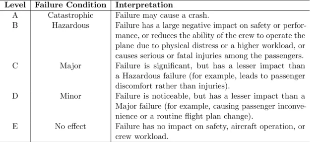
Knowing the shortcomings of the traditional models, how do we abstract a certifiable real-time system, and what kind of scheduling policies do we seek then? The key idea is to observe that in many applications, the consequence of a deadline miss varies among tasks. For example, in the RTCA DO-178B avionics software standard, as listed in Table 1.1, the tasks are divided into five assurance levels, from level A to level E. In the standard, a failure of a level-A task will have catastrophic results (e.g. causing a crash), while a failure of a level-E task will have no influence on flight safety. Under these circumstances, it is reasonable not to presuppose an objective that all low-criticality deadlines are always met. Therefore, the mixed-criticality real-time system model is proposed by Vestal (Vestal, 2007) on the basis of a new assumption that only high-criticality deadlines are guaranteed to be met if high WCET estimations are used, and all deadlines are guaranteed to be met if low

WCET estimations are used. Under this new assumption, only high-criticality tasks will reserve a large amount of time while several thresholds of possible execution time are also defined. Low-criticality tasks will be executed only if the execution of high-criticality tasks execute shorter than a certain threshold. Now when the certification authorities assume high WCET estimations, the high-criticality tasks will perform correctly; but the system is still able to perform many real-time functionalities if these high-criticality tasks execute normally.

1.3 Models for Real-Time Systems and Mixed-Criticality

Systems

In this section, we introduce the models used in real-time systems and mixed-criticality real-time systems. The models in classic real-time systems will be introduced briefly, while detailed examples and formalized definitions (Vestal, 2007; Baruah et al., 2010b) will be given pertaining to models in mixed-criticality real-time systems.

1.3.1 Real-time Jobs and Recurrent Tasks

There are many real-time task models in classic real-time systems, although the principle remains the same: a piece of code becomes available for execution at a time moment in the

(16)

Level Failure Condition Interpretation

A Catastrophic Failure may cause a crash.

B Hazardous Failure has a large negative impact on safety or perfor-mance, or reduces the ability of the crew to operate the plane due to physical distress or a higher workload, or causes serious or fatal injuries among the passengers. C Major Failure is significant, but has a lesser impact than

a Hazardous failure (for example, leads to passenger discomfort rather than injuries).

D Minor Failure is noticeable, but has a lesser impact than a Major failure (for example, causing passenger inconve-nience or a routine flight plan change).

E No effect Failure has no impact on safety, aircraft operation, or crew workload.

Table 1.1: DO-178B is a software development process standard,Software Considerations in Airborne Systems and Equipment Certification, published by RTCA, Inc. The United States Federal Aviation Administration (FAA) accepts the use of DO-178B as a means of certifying software in avionics applications. RTCA DO-178B assigns criticality levels to tasks categorized by effects on commercial aircraft.

system, takes a certain amount of time to finish its execution, and is required to finish by a given time moment. The variety of the task models is derived from the definition of the manner which the available time, execution time and deadline follow. In this dissertation, we only consider two kind of real-time task models:

Real-time jobs. This is the simplest task model. In this model, a job, representing a piece of code, is available at a specified time, and is required to be finished by another specified time. These two time instants are known asthe release time andthe deadline. They can be expressed in absolute (“wall-clock”) time, or relative time with respect to a given time instant that is defined as time 0 (usually this time instant is when the whole system starts working, or the first release time in the system). In either case, neither of the two time instants will change as time goes on.

Real-time sporadic tasks. This is the most commonrecurrent task model. A recurrent

(17)

to be (repeatedly) executed. The task will have a parameter, itsrelative deadline, so that when a job is released, it will have its deadline as its release time plus the relative deadline. The jobs cannot be released infinitely frequently — aminimum inter-arrival time between any two consecutive job releases is specified, and defined as the task’s

period. In a sporadic task system, it is not possible to know the exact release times of the jobs in this system. However, in any time interval that is no longer than a task’s period, there can be at most one job release.

In both task models, it is very important to pre-evaluate the amount of time that a job requires, in order to assure that no job will miss its deadline. This amount of time is represented by the job’s worst-case execution time (WCET). In this dissertation, we will not discuss the techniques that are used to evaluate a job’s execution time. We only assume that this parameter is known for every job, and a job is guaranteed to be completed if it has been accumulatively executing for its worst-case execution time.

As a summary, a real-time job is specified by three parameters: its release time, its deadline, and its worst-case execution time; a real-time sporadic task is also specified by three parameters: its period, its relative deadline, and its worst-case execution time. A real-time sporadic task can generate infinitely many real-time jobs.

Now we can define the system using the previously described models. We will consider the systems that consist of only real-time jobs, or only real-time tasks. To fully describe the properties of a system, we need more terms, which are provided below.

In this dissertation, onlypreemptive systems are considered. Preemptive means that at any time, the scheduling policy can suspend the current executing job, and choose another job (that can be executed) to execute. Though preemption causes context and state saving and costs additional time in reality, we assume in this dissertation that any additional time cost has been bounded by the worst-case execution time. Therefore, in our scheduling polices, we will not analytically limit the number of preemptions (pragmatic limitations may be applied, however).

All our previous statements assume hard real-time systems, which means that deadlines can never be missed, or the scheduling policy will be determined as faulty. Soft real-time

(18)

systems, which tolerate deadline miss in certain pre-defined manners, will not be discussed in this dissertation.

The demand of computational resource is an important property of a system. Load

can be used to describe both real-time jobs and real-time recurrent tasks. It denotes the

maximum fraction of processor time demand of a system over any time interval. Utilization

is used only to describe real-time recurrent tasks. It denotes theoverall fraction of processor time demand of a system. Here thetime demand over a given interval means the summation of the WCETs of the jobs that are released in this interval and is required do be finished in this interval. The formal definitions can be found in Subsection 1.3.3 and 1.3.4.

1.3.2 Overview of Mixed-Criticality Systems

In this subsection, we introduce the detailed mixed-criticality system model by considering first an example from the domain of unmanned aerial vehicles (UAVs), used for defense reconnaissance and surveillance. The functionalities on board such UAVs may be classified into two levels of criticality:

Level 1: mission-critical functionalities, concerning reconnaissance and surveillance objectives, like capturing images from the ground, transmitting these images to a base station, etc.

Level 2: flight-critical functionalities: to be performed by the aircraft to ensure its safe operation.

(19)

This difference in correctness criteria may be expressed by differentWorst-Case Execution Times (WCET) estimates for the execution of a piece of real-time code. In fact, the CA and the system designers (and other parties responsible for validating the mission-critical functionalities) will each have their own tools, rules, etc., for estimating WCET; the value so obtained by the CA is likely to be larger (more pessimistic) than the one obtained by the system designer. We illustrate via a (contrived) example.

Example 1.1. Consider a system comprised of two jobs: J1 is flight-critical whileJ2 has lower mission-critical criticality. Both jobs arrive at time-instant 0, and have their deadlines at time-instant 10. Fori∈ {1,2}, letCi(1) denote the WCET estimate of jobJi as made by the system designer, and Ci(2) the WCET estimate of jobJi as made by the CA.

As we have stated above, WCET values determined by the CA tend to be larger than those determined by the system designer. Suppose that C1(1) = 3, C1(2) = 5 and C2(1) =C2(2) = 6. Consider the schedule that first executes J1 and thenJ2.

The CA responsible for safety-critical certification would determine thatJ1 completes latest by time-instant 5 and meets its deadline. (Note that if the execution time ofJ1 is 5 then in the worst case it is not possible to completeJ2 by its deadline; however, this CA is not interested inJ2; hence the system passes certification.)

The system designers (and other parties responsible for validating the correctness of the mission-critical functionalities) determine that J1 completes latest by time-instant 3, andJ2 by time-instant 9. Since both jobs complete by their deadlines, the system is determined to be correct by its designers.

We thus see that the system is deemed as being correct by both the CA and the designers, despite the fact that the sum of the WCET’s of the jobs at their own criticality levels (6 and 5) exceeds the length of the time window over which they are to execute.

Current practice in safety-critical embedded systems design for certifiability is centered around the technique of “space-time partitioning”. Loosely speaking, space partitioning

means that each application is granted exclusive access to some of the physical resources on board the platform, and time partitioning means that the time-line is divided into slots with each slot being granted exclusively to some (pre-specified) application. Interactions

(20)

among the partitioned applications may only occur through a severely limited collection of carefully-designed library routines. This is one of severalreservation-based approaches, in which a certain amount of the capacity of the shared platform is reserved for each application, that have been considered for designing certifiable mixed-criticality systems. It is known that reservation-based approaches tend to be pessimistic (in the sense of under-utilizing platform resource); for instance, a reservation-based approach to the example above would require that 5 units of execution be reserved for job J1, and 6 units for job J2, over the interval [0,10).

1.3.3 Mixed-Criticality Jobs

Although the example that we considered in Section 1.3.2 is characterized by just two criticality levels, systems may in general have more criticality levels defined. (For instance, the RTCA DO178-B standard in Table 1.1, widely used in the aviation industry, specifies five different criticality levels, with the system designer expected to assign one of these criticality levels to each job. The ISO 26262 standard, used in the automotive domain, specifies four criticality levels, known in the standard as “safety integrity levels” or SILs.)

Accordingly, the formal model that we use allows for the specification of arbitrarily many criticality levels. LetL∈N+ denote the number of distinct criticality levels in the mixed-criticality system being modeled.

Definition 1.1. Amixed-criticality job in the mixed-criticality system is characterized by a 4-tuple of parameters: Jj = (aj, dj, χj, Cj), where

aj ∈Q+ is the release time;

dj ∈Q+ is the deadline, dj ≥aj;

χj ∈N+ is the criticality of the job;1

Cj ∈QL+ is a vector, the k-th coordinate of which specifies the worst-case execution time (WCET) estimate of job Jj at criticality levelk. In a job-specification we will usually represent it by (Cj(1), . . . , Cj(L)).

1_{If there are only two criticality levels in the system, we can also use level}

loand levelhiinstead of level

(21)

We will, for the most part, assume that Cj(k) is monotonically non-decreasing with increasingk. This is a reasonable assumption: theseCj(k) values representupper bounds, at different degrees of confidence, on the WCET of the job. Larger values ofk correspond to greater degrees of confidence, and are therefore likely to be larger. At any moment, we call a jobavailable if its release time has passed and the job has not yet completed execution.

An instance I of the MC-schedulability problem consists of a set of n jobs. In this dissertation we assume that there is only one machine (processor) to execute the jobs. However, we have some results on multiprocessor, which is briefly introduced in Section 6.2. We assume that this processor is preemptive: executing jobs may have their execution interrupted at any instant in time and resumed later, with no additional cost or penalty.

To define MC-schedulability we define the notion of a scenario.

Definition 1.2. Each job Jj requires an amount of execution timecj within itstime

win-dow[aj, dj]. The value ofcj is not known from the specification of Jj, but is only discovered by actually executing the job until itsignals that it has completed execution. This charac-terizes the uncertainty of the problem. We call a collection of realized values (c1, c2, . . . , cn) a scenarioof instanceI.

Definition 1.3. The criticality level, or simply criticality, of a scenario (c1, c2, . . . , cn) of I is the smallest integer ksuch that cj ≤Cj(k) for allj= 1, . . . , n. (If there is no such k, we define that scenario to be erroneous.)

Definition 1.4. A schedule for a scenario (c1, . . . , cn) of criticality k is feasible if every job Jj withχj ≥kreceives execution time cj during its time window [aj, dj].

A clairvoyant scheduling policy knows the scenario of I, i.e., (c1, . . . , cn), prior to determining a schedule for I.

Definition 1.5. An instanceI isclairvoyantly-schedulableif for each non-erroneous scenario of I there exists a feasible schedule.

In contrast to clairvoyant scheduling policies, an on-linescheduling policy discovers the value ofcj only by executing Jj until it signals completion. In particular, the criticality level of the scenario becomes known only by executing jobs. At each time instant, scheduling decisions can be based only on the partial information revealed thus far.

(22)

Definition 1.6. An on-line scheduling policy iscorrectfor instanceI if for any non-erroneous scenario of instanceI the policy generates a feasible schedule.

Definition 1.7. An instanceI isMC-schedulable if there exists a correct on-line scheduling policy for instance I.

It is very obvious to see that a MC-schedulable instance I must be also clairvoyant-schedulable because otherwise there will be scenarios that do not have a feasible schedule.

The MC-schedulability problem is to determine whether a given instance I is MC-schedulable or not.

Example 1.2. Consider an instanceI of adual-criticality system: a system withL= 2. I

is comprised of 2 jobs: jobJ1 has criticality level 1 (which is the lower criticality level), and the other job has the higher criticality level 2.

J1 = (0,2,1,(1,1))

J2 = (0,3,2,(1,3))

For this example instance, any scenario in whichc1andc2, are no larger than 1, has criticality 1; while any scenario not of criticality 1 in which c1 and c2 are no larger than 1, and 3, respectively, has criticality 2. All remaining scenarios are, by definition, erroneous. It is easy to verify that this instance is clairvoyantly-schedulable.

Policy S0, described below, is an example of an on-line scheduling policy for instance I:

S0: Execute J2 over [0,1]. If J2 has no remaining execution (i.e., c2 is revealed to be no greater than 1), then continue with schedulingJ1over (1,2]; else continue by completely scheduling J2.

It is easy to see that policy S0 is correct for instanceI. However, S0 is not correct if we modify the deadline ofJ1 obtaining the following instance I0:

J1 = (0,1,1,(1,1))

J2 = (0,3,2,(1,3))

(23)

It is easy to see that I0 is clairvoyantly schedulable but not MC-schedulable. Any on-line scheduling policy that starts with executing J1 will cause J2 to miss its deadline if c2 is revealed to be 3; any on-line scheduling policy that starts with executing J2 will causeJ1 to miss its deadline if c2 is revealed to be no greater than 1.

Speedup factors are a useful conceptual characterization of the effectiveness of a schedul-ing policy, and may provide valuable insight into the policy’s properties.

Definition 1.8. The speedup factor xfor a scheduling policy A is defined as the minimum factor by which the speed of the processor would need to be increased such that all instances/systems that are schedulable according to a clairvoyant scheduling policy on a processor become schedulable under the policy A.

A speedup factorxof the scheduling policyAis calledexactif there exists an instance/sys-tem that is schedulable on processor(s) of speed 1 by an optimal (possibly clairvoyant) scheduling policy but is not schedulable byA on any processor(s) of speed lower thanx.

A scheduling policyA with speedup factorx is called optimal with respect to speedup factors if there exists an instance/system that is schedulable on processor(s) of speed 1 by the optimal (andclairvoyant) scheduling policy but is not schedulable by any on-line

scheduling policies on any processor(s) of speed lower than x.

Loads are also a useful conceptual characterization of the effectiveness of a scheduling policy, and provide more in-depth investigation to the relationship among the computational resource requirement of different criticality levels. Analogous to the load concept in traditional real-time task models, we find it convenient to define loads of a MC instanceI in different criticality levels:

Definition 1.9. Given a MC instanceI, the load of I in criticality level k(1≤k≤L) is defined as the maximum ratio between the sum of criticality level kWCETs in any time interval and the length of this time interval. It can be written formally as:

`k= max 0≤t1<t2

X

Ji :χi≥k∧t1≤ai∧di≤t2

Ci(k)

t2−t1

(1.1)

(24)

Informally, `k is the largest proportion of processor occupation that the system expects to have to deal with during run-time while executing instanceI in a behavior of criticality level k. Clearly, it is necessary (albeit not sufficient) that all`k be no larger than the speed of the processor on whichI is to be executed.

All `k for a MC instanceI with njobs can be determined in time that is polynomial in

n. To see this, we observe that only such values oft1 and t2 need be considered where t1 is equal to someai andt2 is equal to somedi. There are no more thann2 possible such [t1, t2) intervals, and computing the sum of the WCET estimates over each interval takes O(n) time. Thus even with the brute-force method, we can compute both loads inO(n3) time.

1.3.4 Mixed-Criticality Recurrent Tasks

Definition 1.10. A mixed-criticality sporadic task in the mixed-criticality system is char-acterized by a 4-tuple of parameters: τj = (χj, Cj, Tj, Dj), where

χj ∈N+ is the criticality of the task;

Cj ∈QL+ is a vector, the k-th coordinate of which specifies the worst-case execution time (WCET) estimate at criticality levelk;

Tj ∈Q+ is the period;

Dj ∈Q+ is the relative deadline.

Task τj generates a potentially infinite sequence of jobs, with successive jobs being released at least Tj time units apart. Each such job has a deadline that is Dj time units after its release. The criticality of each such job isχj, and it has the WCET estimation vector as

Cj = (Cj(1), . . . , Cj(L)).

A MC sporadic task set is specified by specifying a finite number of such sporadic tasks. As with traditional (non-MC) systems, such a MC sporadic task set can potentially generate infinitely many different MC instances (collections of jobs), each instance being obtained by taking the union of one sequence of jobs generated by each sporadic task.

(25)

restriction is placed on the relation between periods and deadlines. Implicit-deadline sporadic tasks are a special case of arbitrary-deadline sporadic tasks.

The definition of loads extends in the obvious manner to systems of sporadic tasks: The load `k of sporadic task system τ is defined to be the largest value that `k can have, for any instanceI generated byτ. However, the computation of loads in sporadic systems is harder than in in job sets (ususally impossible in polynomial time). We will introduce the computation of loads in sporadic systems later.

Utilization is another conceptual characterization of a sporadic task system.

Definition 1.11. Given a MC sporadic task setτ, the utilization ofτ in criticality levelk

(1≤k≤L) is defined as

Uk=

X

τj:χj≥k

Cj(k)

Tj

. (1.2)

Moreover, the utilization at levelk of jobs that are of criticality leveliis defined as

Uk(i) =

X

τj:χj=i

Cj(k)

Tj

. (1.3)

Utilizations are defined over all sporadic task sets. but it is the most useful for implicit-deadline sporadic task set, or in soft-real-time systems. In this dissertation, we only use utilizations to evaluate scheduling policies in Chapter 4. It is easy to see that in a MC implicit-deadline sporadic task set, `k = Uk for all 1≤k ≤L. The reason is that in any given time interval [t1, t2), the time demand can not exceed Uk(t2−t1). Therefore Uk≥`k must hold. The “equal” can be reached at the LCM of all periods.

1.4 Thesis Statement

The central thesis explored in our research is thatefficient resource allocation in systems that are subject to multiple different correctness criteria requires the development of new

approaches for resource-allocation and scheduling. This dissertation describes our efforts to date towards developing such approaches. Therefore, the thesis statement is as follows:

(26)

New methods can be discovered to schedule real-time systems with multiple criticalities. The methods can supply multiple temporal predictability assertions with respect to multiple WCET specifications. The assertions can be defined and measured through a formalized description. The methods can be efficiently implemented with acceptable computational complexities.

1.5 Contributions

(27)

The more general and popular abstraction to real-time tasks in real-time system research is the sporadic task model, where the jobs are released recurrently with minimum time gaps. Thus the second question to the mixed-criticality system is whether the mixed-criticality sporadic tasks can be efficiently scheduled. In order to answer this question, the classic Earliest-Deadline-First (EDF) algorithm is specialized to support mixed-criticality systems. In the traditional real-time scheduling, EDF is proved to be an optimal exact algorithm on preemptive uniprocessor platform. Its philosophy of favoring urgent jobs, in the form of always choosing the job with the earliest deadline to execute, provably maximizes the use of processor capacity in the traditional real-time systems. Yet in order to promote high-criticality tasks in mixed-criticality systems as mentioned above, these tasks will be given earlier virtual deadlines to reflect their importance over low-criticality tasks. This modified EDF algorithm (named EDF-VD, where VD stands for virtual deadlines) has a speedup factor of 4/3 for mixed-criticality sporadic systems with two criticality levels and implicit deadlines, while this factor is also shown as minimal for the mixed-criticality implicit-deadline sporadic task systems. This modified EDF algorithm is also extended to mixed-criticality arbitrary-deadline sporadic task sets, and is proved to have a speedup factor as 1.83.

Besides these two main contributions, other research results will also be mentioned in Chapter 6. The OCBP algorithm is generalized according to the sporadic task model. The challenge is that a sporadic task can release infinite jobs at indefinite time instants. An on-line priority adjustment technique is proposed to deal with unanticipated job releases while preserving the speedup factor. It uses a priority list computed by the OCBP algorithm for a longest and densest possible job release sequence, and recomputes the priority list to dynamically secure the correctness of the ongoing schedule at the instant when a new job releases. The EDF-VD algorithm is extended to the main two categories in the multiprocessor scheduling theory: the global multiprocessor scheduling (tasks and jobs can migrate among processors) and thepartitioned multiprocessor scheduling (tasks are assigned to dedicated processors). An initial effort is made on analyzing the mixed-criticality multiprocessors scheduling problem. Both based-on the EDF-VD algorithm, the global scheduling policy adjusts the deadlines of high-criticality tasks so that the system is schedulable when the

(28)

(29)

CHAPTER 2

Prior Work

In this chapter, we briefly review important research results related to mixed-criticality scheduling. In Section 2.1, important results in traditional real-time scheduling theory that are helpful to mixed-criticality scheduling are introduced, including the optimal scheduling policy EDF, and the relationship between loads, utilizations and schedulability. In Section 2.2, research results on the mixed-criticality model in this dissertation and on other similar real-time task models are presented.

2.1 Real-Time Scheduling Theory

In this section, we first introduce the EDF scheduling policy, then show its optimality and schedulability conditions.

Definition 2.1. Earliest-deadline-first (EDF) scheduling policy always selects the job with the earliest deadline in all available jobs to execute at any time moment.

Theorem 2.1. (Liu and Layland, 1973; Horn, 1974)If a real-time job instance or sporadic task set is schedulable on a uniprocessor by any scheduling policy, it is also schedulable by

EDF.

(30)

the moment and order of its execution. Therefore, this scheduling policy is not optimal any more when applied to mixed-criticality task models, because if the execution order of the jobs is changed, the time demand may differ — low-criticality jobs may be ignored after the high-criticality behavior is revealed.

Example 2.1. Consider an dual-criticality job instance I that consists of two jobsJ1 and

J2. As we denote a job asJj = (aj, dj, χj, Cj), the two jobs are represented as

J1 = (0,4,2,(2,4))

J2 = (1,3,1,(1,1)).

Now if we consider the EDF scheduling policy inlow-criticality behavior of this instance, the run-time behavior will be: (1) at time instant 0, start executingJ1; (2) at time instant 1, suspend J1 and start executing J2, becauseJ2 is available to execute and has the earliest deadline in all available jobs (J1 and J2); (3) at time instant 2, J2 is completed so start executing J2 again; (4) at time instant 3, complete J1 (because it is the low-criticality behavior) which meets its deadline.

It is important to note that even if we do not know the parameters (including release times, deadlines and WCETs) of all or any jobs, the scheduling decisions made by EDF scheduling policy will remain the same. Like in the example, assuming that J2’s release time isn’t known beforehand, at time instant 1 whenJ2 is actually released, EDF scheduling policy will pick J2 for execution.

However, if we consider the high-criticality behavior of this instance which includes a criticality change, EDF scheduling policy isn’t correct (thus non-optimal) any more. If we simulate the run-time behavior again, it will be: (1) at time instant 0, start executing

J1; (2) at time instant 1, suspend J1 and start executing J2; (3) at time instant 2, J2 is completed so start executing J2 again; (4) at time instant 5, completeJ1 (because it is the high-criticality behavior) which misses its deadline.

(31)

and discardJ2, becauseJ2 can miss its deadline validly if J1 uses more than C1(1) = 2 time units.

Theorem 2.2. (Baruah et al., 1990) A real-time job instance or sporadic task set is schedulable by EDF if and only if its load is no greater than 1.

The original theorem in (Baruah et al., 1990) is presented in the form of DBF (demand bound function). Basically, it states the fact that as long as the time demand does not exceed the processor capacity in any time interval (or briefly “processor is not over-utilized”), the system is schedulable by EDF.

Though it appears that the calculation of the load of a system is a good method to perform a schedulability test, the following two theorems show that the calculation for sporadic task sets is computationally expensive.

Theorem 2.3. (Baruah et al., 1990; Eisenbrand and Rothvoß, 2010)The problem of deciding whether a real-time arbitrary-deadline sporadic task set is schedulable is coNP-hard.

Theorem 2.4. (Baruah et al., 1990) The load of a real-time arbitrary-deadline sporadic task set can be computed in pseudo-polynomial time if the utilization of the task set is less

than 1.

Theorem 2.3 and 2.4 indicate that there is no polynomial-time schedulability test for arbitrary-deadline sporadic task sets, even though it is known that EDF is the optimal scheduling policy. However, for implicit-deadline sporadic task sets, the schedulability test is much more efficient.

Theorem 2.5. (Liu and Layland, 1973)A real-time implicit-deadline sporadic task set is schedulable by EDF if and only if its utilization is no greater than 1.

Theorem 2.5 is discovered much earlier than Theorem 2.2. Actually, Theorem 2.5 is a corollary of Theorem 2.2 because the utilization is equal to the load for an implicit-deadline sporadic task set. Because Theorem 2.5 provides a very efficient schedulability test, it is very widely applied and cited.

The theorems in this section provide the basic expectations to time complexities of schedulability tests for different real-time task models. In Chapter 3, the load-based

(32)

schedulability test shows the relationship between schedulability and loads in mixed-criticality jobs, but it is also an efficient schedulability test since the calculation of loads for real-time jobs can be done in polynomial time. In Chapter 4, the utilization-based schedulability test is applied to mixed-criticality implicit-deadline sporadic tasks. In Chapter 5, the load-based schedulability test is applied to mixed-criticality arbitrary-deadline sporadic tasks. In contrast to the results in classic real-time task models, none of these tests in this dissertation keep optimal. The reason why only approximate schedulability tests are pursued is introduced in the following section.

2.2 Mixed-Criticality Scheduling Theory

In this section, we discuss the development of the mixed-criticality task model and scheduling theory, important results in mixed-criticality scheduling theory, and several real-time task models that are similar to the mixed-criticality task model.

(33)

In (Baruah et al., 2010c, 2012b), the MC-schedulability problem in mixed-criticality task model is proven to be NP-hard in the strong sense even in very simple cases.

Theorem 2.6. (Baruah et al., 2010c, 2012b)MC-schedulability problem is NP-hard in the strong sense, even when all release times are identical and there are only two criticality

levels.

The strong NP-hardness of MC-schedulability problem indicates that neither polynomial nor pseudo-polynomial time algorithms exist to exactly decide whether there is a scheduling policy for a mixed-criticality job instance or task set. As a result, research on scheduling mixed-criticality systems only focuses on seeking efficient approximation algorithms. The OCBP (Own-Criticality-Based-Priority) algorithm for mixed-criticality jobs is proposed and analyzed in (Baruah et al., 2010b), (Baruah et al., 2010a), (Baruah et al., 2010c) and (Baruah et al., 2012b). This algorithm will be described in detail in Chapter 3. Park and Kim propose a new algorithm using dynamic programming to schedule dual-criticality jobs in (Park and Kim, 2011), which dominates OCBP algorithm for two criticality levels. Baruah and Fohler propose a time-triggered algorithm to schedule dual-criticality jobs, with the 1.618 speedup factor as well (Baruah and Fohler, 2011). This algorithm is the firstnon-work-conserving

mixed-criticality scheduling algorithm (non-work-conserving means that the processor can be idle when there is at least one job available). The connection between the computational resource demands in each criticality level for dual-criticality mixed-criticality jobs scheduled by OCBP algorithm is further investigated in (Li and Baruah, 2010b). This result will be extended to an arbitrary number of criticality levels in Chapter 3.

A more widely-used real-time task model is the sporadic task model where the jobs are released recurrently with minimal gaps between adjacent releases, instead of having independently specified release times in the independent job model. The mixed-criticality model is hence extended to mixed-criticality sporadic task systems. The OCBP algorithm is enhanced to support sporadic systems in (Li and Baruah, 2010a) by applying the algorithm on a sufficiently long job release sequence to get an initial priority list, and updating the priority list on-line at certain time instants to maintain the correctness of the priority list. Both the off-line schedulability test and run-time updating will cost pseudopolynomial time.

(34)

In (Guan et al., 2011), Guan et al. improve this algorithm to a new version named PLRS (Priority-List-Reuse-Scheduling) algorithm, which updates the priority list inO(n2) time.

The EDF (Earliest-Deadline-First) algorithm is the optimal scheduling policy for classic uniprocessor real-time sporadic task systems, thus it has been modified to support mixed-criticality sporadic task systems in various ways. Baruah et al. propose EDF-VD (EDF with Virtual Deadlines) algorithm that schedules mixed-criticality implicit-deadline sporadic task systems (Baruah et al., 2011a). EDF-VD algorithm shrinks the high-criticality deadlines proportionally by a certain factor so that the high-criticality tasks will be promoted by the EDF scheduler. In (Baruah et al., 2011a), an O(n) time sufficient schedulability test with derived speedup factors is proposed while the logarithmic run-time complexity of EDF scheduler is preserved. The speedup factor of EDF-VD algorithm for dual-criticality system is shown as 1.618 in (Baruah et al., 2011a). The speedup factor is improved to 1.33 in (Baruah et al., 2012a). It is also shown that EDF-VD algorithm is optimal with respect to speedup factors in all scheduling policies for dual-criticality implicit-deadline systems in (Baruah et al., 2012a). The analysis and proof of optimal speedup factor will be shown in Chapter 4. Ekberg and Yi propose a new EDF-based algorithm for dual-criticality

constrained-deadline systems that formulates the demand-bound function in each criticality, assigns every high-criticality task an adjusted relative deadline and schedules the system by EDF according to the adjusted deadlines in (Ekberg and Yi, 2012). The adjusted deadlines are calculated through an off-line procedure which tunes the deadlines in pseudopolynomial time so that the time demand never exceeds the time supply in each criticality.

(35)

The multiprocessor mixed-criticality scheduling problem has seldom been studied before (Li and Baruah, 2012). In (Mollison et al., 2010), Mollison et al. establish a hierarchical scheduling framework that aims at practically scheduling tasks in multiple criticality levels on a multi-core platform. Herman et al. present the overhead, isolation and synchronization issues when implementing this framework robustly in real-time operating systems in (Herman et al., 2012). However, in (Mollison et al., 2010) and (Herman et al., 2012), the periods of tasks are assumed harmonic and monotonic with respect to criticality levels. In (Baruah et al., 2011a), Baruah et al. show a modified multiprocessor version of OCBP algorithm that schedules dual-criticality independent jobs on identical multiprocessors, and prove the existence of a polynomial-time approximation scheme (PTAS) that partitions dual-criticality sporadic tasks to multiprocessors with EDF-VD scheduler. In (Pathan, 2012), Pathan studies the fixed-priority global and partitioned scheduling on multiprocessors and provides a schedulability test based-on response-time analysis.

Some criticality-related but not certification-cognizant problems are discussed in other papers. De Niz et al. propose another mixed-criticality system model in (de Niz et al., 2009) and (Lakshmanan et al., 2010) where at most one high-criticality task can overrun. Their solution,zero-slack scheduling seeks the critical instant after which the high-criticality tasks will have insufficient time to meet their deadlines when overloaded. In (Pellizzoni et al., 2009) and (Yun et al., 2012), Pellizzoni et al. focuses on the the technique of temporal and physical isolation among different criticality levels.

Many other papers discuss problems that are similar to the mixed-criticality scheduling problem. The mode-change protocol research, like in (Real and Crespo, 2004), (Phan et al., 2009) and (Phan et al., 2011), focuses on the response-time analysis and resource allocation techniques when the task set is changed and the pending/partially-processed jobs are required to be completed, transferred or discarded. It deals with a much more general scenario than criticality change in mixed-criticality system, yet does not typically provide specific mixed-criticality scheduling policies. The overloaded real-time scheduling research, like in (Baruah and Haritsa, 1997) and (Koren and Shasha, 2003), tries to maximize the ratio of the completed tasks over all tasks, if possible overloading happens. However, this model is not able to address our problem that different sets of deadlines should be assertively met

(36)

(37)

CHAPTER 3

Scheduling Mixed-Criticality Jobs

In this chapter, we discuss the scheduling of mixed-criticality jobs. In Section 3.2, we briefly introduce a straightforward worst-case reserving solution that simply maps mixed-criticality jobs to a traditional real-time jobs. Then in Section 3.3, 3.4 and 3.5, we introduce our solution, OCBP algorithm, including its detailed description, a load-based schedulability test, and the evaluation of its performance through the speedup factor metric.

3.1 Overview

Since MC-schedulability is intractable even for dual-criticality instances, we concentrate here on sufficient (rather than exact) MC-schedulability conditions that can be verified in polynomial time. We study two widely-used scheduling policies that yield such sufficient conditions and compare their capabilities under the resource augmentation metric: the minimum speed of the processor needed for the algorithm to schedule all instances that are MC-schedulable on a unit-speed processor. We show that the second policy we present outperforms the first one in terms of the resource augmentation metric, in the sense that it needs lower-speed processors to ensure such schedulability.

(38)

criticality level of the scenario changes from a value kto the next-higher valuek+ 1, due to some job executing beyond its level-kWCET without signalling completion; this information can then be used by the run-time scheduling and dispatching algorithm to no longer execute criticality-kjobs once the transition has occurred.

In the remainder of this section, we assume that this facility to monitor the execution of individual jobs is provided by the run-time environment. We may therefore make the assumption that for each job Jj,Cj(k) =Cj(χj) for all k≥χj. That is, no job executes longer than the WCET at its own specified criticality. This is without loss of generality for any correct scheduling policy: any such policy will immediately interrupt (and no longer schedule) a job Jj if its execution timecj exceeds Cj(χj), since this makes the scenario of higher criticality level thanχj, and therefore the completion ofJj becomes irrelevant for the scenario.

3.2 Worst-Case Reservation Scheduling

One straightforward approach is to map each MC jobJj into a traditional (i.e., non-MC) job with the same arrival timeaj and deadlinedj and processing timecj =Cj(χj) = maxkCj(k) (by monotonicity), and determine whether the resulting collection of traditional jobs is schedulable using some preemptive single machine scheduling algorithm such as the Earliest Deadline First (EDF) rule1. This test can clearly be done in polynomial time. We will refer to mixed-criticality instances that are MC-schedulable by this test as worst-case reservation schedulable (WCR-schedulable) instances.

Theorem 3.1. If an instance is WCR-schedulable on a processor, then it is MC-schedulable on the same processor. Conversely, if an instanceI withLcriticality levels is MC-schedulable

on a given processor, thenI is WCR-schedulable on a processor that is L times as fast, and

this factor is tight.

1_{In fact, this approach forms the basis of current practice, as formulated in the ARINC-653 standard:}

eachJjis guaranteedCj(χj) units of execution in atime partitioned schedule, obtained by partitioning the

(39)

Proof. If instance I is WCR-schedulable then for each job the maximum amount of time the job may execute is reserved between its arrival time and its deadline. Hence it is MC-schedulable.

Suppose now that instanceI is MC-schedulable. If we were to use a separate processor for each of theL criticality levels, then each job will receive its maximum processing time between arrival time and deadline e.g. by using EDF on the machine corresponding to its criticality level. Hence, by processer sharing, WCR-schedulability on one processor of speed

L times faster follows immediately.

Finally, we show that there exist instances with L criticality levels that are MC-schedulable on a given processor, but not WCR-MC-schedulable on a processor that is less thanL times as fast.

Consider the instanceI comprised of the following Ljobs:

J1 = (0,1,1,(1,1, . . . ,1,1))

J2 = (0,1,2,(0,1, . . . ,1,1)) ..

. ...

JL = (0,1, L,(0,0, . . . ,0,1))

This instance is MC-schedulable on a unit-speed processor by the scheduling policy of assigning priority in criticality-monotonic (CM) order: JL, JL−1, . . . .J2, J1. Any scenario (c1, c2, . . . , cL) with ch >0, h ≥2, and cj = 0 for all j > h, has criticality level h, hence all jobs of lower criticality level, in particular J1, are not obliged to meet their deadline, and job h will meet its deadline. On the other hand, in any scenario of criticality level 1,

c2 =c3 =. . .=cL= 0 and c1∈[0,1], hence all jobs meet their deadline.

However, WCR-schedulability requires that each job Jj is executed for Cj(χj) = 1,

j= 1, . . . , L before common deadline 1, which clearly can only be achieved on a processor with speed at least L.

(40)

3.3 Own-Criticality-Based-Priority Algorithm

We now consider another schedulability condition, OCBP-schedulability, that offers a performance guarantee (as measured by the processor speedup factor) that is superior to the performance guarantee offered by the WCR-approach. OCBP-schedulability is a constructive test: we determine off-line, before knowing the actual execution times, a total ordering of the jobs in a priority list and for each scenario execute at each moment in time the available job with the highest priority.

The priority list is constructed recursively using the approach commonly referred to in the real-time scheduling literature as the “Audsley approach” (Audsley, 1991, 1993); it is also related to a technique introduced by Lawler (Lawler, 1973). First determine the lowest priority job: Job Ji may be assigned the lowest priority if there is at least Ci(χi) time between its release time and its deadline available when every other jobJj is executed beforeJi forCj(χi) time units (the WCET of jobJj according to the criticality level of jobi). This can be determined by simulating the behavior of the schedule under the assumption that every job other thanJi has priority overJi (and ignoring whether these other jobs meet their deadlines or not — i.e., they may execute under any relative priority ordering, and will continue executing even beyond their deadlines). The procedure is repeatedly applied to the set of jobs excluding the lowest priority job, until all jobs are ordered, or at some iteration a lowest priority job does not exist. If job Ji has higher priority than jobJj we writeJiBJj.

Because the priority of a job is based only on its own criticality level, the instance I is calledOwn Criticality Based Priority OCBP)-schedulable if we find a complete ordering of the jobs.

(41)

It is evident that the OCBP priority list for an instance of njobs can be determined in time polynomial inn: at mostn jobs need be tested to determine whether they can be the lowest-priority job; at most (n−1) jobs whether they can be the 2nd-lowest priority jobs; etc. Therefore, at most n+ (n−1) +· · ·+ 3 + 2 + 1 =O(n2) simulations need be run, and each simulation takes polynomial time.

We illustrate the operation of the OCBP priority assignment algorithm by an example: Example 3.1. Consider the instance comprised of the following three jobs. J1 is not subject to certification, whereas J2 and J3 must be certified correct.

Ji ai di χi Ci(1) Ci(2)

J1 0 4 1 2 2

J2 0 5 2 2 4

J3 0 10 2 2 4

Let us determine which, if any, of these jobs could be assigned lowest priority according to the OCBP priority assignment algorithm:

IfJ1 were assigned lowest priority,J2 andJ3 could consumeC2(1) +C3(1) = 2 + 2 = 4 units of processor capacity over [0,4), thus leaving no execution for J1 prior to its deadline.

IfJ2 were assigned lowest priority,J1 andJ3 could consume C1(2) +C3(2) = 2 + 4 = 6 units of processor capacity over [0,6), thus leaving no execution for J2 prior to its deadline at time-instant 5.

IfJ3 were assigned lowest priority,J1 andJ2 could consume C1(2) +C2(2) = 2 + 4 = 6 units of processor capacity over [0,6). This leaves 4 units of execution forJ3 prior to its deadline at time-instant 10, which is sufficient forJ3 to execute forC3(2) = 4 time units. Job J3 may therefore be assigned the lowest priority.

Next, the OCBP priority assignment algorithm would consider the instance{J1, J2}, and seek to assign one of these jobs the lower priority:

If J1 were assigned lower priority, J2 could consume C2(1) = 2 units of processor capacity over [0,2). This leaves 2 units of execution for J1 prior to its deadline at

(42)

time-instant 4, which is sufficient forJ1 to execute forC1(1) = 2 time units. Job J1

may therefore be assigned the lowest priority from among {J1, J2}.

It may be verified thatJ2 cannot be assigned the lowest priority from among {J1, J2}. If we were to do so, then J1 could consume C1(2) = 2 units of processor capacity over [0,2). This leaves 3 units of execution for J1 prior to its deadline at time-instant 5, which is not sufficient for J2 to execute for the C2(2) = 4 time units it needs to complete on time.2

The final OCBP priority ordering is therefore as follows. JobJ2 has the greatest priority, job J1 has the next-highest priority, and J3 has the lowest priority. It may be verified that scheduling according to these priorities is a correct MC scheduling strategy for the instance {J1, J2, J3}.

3.4 Load-Based OCBP Schedulability Test

The following lemma shows that OCBP-schedulability implies MC-schedulability.

Lemma 3.1. If an instance is OCBP-schedulable on a processor, then it is MC-schedulable on the same processor.

Proof. Suppose that I is OCBP-schedulable and suppose, after renumbering jobs, that

J1BJ2B· · ·BJn. Notice that in every scenario of criticality levelχk, the criticality level of job Jk, each jobJj hascj ≤Cj(χk). OCBP-schedulability of I implies thatJk can receive

Ck(χk) units of execution before its deadline if each Ji ∈ {J1, . . . , Jk−1} executes for no more thanCi(χk) units.

The following theorem provides quantitative load bounds on OCBP scheduling algorithms, and also leads to the speedup factor result of OCBP scheduling algorithm.

2_{We point out that OCBP will}_not _{actually perform this step of verifying that}_J

2 cannot be assigned

(43)

Theorem 3.2. If a MC instanceI withL criticality levels satisfies

`L+ L−1

X

k=1



`2_k·

L−1

Y

j=k+1

(`j+ 1)



≤1, (3.1)

thenI is OCBP-schedulable, thus MC-schedulable.

Proof. This theorem states the fact that the OCBP priority assignment algorithm generates a priority ordering that yields a correct MC scheduling policy for any MC instanceI satisfying Condition 3.1. Because Condition 3.1 is easy to implement, it can be used as an efficient schedulability test condition.

We prove this theorem by contradiction, which is that if OCBP priority assignment algorithm does not generate a priority ordering, the instance I must not satisfy Condition 3.1.

LetIdenote aminimal instance with at mostLcriticality levels which is MC-schedulable, but the OCBP priority assignment fails to generate a priority ordering.

Without loss of generality, let us assume that minJi∈IAi = 0 (i.e., the earliest release time is zero).

Minimality ofIimplies that there is no time-instanttsuch thatt /∈ ∪n

j=1[aj, dj], otherwise either the jobs with deadline before tor the jobs with release time after twould comprise a smaller instance with the same property. Therefore, there will be no “gap intervals” if we combine all the time windows of the jobs.

Also, minimality implies that there is no job can be assigned the lowest priority by OCBP algorithm. Otherwise, we can recursively remove the lowest-priority job until the OCBP fails to assign the lowest priority. If there are still jobs remaining, these jobs will form a new instance that is not OCBP-schedulable and contradict the fact thatI is minimal; if there are no jobs remaining, it will contradict the fact thatI is not OCBP-schedulable.

The following lemma states that for all instances that (1) hasL criticality levels and (2) has the latest-deadline jobs of criticality h6=L call all be reduced to an instance with only

h criticality levels. Therefore, we only have to prove the case when all the latest-deadline jobs inI are of criticality L.

(44)

Lemma 3.2. Any job in I with the latest deadline must be of criticality L.

Proof. First, we assume that Theorem 3.2 holds for all instances with criticality level no higher than L. Because whenL= 1, the Condition 3.1 becomes `1 ≤1, which is trivially true, we can build the proof by induction based on this assumption.

Now suppose that a job Ji withχi=h < L has the latest deadline. Create from I an instance Ih with h levels by “truncating” all jobs with criticality level greater than h to their worst-case level-h scenarios:

Jj = (aj, dj, χj,(Cj(1), . . . , Cj(L))) ∈ I →

J_j0 = (aj, dj,min(χj, h),(Cj(1), . . . , Cj(h)))∈Ih.

Clearly, because the WCETs and criticality levels of all jobs in Ih are no greater than those in I. ThereforeIh is a restricted instance ofI, and is MC-schedulable as well.

However, it is easy to show that Ih is not OCBP-schedulable, either. The reason is that if Ji can not be assigned the lowest priority in I, Ji and all jobs with criticality level greater than hin I can not be assigned the lowest priority inIh because they are all in criticality level h inIh and will all miss their deadlines if assigned the lowest priority (recall thatJi has the latest deadline).

Therefore, by the inductive assumption, becauseIh is not OCBP-schedulable, we know that

`h+ h−1

X

k=1



`2_k·

h−1

Y

j=k+1

(`j+ 1)



≤1 (3.2)

(45)

`L+ L−1

X

k=1



`2_k·

L−1

Y

j=k+1

(`j+ 1)





= L−1

X

k=h



`2_k·

L−1

Y

j=k+1

(`j+ 1)



+`L+ h−1

X

k=1



`2_k·

L−1

Y

j=k+1

(`j+ 1)





= L−1

X

k=h



`2_k·

L−1

Y

j=k+1

(`j+ 1)



+`L+ h−1

X

k=1



`2_k·

h−1

Y

j=k+1

(`j+ 1)· L−1

Y

j=h

(`j+ 1)





≥ L−1

X

k=h



`2_k·

L−1

Y

j=k+1

(`j+ 1)



+`L+ h−1

X

k=1



`2_k·

h−1

Y

j=k+1

(`j+ 1)





≥ L−1

X

k=h



`2_k·

L−1

Y

j=k+1

(`j+ 1)



+`h+ h−1

X

k=1



`2_k·

h−1

Y

j=k+1

(`j+ 1)





(since `L≥`h)

>

L−1

X

k=h



`2_k·

L−1

Y

j=k+1

(`j+ 1)



+ 1

(by assumption 3.2)

>1

This is to say, if I is not OCBP-schedulable and a job Ji with χi =h < Lhas latest deadline, thenI does not satisfy Condition 3.1.

Lemma 3.2 implies that the theorem holds for those instances I in which the latest-deadline jobs are not of criticality L. In the remainder of this proof we will consider the remaining case, when all the latest-deadline jobs in I are of criticalityL.

For each k∈ {1, . . . , L}, let d(k) denote the latest deadline of any criticality-k job inI:

d(k) = maxJj|χj=kdj. A work-conserving schedule on a processor is a schedule that never

leaves the processor idle if there is a job available. Consider any such work-conserving schedule on a unit-speed processor of all jobs in I of the scenario in which cj =Cj(k) for allj. We define Λk as the set of time intervals on which the processor is idle befored(k), and λk as the total length of this set of intervals.

Claim 3.1. For eachkand each Jj ∈I with χj ≤k we have [aj, dj]∩Λk=∅.

(46)

Proof. Any job Jj with χj ≤ k with [aj, dj]∩Λk 6= ∅ would meet its deadline if it were assigned lowest priority. Since I is assumed to be non-OCBP schedulable, this implies that (I\ {Ji}) is non-OCBP schedulable on a speed-sprocessor, contradicting the minimality of I. This completes the proof of the claim.

It follows that ΛL=∅and λL= 0.

For eachh= 1, . . . , L and k= 1, . . . , L, let

ch(k) =

X

Jj|χj=h

Cj(k). (3.3)

Notice that by assumption

∀k ∀h≤k:ch(k) =ch(h). (3.4)

From the definition of loads in different criticality levels (Definition 1.9), clearly we have

∀k:ck(k)≤`k[d(k)−λk]. (3.5)

Also, any criticality-k scenario, in which each job Jj with criticality ≥ k receives exactlyCj(k) units of execution, follows the definition of load in criticality levelk:

∀k: L

X

i=k

ci(k)≤`k[d(L)−λk]. (3.6)

Instance I is not OCBP-schedulable, which is translated in terms of the introduced notation as:

∀k: L

X

i=1

ci(k)> d(k)−λk. (3.7)

(47)

Hence, for eachk,

d(k)−λk< k−1

X

i=1

ci(k) + L

X

i=k

ci(k)

= k−1

X

i=1

ci(i) + L

X

i=k

ci(k) (by (3.4))

≤ k−1

X

i=1

`i[d(i)−λi] +`k[d(L)−λk] (by (3.5) and (3.6))

≤ k−1

X

i=1

`i[d(i)−λi] +`kd(L).

(3.8)

Therefore, for all k= 1, . . . , L,

d(k)−λk < `kd(L) + k−1

X

i=1

`i[d(i)−λi]. (3.9)

Using notation δk=d(k)−λk (hence δL=d(L) since λL= 0) this yields

δk< `kδL+ k−1

X

i=1

`iδi (3.10)

According to Condition 3.10, the summation part in (3.10) can be expanded recursively:

k

X

i=1

`iδi

=`kδk+ k−1

X

i=1

`iδi

<`k `kδL+ k−1

X

i=1

`iδi

!

+ k−1

X

i=1

`iδi

(by (3.10))

=`2_kδL+ (`k+ 1) k−1

X

i=1

`iδi

(3.11)

By Condition 3.11, we can represent δL by only the loads iteratively:

(48)

δL<`LδL+ L−1

X

i=1

`iδi

<`LδL+`2L−1δL+ (`L−1+ 1) L−2

X

i=1

`iδi

(by (3.11))

<`LδL+`2L−1δL+ (`L−1+ 1)`2L−2δL+ (`L−1+ 1)(`L−2+ 1) L−3

X

i=1

`iδi

(by (3.11) again) · · ·

<`LδL+ L−1

X

k=h



`2_kδL· L−1

Y

j=k+1

(`j+ 1)



+

L−1

Y

j=h

(`j+ 1)· h−1

X

i=1

`iδi

· · ·

<`LδL+ L−1

X

k=2



`2_kδ_L·

L−1

Y

j=k+1

(`j+ 1)



+

L−1

Y

j=2

(`j+ 1)·`1δ1

<`LδL+ L−1

X

k=2



`2_kδ_L·

L−1

Y

j=k+1

(`j+ 1)



+

L−1

Y

j=2

(`j+ 1)·`21δL

(by (3.8), δ1 < `1δL )

=`LδL+ L−1

X

k=1



`2_kδL· L−1

Y

j=k+1

(`j+ 1)





(3.12)

If we divide both sides of Condition 3.12 byδL, we will get exactly

`L+ L−1

X

k=1



`2_k·

L−1

Y

j=k+1

(`j+ 1)



>1. (3.13)

(49)

Corollary 3.1. If a MC instanceI with 2criticality levels satisfies

`2₁+`2≤1, (3.14)

thenI is OCBP-schedulable, thus MC-schedulable.

Proof. Let L= 2 in Theorem 3.2, we have

`2+`21≤1 (3.15)

ThereforeI is OCBP-schedulable.

3.5 Speedup Factors of OCBP Algorithm

The following theorem shows that the OCBP-test is more powerful than the WCR-test according to the speedup criterion.

Theorem 3.3. If instanceI withLcriticality levels is MC-schedulable on a given processor, thenI is OCBP-schedulable on a processor that is at leastsL times as fast, with sL equal

to the root of the equation xL= (1 +x)L−1.

Proof. If instanceI is MC-schedulable on a speed-1 processor, it must hold that

∀k:`k≤1. (3.16)

Therefore, on a processor that isstimes as fast, if we denote the new loads of I on this speed-sprocessor as `0_k, we have

∀k:`0_k≤1/s. (3.17)

5323.pdf

SCHEDULING MIXED-CRITICALITY

REAL-TIME SYSTEMS

ABSTRACT

ACKNOWLEDGEMENTS

TABLE OF CONTENTS

LIST OF TABLES

LIST OF FIGURES

LIST OF ABBREVIATIONS

CHAPTER 1

Introduction

1.1

Overview of Real-Time Systems

1.2

Motivation

1.3

Models for Real-Time Systems and Mixed-Criticality

Systems

1.4

Thesis Statement

1.5

Contributions

CHAPTER 2

Prior Work

2.1

Real-Time Scheduling Theory

2.2

Mixed-Criticality Scheduling Theory

CHAPTER 3

Scheduling Mixed-Criticality Jobs

3.1

Overview

3.2

Worst-Case Reservation Scheduling

3.3

Own-Criticality-Based-Priority Algorithm

3.4

Load-Based OCBP Schedulability Test

3.5

Speedup Factors of OCBP Algorithm