LABOR MARKET OUTCOMES OF INDIVIDUALS IN RECOVERY FROM ADDICTION TO ALCOHOL
Arnie Paul Aldridge
A dissertation submitted to the faculty of the University of North Carolina at
Chapel Hill in partial fulfillment of the requirements for the degree of Doctor of Philosophy in the Department of Economics.
Chapel Hill 2013
iii
ABSTRACT
ARNIE PAUL ALDRIDGE: Labor Market Outcomes of Individuals in Recovery from Addiction to Alcohol
(Under the direction of Donna B. Gilleskie)
The majority of the cost burden of Alcohol Use Disorders (AUDs) is due to alcohol’s adverse impact on the labor market in the form of lost wages for those not employed and decreased productivity for those employed. In this study, I develop a model of employment, drinking, and treatment-seeking that is based on an economic model of individual behavior. The model is estimated using longitudinal data on
iv
percent increase in gasoline prices leads to a 3.6 percentage points increase in the
probability of abstinence (p=.003). A simulated experiment of doubling the prescription period for pharmacotherapy has an unequivocally positive effect on drinking outcomes. Here, abstinence increases by 4.6 percentage points (p<.001) and problem drinking >50% of the period (PDH) decreased by 2.6 pp (p=.005). These results improve our
v
ACKNOWLEDGEMENTS
I would like to thank my wonderful wife and children for their patience and support. I would like to thank my committee and advisor for their patience and guidance. Special thanks go to Michael Darden, Bert Grider, Denise Whalen, and many others in the UNC Applied
vi
TABLE OF CONTENTS
LIST OF TABLES ... viii
LIST OF FIGURES ... xi
LIST OF ABBREVIATIONS ... xii
Chapter I. INTRODUCTION ...1
II. BACKGROUND AND LITERATURE ...5
Alcohol Abuse and Alcohol Dependence ...5
Employment and Drinking ...8
Treatment for Alcohol Use Disorders ...12
Defining Recovery ...13
Traditional Specialty Treatment and Self-Help ...15
Pharmacotherapy for Alcohol Use Disorders ...17
Economic Models of Treatment for Alcohol Use Disorders ...20
III. THEORETICAL MOTIVATION ...24
IV. DATA ...33
COMBINE Study Sample ...33
Secondary Data ...41
V. EMPIRICAL MODEL ...43
Estimation Strategy ...44
Attrition ...48
Initial Conditions ...50
Model Specification ...55
vii
Estimates and Fit ...58
Model Fit ...58
Simulations for Marginal Effects and Policy Experiment Effects ...59
Marginal Effects...62
Comparisons to marginal effects of drinking in Time 2 without controlling for unobserved heterogeneity ...63
Marginal effects of the alternative COMBINE treatment arms ...64
Marginal effects of lagged employment status ...65
Comparisons to marginal effects of lagged employment status without controlling for unobserved heterogeneity ...65
Policy Simulations ...66
Marginal Effects of Increased Gasoline Prices ...66
Marginal Effects of Extended Pharmacotherapy ...67
VII. CONCLUSION ...69
APPENDICES ...73
viii
LIST OF TABLES
Appendix A Tables
1. Determination of Sample ... 73
2. Variable Definition ... 74
3. Sample Summary Statistics at Time of Enrollment in COMBINE Trial ... 76
4. Employment Proportions (St. Err.): By Time Period and Aggregated for Full Analysis Sample ... 77
5. Proportions and Conditional Proportions of Period (St. Err) of Drinking Outcomes: By Time and Aggregated for Full Analysis Sample ... 78
6. Proportions (St. Err) of Self-help (SH), Outpatient Counseling (OPC) and Pharmacotherapy (RxT) to Support Recovery: By Time and Aggregated for Full Analysis Sample ... 79
7. Employment Proportions (St. Err.): By Time Period and Aggregated for Full Analysis Sample ... 80
8. Transition Probabilities in Primary Outcome Categories within Individuals of Over Time ... 81
9. Means and Std. Dev. Of Model Covariates, State Variables and Exclusion Restrictions ... 82
Appendix B Tables 1. Estimates for Per Period Employment Status ... 84
2. Log Wages Conditional on Any Employment ... 86
3. Estimates for Per Period Antidepressant Use ... 88
4. Estimates for Per Period Treatment or Self-Help Visits for Alcohol Use ... 90
5. Estimates of Per Period Alcohol Use ... 92
6. Estimates for Per Period Attrition ... 94
ix
8. Initial Condition: Number of Years of Education at
Beginning of COMBINE Study ... 97
9. Initial Condition: Employment Status at Beginning of COMBINE Study ... 98
10. Initial Condition: Alcohol Use at Beginning of COMBINE Study ... 99
11. Initial Condition: Alcohol Use During COMBINE Treatment ... 100
12. Initial Condition: Use of Antidepressants and Self Help Visits at Beginning of COMBINE Study ... 101
13. Wald Test Results ... 102
Appendix C Tables 1. Model Fit for All Outcomes: Comparison of Predicted Means Over Analysis Periods 3-9 ... 104
2. Comparison Over Time (Analysis Periods 3-9) of Actual Observed Outcomes, Predicted Outcomes, and Predicted Outcomes Based on Updating ... 105
Appendix D Tables 1. Marginal Effect of Drinking Status During COMBINE Treatment (T=2) ... 106
2. Marginal Effect of Drinking Status During COMBINE Treatment (T=2) – Estimated without controlling for unobserved heterogeneity ... 108
3. Over Time Marginal Effects of Non-Problem Drinking Only v. Abstinent in Time Period 2 ... 110
4. Over Time Marginal Effects of Problem Drinking < 50% of the Period v. Abstinent During Time Period 2 ... 111
5. Over Time Marginal Effects of Problem Drinking > 50% of Period v. Abstinent During Time Period 2 ... 112
6. Over Time Marginal Effects of Problem Drinking < 50% of Period v. Non-Problem Drinking Only ... 113
7. Over Time Marginal Effects of Problem Drinking > 50% of Period v. Non-Problem Drinking Only ... 114
8. Over Time Marginal Effects of Problem Drinking < 50% of Period v. Problem Drinking More than 50% of Period ... 115
x
10. Marginal Effect of Lagged Employment Status Following COMBINE
Treatment - Estimated without controlling for unobserved heterogeneity ... 118
11. Marginal Effect of Each COMBINE Treatment Arm On Outcomes
Following COMBINE Treatment ... 120
12. Marginal Effect of Each COMBINE Treatment Arm On Outcomes
Following COMBINE Treatment- Estimated without controlling
for unobserved heterogeneity ... 126
13. Marginal Effect of Lagged Treatment Choice Following
COMBINE Treatment ... 132
14. Marginal Effects of 5% and 10% Higher Gas Prices on Outcomes ... 134
xi
LIST OF FIGURES (APPENDIX E)
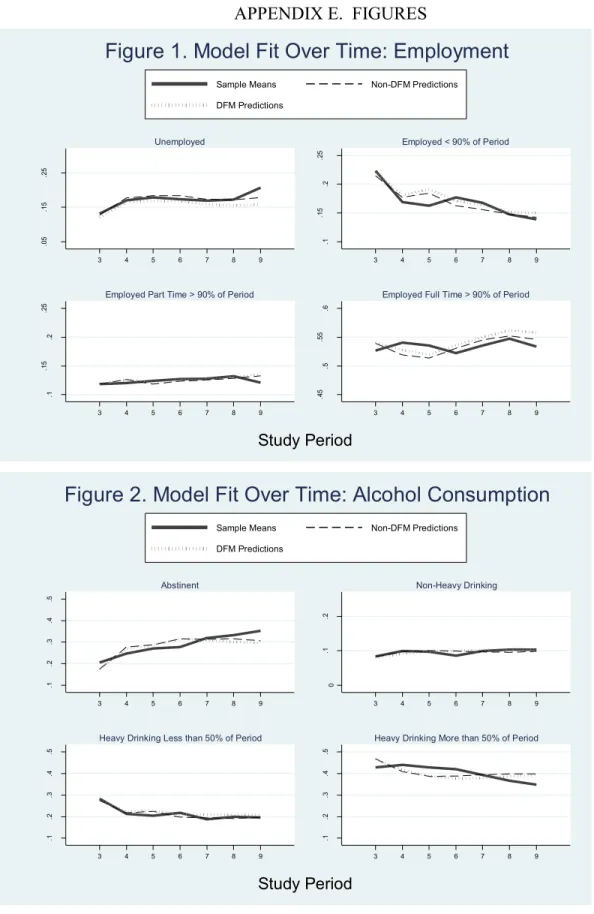
1. Model Fit Over Time: Employment ...136
2. Model Fit Over Time: Alcohol Consumption ...136
3. Model Fit Over Time: Alcohol Treatment Consumption ...137
4. Alcohol Outcomes Over Time by Alcohol Use During COMBINE Treatment ...137
5. Employment Outcomes Over Time by Alcohol Use During COMBINE Treatment ...138
6. Alcohol Outcomes Over Time by COMBINE Treatment ...138
7. Alcohol Outcomes Over Time by Lagged Employment ...139
8. Employment Outcomes Over Time by Lagged Employment...139
xii
LIST OF ABBREVIATIONS AA Alcoholics Anonymous
ACCRA American Chamber of Commerce Research Association AUD Alcohol Use Disorders
C2ER Council for Community and Economic Research CBI Cognitive behavioral intervention
COMBINE Combined Pharmacotherapies and Behavioral Interventions for Alcohol Dependence DFRE Discrete factor random effects
DSM-IV Diagnostic and Statistical Manual of Mental Disorders, 4th Edition
FDA Food and Drug Administration IC Initial condition
MH Mental health
MSA Metropolitan Statistical Area
NCAIS North American Industry Classification System NHIS National Health Interview Survey
NIAAA National Institue of Alcoholism and Alcohol Abuse and Drug Abuse NPD Non-Problem Drinking
NSDUH National Survey on Drug Use and Health
xiii OPC Outpatient Counseling
PDL Problem Drinking <50% of Period PDH Problem Drinking >50% of Period Q-F Quantity and frequency
RA Rational addiction
RCT Randomized Controlled Trial RxT Pharmacotherapy
SAMHSA Substance Abuse and Mental Health Services Administration
SH Self-help
CHAPTER I. INTRODUCTION
By the 21st century, 8.46% of adults in the United States met clinical criteria for alcohol abuse (4.65% or 9.7 million adults) or alcohol dependence (3.81% or 7.9 million adults) (Grant et al., 2004). Alcohol Use Disorders (AUDs), including abuse and
dependence, impose significant costs on society, estimated at $230 billion in 2009
(Rehm, 2009; Harwood, 2000; Mokdad, 2004). The majority of the cost burden (60%) is due to alcohol’s adverse impact on the labor market in the form of lost wages for those not employed and decreased productivity for those employed. It has been shown that alcohol abuse (MacDonald and Shields, 2004, Feng et al., 2001; Mullahy and Sindelar, 1996) and dependence (Johannson et al., 2007) are associated with unemployment and labor market detachment. AUDs are associated with lost productivity (Cook and Moore, 1999; Mullahy and Sindelar, 1998) and lower earnings (Keng and Huffman, 2002; Jones and Richmond, 2006; Zarkin et al., 1998). Understanding the causal relationships between alcohol and labor market performance is valuable for constructing alcohol use, prevention, and treatment policies.
2
and labor market success.1 The value of this literature is that it has identified AUDs as a measurable problem and has broadly described its costs to individuals and society.
The literature, however, has several limitations. Most studies are based on a snapshot of current substance use and labor market outcomes, ignoring how changes in both behaviors evolve over time and how the compositions of the AUD and non-AUD samples change (MacDonald, 2004).2 Economic decision making has a direct bearing on how the costs of substance abuse are determined, and understanding that behavior directly informs policy (Caulkins and Nicosia, 2010). Finally, it does not incorporate the role of AUD treatment in changing the composition of the AUD and non-AUD
populations that are compared in static cross-sections.
The second type of literature broadly focuses on the efficacy and effectiveness of prevention and treatment of AUDs (Room et al., 2007). These studies are generally based on clinical trials of interventions and specialty treatment and evaluations of programs or policies that directly provide treatment, reduce barriers to treatment, or create
disincentives for alcohol consumption. Labor market outcomes are usually analyzed as secondary outcomes in these studies. These studies are limited in their understanding of how improvements in AUDs lead to labor market outcomes and how those labor market outcomes recursively influence AUDs (e.g., psychosocial benefits of employment as a protective factor or work stress). Often, they are simply limited by the period of time over
1 These studies do not always compare two discrete populations, those with and those without AUDs, but
estimate local average treatment effects and implicitly compare populations with marginally different AUDs.
2 Johannson (2006) shows, for example, that currently abstinent, previously dependent drinkers often have poor
3
which they follow participants and do not allow sufficient time for improvements in labor market outcomes. Moreover, studies of specialty treatment often ignore the extent to which participants seek additional or future treatment beyond the original study. Yet, additional or repeated treatment is considered appropriate and is often based on attained employment which provides insurance or financial accessibility (CSAT, 2004).
In the study, I develop a model of employment, drinking, and treatment-seeking that is based on an economic model of individual behavior. The model is estimated using longitudinal data on individuals from a National Institute of Alcoholism and Alcohol Abuse and Drug Abuse (NIAAA) randomized control trial of two pharmacotherapies and a cognitive behavioral intervention (CBI) for dependence called Combined
Pharmacotherapies and Behavioral Interventions for Alcohol Dependence (COMBINE). The first aim of this study is to estimate the causal effects of AUD outcomes on
employment over a three-year period following the COMBINE trial. The second aim is to estimate the effects of employment outcomes on subsequent drinking. The third aim is to evaluate the role of ongoing therapy for AUDs. To this end, I develop a dynamic model that attempts to control for time varying and permanent heterogeneity and uses an identification strategy to reduce any bias from the endogenous relationships of these outcomes. Within this framework, I also evaluate several policy experiments related to the price of consumption goods and treatment as well as policies around treatment dosage.
4
CHAPTER II. BACKGROUND AND LITERATURE
Alcohol Abuse and Alcohol Dependence
Understanding what is meant by different AUDs is necessary for interpreting the literature on alcohol use and related outcomes. Moreover, the specific measures of AUDs can have different theoretical relationships with outcomes being studied. The Diagnostic and Statistical Manual of Mental Disorders, currently in its fourth edition (DSM-IV), provides clinical criteria for diagnosing alcohol abuse and alcohol dependence. Although various levels and patterns of alcohol consumption can be detected through biological screening (e.g., urine tests detect increased liver enzymes), DSM-IV clinical determinations are based on self-reported information. Indications of alcohol abuse are based on perceptions of drinking’s secondary effects: does the individual feel that alcohol caused problems at home, work, or school; led to dangerous behaviors; or led to criminal justice interactions. In addition, if the individual reports the inability to reduce consumption despite the perception of alcohol’s consequences he qualifies as abusing.
The DSM-IV defines dependence with a focus on consumption patterns, drinking’s primary consequences, and the individual’s relationship with alcohol. A positive diagnosis of dependence is typically made when a clinician identifies three or more of the following: (1) Spent a great deal of time over a period of a month getting, using, or getting over the
effects of alcohol;
6
(3) Needed to use alcohol more than before to get desired effects or noticed that same amount of alcohol use had less effect than before;
(4) Inability to cut down or stop using alcohol every time tried or wanted to; (5) Continued to use alcohol even though it was causing problems with emotions,
nerves, mental health, or physical problems;
(6) Alcohol use reduced or eliminated involvement or participation in important activities; and has experienced two or more withdrawal symptoms during the same time period:
(7) Reported experiencing two or more alcohol withdrawal symptoms at the same time that lasted longer than a day after alcohol use was cut back or stopped. Symptoms include (i) sweating or feeling that heart was beating fast, (ii) having hands tremble, (iii) having trouble sleeping, (iv) vomiting or feeling nausea[ted], (v) seeing, hearing, or feeling things that were not really there, (vi) feeling like could not sit still, (vii) feeling anxious, and (viii) having seizures or fits.3
It is important to recognize that abuse and dependence are psychological constructs that categorize a degree of severity in drinking behaviors, drinking consequences, and an individual’s relationship to drinking. AUDs represent a measurement problem described originally in psychological research in which a latent construct (e.g., dependence) is not observed but can be defined by how it manifests itself in behavior, consequences, and perceptions. AUDs are uniquely challenging to define because they are dynamic. Over time, individuals may cycle in and out of different levels of severity, even returning to abstinence. These observed cycles are not a reflection of the reliability of clinical testing
7
but are in evidence when measured by self-reported consumption patterns, clinical interviews, and biological screening (McLellan, 2007).
A special challenge for researchers is determining which measurement is useful for analysis. Consumption levels are correlated with the severity of a disorder as defined by the other criteria but their inconsistency has implications for some research questions. Clinical interviews have the advantage of evaluating an individual’s ongoing struggle with an AUD (e.g., strong cravings to drink or a fixation on alcohol) that may not be manifested through current consumption alone. For example, a currently abstinent individual may still have a latent disorder that is reducing his functioning or altering his preferences. In the first case, cross-sectional analyses of drinking and labor market outcomes would only represent the direct impact of drinking and the impact of disorders only for current drinkers. Altered preferences largely explain such phenomena as continued treatment seeking by abstainers as well as their avoidance of certain social environments (e.g., weddings with open bars). Longitudinal observation of consumption resolves these challenges to some extent while also providing more specificity (i.e., timing, lagged consumption patterns) than discrete clinical diagnoses.
In addition to the DSM-IV diagnosis criteria and in response to the public health burden of moderately risky drinking, researchers have also developed screening
instruments to detect both finer levels of less risky drinking while remaining sensitive enough to detect severe problems with minimal respondent information.4 Most screeners ask about an individual’s average alcohol consumption in standardized drinking units, usually the quantity of drinking in an episode and the frequency of episodes during a set
4 For example, the Alcohol Use Disorders Identification Test (AUDIT) is designed to detect a continuum of
8
time period. They also ask about perceptions of drinking and related consequences. Although consumption measures seem crude, they tend to be strong indicators of non-consumption criteria. In fact, there is an emphasis among public health and clinical researchers to move to a core quantity and frequency (Q-F) measure to more quickly screen individuals (Saitz, 2005; Gastfriend et al., 2007; McLellan, 2007). These
instruments and Q-F measures are prevalent in many large observational studies and have been used to estimate the relationship of drinking with secondary outcomes. Again, the use of reported consumption is often more appropriate in models of alcohol’s causal impact, since the alternative constructed measures described above often include the measures of the dependent variables being analyzed (e.g., absences from work).
Following from these different measures of drinking disorders, terms like ‘risky’, ‘problem’, ‘harmful’ or ‘hazardous’ drinking are used in different studies and are
sometimes used interchangeably with ‘abuse’. In the remainder of this literature review, I use the exact measures that the authors used and clarify their meanings when necessary. In the theoretical model described in Chapter 3, AUD is a continuous variable
representing the severity of an individual’s drinking disorder. In Chapter 4, I describe the primary measure of drinking that I use in my empirical model.
Employment and Drinking
AUDs are associated with labor market outcomes along multiple causal pathways. Both acute alcohol abuse, such as binge drinking, and longer term dependence can reduce an individual’s work productivity through reductions in human capital, health, and
9
Even if real productivity decreases are not realized, such drinking behaviors can serve as a negative signal to current and prospective employers. These adverse effects accumulate over time with increasing productivity loss and a growing portfolio of negative signals that can include sporadic labor market attachment and a reputation of low productivity.
AUDs may be associated with labor market outcomes through the individual’s preferences. An abusive or dependent drinker may value leisure differently because of worse health or a complementarity of drinking and leisure (Mello and Mendelson, 1972). He may discount time differently or have a different attitude toward risk, relative to the general labor market population either due to pre-existing characteristics or due to neurological changes brought on by drinking [Dom et al., 2005; Moselly et al., 2001; Tavares et al., 2004]. Therefore, he may leave the labor market more often and for longer periods of time. He may choose to work part time which may have later consequences for his earnings profile and employment probabilities. Alternatively, the deleterious effects of AUDs on health may provide more incentive for an individual to remain with an employer who provides health insurance.
10
encourages drinking. Finally, employment may provide protective factors that reduce the prevalence of AUDs. These include social norms that encourage safe drinking, wellness programs, and easier access to treatment through employer provided insurance and Employee Assistance Programs.
In this study, I focus on employment as the primary labor market outcome for several reasons. Employment is the broadest measure of labor market value and subsumes labor supply. For individuals currently in the labor market, real wages do not change much over a several-year time horizon. On the other hand, choosing to seek employment and finding employment are both outcomes with substantial variation over the study period.
Most of the estimated effects of AUDs on employment found in the economics literature rely on large, cross-sectional datasets. Specifically, these studies explain the different rates of employment between individuals with and without AUDs among an observed population.5 The fundamental econometric challenge in these studies is estimating the causal effects of AUDs in the face of a simultaneity problem or when unobserved heterogeneity is likely to explain both the AUD and labor market success. The standard approach in these studies is to use instrumental variables (IV) that predict an individual’s AUD but are theoretically and empirically uncorrelated with labor market outcomes other than through the AUD. With data from the National Health Interview Survey (NHIS), Mullahy and Sindelar (1996) used parental AUDs and beer and cigarette taxes as instruments of dependence, abuse and harmful drinking. MacDonald and Shields (2004) used non-acute illnesses that might limit drinking (e.g., asthma and diabetes) as
5
11
instruments of dependence in the 2000 National Health Survey of England. Johansson et al. (2007), using Finland’s Health 2000 survey, utilized parental characteristics, asthma and diabetes, religiosity, a person smoking behavior at the age of 18, and medical
biomarkers as instruments of dependence. All of these studies found significant and large effects of abuse and dependence on employment. Several found a positive relationship between moderate levels of drinking and employment.
One study (Feng et al., 2001) used a repeated cross-sectional dataset to estimate the effect of problem drinking on employment. Problem drinking was defined by
combinations of lifetime DSM-IV criteria and drinking behaviors during the previous 12 months. Employment was defined as any employment during the same 12 months. With data from the Epidemiological Catchment Areas of six southern US states, they estimated bivariate probit models of the contemporary effect of problem drinking on employment. When using county alcohol sales policies as instruments this study found no negative consequences of problem drinking on employment and argued that the effects of problem drinking on employment may occur over a long period of time.
12
employment consequences of an AUD last, we cannot know to what degree we may be underestimating the effect of having an AUD. Moreover, without understanding the causal mechanisms, we do not know whether we should expect prevention or treatment policies to have any short or long term labor market benefits. The only panel study of the AUD-employment relationship highlights this problem by offering the explanation that there may be a delay in employment consequences of problem drinking.
Treatment for Alcohol Use Disorders
In 2010, the number of persons aged 12 or older needing treatment for an alcohol use problem was 18.5 million (7.3 percent of the population aged 12 or older). Of these, 1.6 million (0.6 percent of the total population and 8.5 percent of the people who needed treatment for an alcohol use problem) received alcohol use treatment at a specialty
facility. Thus, there were 17.0 million people who needed but did not receive treatment at a specialty facility for an alcohol use problem. Among the 17.0 million people aged 12 or older who needed but did not receive treatment for an alcohol use problem in 2010, there were 698,000 (4.1 percent) who felt they needed treatment for their alcohol use problem. Of these, 485,000 did not make an effort to get treatment, and 213,000 made an effort but were unable to get treatment in 2010 due to lack of health coverage/cost of treatment, and/or lack of transportation (NSDUH, 2010).
13
criminal involvement. More detail on the sample is provided in Chapter 4. The three treatment options that I focus on are self-help (SH), outpatient counseling (OPC) and pharmacotherapy (RxT) which represent the majority of treatment sought by study individuals in the US. They also represent the most common treatment consumed by substance use treatment seekers in the US with 54% attending a SH group and 42% receiving OPC during a 12 month period (NSDUH, 2008). More importantly, these three modalities are of interest because of the way in which they fit lifestyles. The time and monetary costs of these are low relative to inpatient and residential treatment.
Individuals can continue working, living in their own residence and otherwise
functioning ‘normally’ while consuming these. Increasingly, an individual can seek OPC or RxT starting with their primary care physician and can avoid the stigma associated with traditional treatment. Along the continuum of AUD severity, there is a role for any of these. Even for the most severe AUDs, ongoing use of SH, outpatient and RxT should be considered following other more intensive therapies. Finally, their flexibility and relatively low costs make them ideal subjects for public health policy.
This chapter also provides the clinical basis for how treatment fits in the theoretical model presented in Chapter 2, including the justification of modeling
treatment as a stock. I describe the dynamics of treatment and the recovery. The chapter ends with the economic theory of treatment demand.
Defining Recovery
14
the goal of individuals seeking treatment (McLellan, 2004). Overall, specialty treatment for alcohol is effective with some studies finding more than half of recipients remaining abstinent by the end of the observation period (CSAT, 2004; Room et al., 2005; Project Match Research Group, 1997). Although many studies use length of time to relapse as an outcome, relapsing to problem drinking does not mean that the recovery process has ended and returning to treatment is not a bad outcome. Initial abstinence is a good predictor of long term healthy behaviors (Maisto et al., 2006; McKay and Weiss, 2001) including the maintenance of safe or controlled levels of drinking after treatment (McLellan, 2004; Gastfriend et al., 2007).
For an individual with a more severe AUD, ‘recovery’ is often defined by more than an episode of abstinence or controlled drinking. As noted earlier, consumption is useful for measuring outcomes over the limited periods of observation that studies face. However, clinicians, patients and researchers recognize that recovery is not simply an end state in which a ‘disease’ has been ‘cured’.6 Rather, language such as ‘in recovery’ is more commonly used to refer to ongoing success with an acknowledgement of the potential for relapse. Moreover, successful recovery is better conceived of as a steady state in which not only consumption is controlled but the latent factors that motivate problematic consumption are also alleviated or managed. These factors include antecedent individual characteristics such as genetics and socioeconomic environment that led to the initial AUD. Manifestations of these are risk- or sensation-seeking personalities, depression, anxiety and other psychiatric disorders, social acceptability of excessive drinking, social norms regarding leisure activities, and limited opportunities for healthy or fulfilling activities are all risk factors for AUDs that may remain in place even
15
after initial treatment has led to abstinence or controlled consumption. Dynamic factors brought on by past consumption also challenge the recovery process. These include changes in brain structure that alter decision-making faculties and alter preferences for alcohol and other goods and activities; development of mental illness; habits; and socioeconomic circumstances such as reduced human capital or a primary social group that is centered on alcohol. The broader goal of treatment is therefore to facilitate a steady state of recovery by managing these factors in addition to managing consumption.
Traditional Specialty Treatment and Self-Help
Conventional forms of specialty treatment vary by the severity of the AUD and most types of treatment may be considered part of a continuum of care that ideally helps an individual improve from his current AUD to steady state recovery. The intensity of
treatment in the continuum is intended to match the severity of the AUD and decreases as an individual improves. The intensity is loosely correlated with consumption level, due in part to the biological nature of severe physical addiction. The most intensive care associated with AUDs a period of detoxification in which a patient is sequestered, monitored and medicated for safety and management of withdrawal symptoms. Inpatient is traditionally 28 days and nights of treatment in a facility that offers a range of services, including RxT and counseling.
16
development of self-efficacy through ‘practicing’ sobriety. They also encourage proactive restructuring of an individual’s lifestyle. These include changes to work and social environments as well as developing alternative leisure activities. An individual is also encouraged to simultaneously treat mental or physical illness. Each approach seeks to change motivations by changing perceived social norms and reiterating the consequences of consumption, promoting positive social reinforcement and accountability (either from the family, a mentor or the clinician) and highlighting the positive value gained from alternative activities. They teach mechanisms for coping with stress and temptation, which include pre-commitment strategies (e.g., requesting hotel rooms without mini-bars) and contemporaneous coping strategies (e.g., cognitive tools for overcoming periods of temptation) (Moos 2007; Project Match Research Group, 1997).
Self-help groups, e.g., Alcoholics Anonymous (AA), are similar to OPC in several ways. Although they mostly employ some version of 12-step facilitation, the two modalities share many active ingredients as described in the preceding paragraph. Frequency of
sessions can be much higher for SH groups than for OPC, especially since they are virtually free. The culture of the therapy is the largest difference. SH groups are almost entirely composed of other individuals who are in recovery themselves (Peers) and usually have no formal clinical training. Despite some professional antagonism between SH organizations and clinical counselors, SH is often encouraged as a complement to formal specialty treatment or an alternative when an individual does not have the desire or means.
17
Pharmacotherapies are often prescribed in conjunction with inpatient treatment and OPC. Moreover, some of these medications are increasingly prescribed by primary care physicians for individuals with varying AUD severity and who may not otherwise be engaged in specialty substance abuse treatment. The medications commonly associated with AUDs typically fall into three categories: medications that alleviate withdrawal symptoms, medications that enhance overall mental health (MH), and medications that support recovery by directly influencing an individual’s preferences for drinking (Williams, 2005). The last group is the focus of this study. Medications for withdrawal are prescribed for a short period of time to reduce the mental and physical effects of sharp reductions in alcohol consumption. The broadest class used is benzodiazepines which have anxiolytic and anticonvulsant properties. It should be noted that the availability of medically facilitated detoxification and medications to make withdrawal less unpleasant can have a perverse effect on long run recovery as it reduces the disincentives to relapse and escalation of consumption. Moderate and severe MH problems are commonly co-occurring with AUDs, with anxiety and moderate depression having the highest
prevalence at all degrees of AUD severity. Regardless of the causal relationship between AUDs and MH, treating MH is expected to facilitate recovery indirectly by improving the individual’s overall wellbeing, his ability to cope, and by reducing the ‘pain’ of poor MH that leads to self-medication with alcohol. In other words, the intent is for these
18
(Berglund et al., 2006; Grant et al., 2004; Sher, 2004; Watkins et al., 2006). Their use is complicated by contraindications with drinking and, in the case of benzodiazepines, the specific concern of exposing individuals to new addictive substance. There is ample evidence that individuals seek these medications regardless of any intent to alter their alcohol consumption and that primary care physicians prescribe them without knowledge of an existing AUD. Because of this confounding and substantial use in the COMBINE sample, use of antidepressants, principally SSRIs, is included as a treatment consumption choice separate from other alcohol-specific treatments.
Medications in the third category are intended to support recovery directly and are usually prescribed specifically for the AUD. They theoretically aid recovery by reducing cravings, preventing compulsive relapse, or causing nausea or discomfort from drinking. There are currently three US Food and Drug Administration (FDA)-approved medications for relapse prevention during recovery from alcohol dependence: Disulfiram (Antabuse), Naltrexone and Acamprosate. As post-withdrawal pharmacotherapies, they function in a
gamma-19
aminobutyric acid (GABA) system. Acamprosate does not alter the effects of consumed alcohol. Acamprosate is the newest of the three drugs and was approved by the FDA in 2005. Several additional medications with similar pharmacology are either currently being studied for efficacy in managing drinking or are known to be prescribed off-label. These include quetiapine, topiramate, gabapentin, levetiracetam, baclofen, tiapride, bromocriptine and aripiprazole. Because certain benzodiazepines are γ-aminobutyric acid (GABA)ergic there is ongoing interest in their use as a longer run RxT for alcohol dependence despite the challenges described above (Bankole, 2005). Finally, serotonergic medications continue to be studied explicitly for treating alcoholism. There is some evidence that SSRIs are effective for controlling alcohol consumption especially for late-onset dependents. However, there is conflicting evidence as to whether the reduced preference for alcohol observed is due to a general effect on consumption and satiety with respect to food and liquids or a selective effect on alcohol. Moreover, there is little evidence that SSRIs are more beneficial for individuals with co-morbid depression than placebo in reducing alcohol abuse. Ondansetron is a serotonin antagonist (rather than an SSRI) with growing evidence of efficacy for drinking outcomes and also reported reductions in the cravings for alcohol and enjoyment of drinking.
Naltrexone, Acamprosate and this latter group of medications can have a proximal effect on alcohol consumption-both the decision to engage in drinking and the intensity of drinking. There is no set recommendation for how long Naltrexone and Acamprosate should be prescribed. The COMBINE trial dispensed medications for 4 months, while some
clinicians have recommended 6-12 months (Fatemi and Clayton, 2008). Disulfiram is usually prescribed for shorter periods. For all of them, there is an understanding that
20
longer run influence on recovery is expected to operate indirectly. Short run reductions in consumption allow the brain and physiological adaptations of addiction to heal and
normalize. While on the medications, lifestyle changes and habit formation may occur more easily and individuals may develop coping strategies. Their influence can function in a way dissimilar to counseling therapy alone. While on the medications, an individual may be able to manage his drinking while not altering his lifestyle, an often infeasible challenge. He can thus be reconditioned to not drink in response to the cues and routines of daily life.
Economic Models of Treatment for Alcohol Use Disorders
Any attempt to model an individual’s drinking, and treatment decisions must recognize that they are not made in ignorance of future consequences. An individual knows that abusive drinking can lead to near term and long term productivity loss, labor market challenges, poorer health and, most importantly, to severe dependence, a
proclivity for continuing abuse or withdrawal effects. The latter consequence, that individuals know that drinking today influences the value of drinking later, is a key component of Becker and Murphy (1988)’s rational addiction (RA) framework for modeling substance use. This framework is a useful starting place for analyzing drinking choices jointly with other economic choices. Drinking decisions today may be
influenced by expectations about productivity losses, employment probabilities and health. Moreover, individuals may recognize that consuming specialty treatment for AUDs can be an effective tool for moderating their drinking and its ultimate
consequences.
21
original theory did not explicitly make the case for treatment seeking. Orphanides and Zervos (1996) provided a rationale for a posterior demand for treatment, after an
individual discovered if they were an addictive personality type. Analogous justifications come from present-biased preferences (Gruber and Koszegi, 2001) and “projection bias” (Lowenstein, 1999) in which individuals assume that their current and future preferences will be similar. Several observed phenomena were still lacking theoretical justification, including relapse to AUDs, ongoing treatment seeking even after achieving abstinence, the tendency for some individuals’ convergence to moderate drinking patterns rather than abstinence. Bernheim and Rangel (2004), building on Laibson (2001), incorporate the neuroscience on substance use behavior into a traditional RA framework. A key
component is that individuals can find themselves seemingly randomly in a ‘hot’ mental state in which their instantaneous marginal utility of a substance leads to behavioral ‘mistakes’ and a reduction in total lifetime utility. The ‘hot’ states are brought on by environmental cues that trigger brain mechanisms that are manifested as a compulsive desire to consume the substance. In the Bernheim and Rangel model, individuals in recovery manage this challenge in part by choosing safe environments in which the flow of cues is reduced. The most extreme example of this behavior is checking into a
residential treatment facility. A second role of treatment that their model recognizes is learning to deal with cues, a common objective of most counseling therapy. Although they do not discuss RxT, it can be justified in a similar way as counseling.
In the traditional RA framework, treatment has primarily been presented as an investment in future outcomes at the expense of current utility from leisure and
22
e.g., through social interactions or self-empowerment. As described above, treatment may alter the immediate marginal utility of drinking or time preferences (Yoon et al., 2007). It may similarly alter the experience of and thus preferences for leisure and other consumption. For example, Naltrexone has been reported to reduce the enjoyment of shopping. Gul and Pesendorfer (2007) provide an alternative model of addiction that subsumes these latter effects of treatment on utility. In their framework, utility is a function of both actual consumption and the individual’s remaining choice set. Although this framework somewhat ignores how treatment alters the utility of all other
consumption and leisure, it clearly justifies including treatment as an input to current utility.
In summary, recent theoretical literature has developed models of the demand for treatment that fit better with observed data. They are consistent with several stylized facts and with findings in the clinical literature: individuals vary in their substance use patterns. The behaviors of some individuals are consistent over long periods of time, while others are dynamic, cycling through dependence, moderation, and abstinence. Individuals seek treatment all along the continuum between dependence and abstinence. Almost all of the models of addiction are underidentified by available data. Nonetheless, the economic models are consistent in their implication that under certain assumptions individuals may seek treatment.7
The policy relevance of studying treatment is threefold. First, there are externalities from AUDs, including decreased employment and lost productivity, accidents, public health care costs, and crime. Second, the existing treatment system is largely a public system. Given that some individuals are willing to seek treatment, it is
23
worthwhile to study the relative effectiveness of different portfolios of treatment to inform policies that promote treatment. Interest in RxT is particularly high because it is a passive and convenient form of treatment that can be prescribed by primary care
physicians which reduces the overall stigma of receiving treatment (Bankole, 2005).8 Finally, as synopsized by Bernheim and Rangel (2004) individuals may suffer from unanticipated compulsion to consume sub-optimally (internalities). Studying the effectiveness of alternative treatments is worthwhile for improving their welfare.
CHAPTER III. THEORETICAL MOTIVATION
In this section I present a dynamic, theoretical model of the behavior of individuals who have had an AUD and who have previously sought formal specialty treatment for the AUD. Chapter 4 will provide greater detail concerning the study sample, but two characteristics of the data provide useful context for the theoretical model. First, each time period in the data is roughly four calendar months which is the time between data collection interviews. Second, at the time of the interview, questions about employment, outpatient counseling and self-help sessions are reported as totals for the entire period, whereas drinking and pharmacotherapy to manage drinking and
depression are reported for each day within the period. The model focuses on their employment, drinking, ongoing AUD treatment decisions and the use of antidepressants.
In each period t, an individual maximizes his remaining lifetime expected utility by choosing per-period hours of general leisure, lt, levels of alcohol consumption, at, types of therapy to manage drinking and the AUD (including no therapy), mt, whether or not to consume antidepressants, st, and amount of consumption, ct. He begins each
period with a set of state variables accounting for his previous decisions and experiences: work history prior to the current period, Qt; drinking history, At; past treatment choices,
Mt; past antidepressant use, St; and, Dt, the current level of severity of his AUD. A
25
influences the marginal utilities of the choice variables in the immediate period. The individual receives negative utility from experiencing any level of AUD (Dt), which
can be conceptualized as the subjective disutility of having a high addictive stock, negative psychic consequences of alcohol abuse, or guilt and frustration over drinking behaviors. An individual’s work, alcohol use, treatment, and antidepressant stocks at the beginning of period t are functions of the respective stocks at the beginning of the
previous period and his employment, alcohol use, AUD treatment, and antidepressant use in period t-1
His AUD, Dt, is a function of all his current-state variables, particularly drinking history (At), and the previous level of AUD, Dt-1,
) , , ,
( 1 ,
D t t t t
t D D A M S
D (1)
Dt may also influence the marginal utilities of the choice variables.
The marginal utility of drinking (at) is conditional on the current treatment
consumption (mt) which reduces the marginal utility of alcohol; drinking history (At), a standard feature in rational addiction models; previous treatment that forms a stock of capacity to moderate drinking (Mt); past antidepressant use (St); and the current severity
of the AUD (Dt). Thus past drinking (At) affects the current drinking choice through the
typical addiction/habit formation mechanism as well as indirectly through the AUD for which an individual may drink to cope or relieve the psychic distress.
The vectorZt includes observable local environmental characteristics such as wages by sector, prices, and local treatment capacity. Xtis a vector of observable
26
unobserved time varying factor and i,tis the idiosyncratic error. For notational ease in the utility function, i subscripts for individual are left out of the model. Also, let Kt be the vector of all the state endogenous variables: (Qt,At,Mt,St,Dt).
At each time period t, the individual selects lt, at, mt , st, and ct to maximize expected discounted utility realizing that in the future the individual will make the optimal choice given the realized values of the random variables, with T being the last period of the individual’s life.
1[ ( , , , , ; , , , , , )]
1 t t t t t t t t t t
t T t
t U a l m s c K X Z
(2)
subject to a maximum number of hours (3), four laws of motion (4-7), a production function for the AUD severity (8), a budget constraint that does not include borrowing (8), and a wage offer (10):
Ω- lt = ht (3)
) , ,
( 1 1 Q
t t
t Q l Q
Q (4)
) , ,
( 1 1 A
t t
t A a A
A (5)
) , ,
( 1 1 M
t t
t M m M
M (6)
) , ,
( 1 1 S
t t
t S s S
S (7)
) , , ,
( 1 , D
t t t t
t D D A M S
D
(8)27
) , , ( t t t
t w K X Z
w (10)
The variable β is a constant discount factor. Ω is the maximum hours available to the individual in each time period. The j in equations 4-8 are depreciation rates for their
respective state variables. pa,t, pm,t, and ps,t are the prices of alcohol, AUD treatment and
antidepressants, respectively. wt is the individual’s wage if working, and Ntis any
non-labor income. Ut is a concave function of current drinking, leisure, treatment,
antidepressant use and other consumption. For a large range of drinking levels, Ut is an
increasing function ofat, though it is possible that the marginal effect of alcohol
eventually becomes negative. Assuming that utility is an increasing, concave function of
t
a , the signs of the partial derivatives are
; 0 ) , , , , , , ; , , , , ( t t t t t t t t t t t t a Z X D K c s m l a
U
(11) 0 ) , , , , , , ; , , , , ( 2 2 t t t t t t t t t t t t a Z X D K c s m l a
U (12)
t t t t t t t t t t
t l m s c K D X Z
a, , , , , , , , ,, ,
All of the state variables are increasing functions of their respective past outcomes and they depreciate. Consistent with the standard rational addiction framework, current drinking (at)
influences the marginal utility of future drinking via an increment in the state variable At+1
used in the following period. AUD severity, Dt, is a function of past AUD severity, as well
28
By assumption, an individual’s marginal utility of alcohol consumption increases with the drinking history state variable (At):
0 ) , , , , , , ; , , , , ( 2 t t t t t t t t t t t t t a A Z X D K c s m l a
U
(13) t t t t t t t t t t
t l m s c K D X Z
a, , , , , , , , ,, ,
and decreases with past treatment (Mt):
0 ) , , , , , , ; , , , , ( 2 t t t t t t t t t t t t t a M Z X D K c s m l a
U
(14)
29
In the BM model, the motivation to reduce consumption is based primarily on the secondary consequences of chronically high levels of drinking such as health, productivity, crime, or changes in the price of alcohol. By emphasizing the per se disutility of having an AUD, the model diverges from BM conceptually but is not inconsistent in its general predictions. The labor market is the only consequence that I explicitly include in the model and is described below. As noted earlier, I am allowing current treatment to directly enter an individual’s utility function.
Clinical treatment, self-help, and pharmacotherapy as well as antidepressant use are special cases of the general effort spent to reduce drinking introduced by BM. In this model I ignore any non-formal treatment for three reasons. First, I do not observe any informal efforts. Second, all of the study subjects have engaged in formal treatment at some point in their lives. Almost all formal treatment has some component of therapy that teaches
individuals behaviors and habits to help them control their drinking and prevent relapse. All treatment requires a component of personal effort and encourages ongoing personal effort.9 Therefore, it becomes difficult to disentangle pure personal effort from any ongoing
treatment effect. Finally, because consumption of formal treatment, and especially
pharmacotherapy, can be more easily encouraged by policy-makers, estimates of its effect are of greater interest.
As described in Chapter 2, the Becker and Murphy and Orphanides and Zervos rational addiction frameworks do not by themselves predict several observed drinking and treatment seeking behaviors, especially over shorter periods of time. The models of Bernheim and Rangel and Gul and Pesendorfer offer better face validity; however, neither
9 Arguably, all personal effort after treatment is more productive because of the ‘technology’ acquired in
30
would significantly change the empirical model that I describe in Chapter 5 and that is supported by the data. Finally, this model does not explicitly include any learning or Bayesian updating by an individual concerning his addiction or treatment efficacy. Timing10
At the beginning of each period, t, the individual has complete information about his past and also about his current market environment:
past behaviors (Qt,At,Mt,St),
the current severity of the AUD (Dt),
current preferences which are influenced by past behaviors and a random preference shock,
current prices for alcohol, treatment, antidepressants, and consumption goods (Zt),
a current wage offer , wt, (including no offer) which is also a function of
the state variables.
10 I considered as alternative theoretical model in which individuals choose employment at the beginning of a
31
The values of the state variables, current preferences (after the preference shock is known), prices and the wage offer remain constant throughout the entire period. During the period, he simultaneously chooses employment status, how much to drink, how much AUD treatment to consume, antidepressant use, and other consumption. At the end of the period, state variables are updated based on those decisions.
The individual knows that the decisions made during the current period affect future preferences, particularly the future marginal utility of alcohol, through his state variables. He also knows that current decisions will affect future productivity, the probabilities of receiving future wage offers, the distribution of future wage offers, and the severity of the AUD in the future. The individual’s per-period decision making can be described by the following value function framework. Recall that Ktis the vector of
state variables which represent four laws of motion for employment, drinking, AUD treatment decisions and the use of antidepressants (Equations 4-7) and the AUD severity.
In the final period T of an individual’s life, consumption is chosen to maximize current utility with no consideration of future periods.
) , , , , , ; , , , , ( max )
, , (
, , ,
,l m s c T T T T T T T T T T
a T T
T U a l m s c K X Z
K V
T T T T T
(15)
In each period t<T, conditional on state variables (Kt) and the period t specific
32
T t K c s m l a K K t s K V E Z X K c s m l a U K V t t t t t t t t t t t t t t t t t t t t c s m l a t t t t t t t t t t ) ; , , , , ( . . ) , , ( ) , , , , , ; , , , , ( max ) , , ( 1 1 1 1 , , , , , 11
(16)
Since the per-period choices are made jointly, they are all functions of the same set of state variables, prices and community-level characteristics, individual
characteristics and heterogeneity. In each period, the employment decision (leisure demand), and demand for alcohol, AUD therapies, and antidepressants are
)
,
,
,
,
,
,
,
,
(
t t t t t tt
e
Q
A
M
S
D
Z
X
e
t t
(17))
,
,
,
,
,
,
,
,
(
t t t t t tt
a
Q
A
M
S
D
Z
X
a
t t
(18))
,
,
,
,
,
,
,
,
(
t t t t t tt
m
Q
A
M
S
D
Z
X
m
t t
(19))
,
,
,
,
,
,
,
,
(
t t t t t tt
s
Q
A
M
S
D
Z
X
s
t t
(20)Wages unconditional on employment are functions of the same variables except w
t
Z only includes market wages and excludes prices for consumption goods contained in
t
Z .
w t
X excludes non-labor income.
)
0
|
,
,
,
,
,
,
,
,
(
w t tt w t t t t
t
w
Q
A
M
S
D
Z
X
h
CHAPTER IV. DATA
COMBINE Study Sample
The COMBINE trial randomized 1,383 adult participants to nine different combinations of two pharmacotherapies (Acamprosate and Naltrexone) and a CBI. The trial also included Medication Management for all but one group that received no pills or placebos. Randomization took place within eleven different treatment sites in the United States between 2001 and 2003 (Medical University of South Carolina, Boston
Consortium, University of Washington, University of Texas, Brown University, University of Miami, University of New Mexico, Yale University, University of Pennsylvania, Harvard University, University of Wisconsin). Trial treatment lasted for sixteen weeks after which the individuals’ only interaction with trial staff was
incentivized follow-up data collection. Data collection continued at four-month intervals for three years after randomization for a subset of willing participants whose data were collected for an economic study of COMBINE. Nine of the original eleven sites chose to continue data collection for the economic study.
The main inclusion criterion for the study was a DSM-IV diagnosis of alcohol dependence. Participants were excluded if another substance was deemed to be the primary drug of dependence, had a severe psychiatric illness or had certain serious physical
34
and have two or more days of heavy drinking (defined as 4 drinks for females and 5 drinks for males) in the 90-day period prior to initiation of abstinence. Participants must have had a minimum of 4 consecutive days (96 hours) of abstinence. Participants can be abstinent for a maximum of 21 days prior to randomization.” Participants were also excluded if they intended to engage in any other treatment for alcohol-related problems during the 16 week study period, if they had used one of the study medications in the past 30 days or if they had had inpatient substance use treatment in the past 30 days.
In this study I focus on outcomes following the end of the 16 week trial for several reasons. Participation in a clinical trial artificially influences outcomes due to
inclusion/exclusion criteria, time commitments and frequent interactions with clinical staff. The study required up to four visits per month to the research site during the trial treatment. Second, I am using the trial’s randomization of individuals to treatment arms as an
identification strategy for the initial drinking and treatment conditions. Participation in the trial represents a reset of many individuals’ drinking profiles and also initiates them to different experiences with RxT.
Appendix Table A.1 describes the sample size and observations of the original COMBINE study. Of the 991 participants who completed 16 weeks of treatment in the nine sites that continued the study, 792 chose to participate in the three-year economic study and completed 6,138 interviews including an interview at randomization and at the end of 16 weeks of trial treatment. Attrition within this group was limited.11 Moreover, there were relatively few missing interviews because the data collection instruments were
11 The reasons for the low attrition rate include the frequency of follow-up interviews, incentives, the
rapport established between the study participants and the study staff during the main study period, and the amount of grant resources provided to the study sites to support data collection. Finally, the
35
designed to capture outcomes since the previous interview. The clinical staff conducting the interviews were trained in techniques to improve recollection (COMBINE Protocol). In accordance with the original study, if too much time passed between interviews, the clinical staff attempted to reconstruct the outcomes as of the time of the missed interview. Although this approach to data collection increases the likelihood of recall bias, it has the advantage of removing intermittent missing information. Fortunately, less than 6% of interviews occurred outside of 60 days of the intended interview date. Finally, there was virtually no non-response to any particular question in the primary data collection
instrument other than logical survey skips. The current analysis sample is 775
individuals with 4,994 post trial interviews after removing 17 individuals with a large number of inconsistent or missing observations or individuals with fewer than four of the eight possible follow-up interviews. Of these, 601 interviews were flagged as having been reconstructed. Appendix Table A.2 provides definitions for key model covariates.
36
interval time is useful because it not only supports a longitudinal and dynamic statistical model but it also supports a theory-driven statistical model that depends on simultaneous alcohol consumption and treatment decisions. In other words, it supports modeling the key behaviors that theory would predict. No other survey contains such detailed measures of treatment use, substance use, and employment outcomes over such fine periods of time.
Appendix Table A.3 describes the characteristics of the 775 individuals in the analysis sample. Marital status and education variables are both mutually exclusive categorical variables. Of note, this sample is fairly well educated with fewer than 7% not having achieved a high school degree or better, and over 40% having a college degree or higher. Marital status and education are only collected at the beginning of the trial, therefore I do not observe any changes over time.
37
whether it happened due to improvements in job search success or due to a stronger preference or capacity to supply labor. In the COMBINE sample, 96% (not reported in Appendix Table A.4) report either being employed or looking for employment in at least one time period. In any period a little over half of the sample is employed full-time for almost the whole period and another 12-13% are employed part-time for most of the period. The final three columns provide evidence of the variation in employment status over the three years of the study. Post-trial 75% of the sample was employed full-time for >90% of the period at least once. Thirty-three percent of the sample did not work at all during at least one period of reporting. Alternatively, only 40% of the sample did not change employment status. The largest group that remained the same was full-time for >90% of the period at 29%, followed by 8% who did not work the entire time. Although not reported in the table, over half of those claimed to have looked for work during at least one period. These facts are consistent with the inclusion/exclusion criteria which admitted a relatively high functioning group of individuals with AUDs.
Alcohol consumption was recorded in US standard drinking units (14 grams of alcohol) for each day during the look-back period. From these daily amounts I define a
38
period. The first is no drinking at all; the second is moderate or controlled drinking in which alcohol is consumed, but no problem weeks are reported. Among those who reported any problem weeks, I divide the group into those for whom less than half of the period was consumed of problem weeks and those who reported more than half of the period as problem weeks. Because of the inclusion criteria of the study, everyone in the sample was in a problem drinking category at Period 1. During the period of treatment, 21% of the sample remained abstinent with most individuals having problem weeks more than half of the period (36.9%). This latter category increased to 44.0% in Period 3, eight months after study treatment ended. Over time, the number of individuals reporting abstinence increases to 35.3% in Period 9, while the number of patients with any problem drinking decreases. Although some of this is due to sample attrition, some of it is due to recognized patterns of natural and treatment-supported recovery. The final column of Appendix Table A.5 demonstrates the drinking dynamics within individuals with 47.9% reporting at least one period of abstinence and 63.4% reporting at least one period of problem drinking greater than half the period.
39
reason is supported by the observed data. For example, 46 SH observations were
eliminated of which 37 were periods in which only one SH visit was reported. Similarly, for RxT, I included only periods in which more than 14 days of RxT were consumed. This amount ensured that the effects of any of the medications could have been in place based on known titration levels. Moreover, because there is evidence that individuals often choose to consume pharmacotherapies for discrete time periods either in response to AUD concerns or in anticipation of circumstances or events. This is most common with Disulfiram, but is also true for Naltrexone. Sixteen observations were not included as RxT, of which all had less than five days of consumption.
Since all of these modalities can be consumed simultaneously, I constructed a categorical variable that is reported in Appendix Table A.6. Because cell sizes were small for some combinations, the categorical variable was reduced to four categories: No treatment, SH only, OPC or OPC + SH, and RxT alone or in combination with OPC and/or SH. The non-mutually exclusive outcomes for each of the three treatment
40
Appendix Table A.8 presents transition probabilities for each of the dependent variables to further demonstrate variability over time. For employment, period full-time employment was the most persistent category with 84.5% remaining in this category across Periods 3-9. For alcohol, abstinence was the most persistent with 81.3% remaining abstinent if they were abstinent in the previous period. Very few individuals go from problem drinking (>50% of the period) to abstinence or moderate drinking in a single period. Similarly, only 3.8% of moderate drinking periods are followed by problem drinking (>50% of the period). Periods with no treatment are usually followed by periods with no treatment (89.6%).