Boxes
Karl Bringmann
1, Sergio Cabello
∗2, and Michael T. M. Emmerich
31 Max Planck Institute for Informatics, Saarland Informatics Campus, Saarbrücken, Germany
2 Department of Mathematics, IMFM, Ljubljana, Slovenia; and
Department of Mathematics, FMF, University of Ljubljana, Ljubljana, Slovenia
3 Leiden Institute of Advanced Computer Science (LIACS), Leiden University, Leiden, The Netherlands
Abstract
LetBbe a set ofnaxis-parallel boxes inRd such that each box has a corner at the origin and
the other corner in the positive quadrant ofRd, and letk be a positive integer. We study the
problem of selectingk boxes inB that maximize the volume of the union of the selected boxes. The research is motivated by applications in skyline queries for databases and in multicriteria optimization, where the problem is known as the hypervolume subset selection problem. It is known that the problem can be solved in polynomial time in the plane, while the best known running time in any dimensiond≥3 is Ω nk. We show that:
The problem is NP-hard already in 3 dimensions.
In 3 dimensions, we break the bound Ω nk, by providing annO( √
k) algorithm.
For any constant dimensiond, we give an efficient polynomial-time approximation scheme.
1998 ACM Subject Classification F.2.2 Nonnumerical Algorithms and Problems
Keywords and phrases geometric optimization, subset selection, hypervolume indicator, Klee’s measure problem, boxes, NP-hardness, PTAS
Digital Object Identifier 10.4230/LIPIcs.SoCG.2017.22
1
Introduction
Ananchored box is an orthogonal range of the form box(p) := [0, p1]×. . .×[0, pd]⊂Rd≥0,
spanned by the pointp∈Rd
>0. This paper is concerned with the problemVolume Selection:
Given a setP ofnpoints inRd>0, selectkpoints in P maximizing the volume of the union
of their anchored boxes. That is, we want to compute
VolSel(P, k) := max
S⊆P,|S|=kvol
[
p∈S
box(p),
as well as a setS∗⊆P of size krealizing this value. Here,voldenotes the usual volume.
Motivation
This geometric problem is of key importance in the context of multicriteria optimization and decision analysis, where it is known as the hypervolume subset selection problem (HSSP)
∗ Supported by the Slovenian Research Agency, program P1-0297 and project L7-5459.
© Karl Bringmann, Sergio Cabello, and Michael T. M. Emmerich; licensed under Creative Commons License CC-BY
[2, 3, 4, 24, 12, 13]. In this context, the points inP correspond to solutions of an optimization problem with d objectives, and the goal is to find a small subset of P that “represents” the set P well. The quality of a representative subsetS ⊆P is measured by the volume of the union of the anchored boxes spanned by points in S; this is also known as the
hypervolume indicator [34]. Note that with this quality indicator, finding the optimal size-k representation is equivalent to our problemVolSel(P, k). In applications, such bounded-size representations are required in archivers for non-dominated sets [23] and for multicriteria optimization algorithms and heuristics [3, 10, 7].1 Besides, the problem has recently received attention in the context of skyline operators in databases [17].
In 2 dimensions, the problem can be solved in polynomial time [2, 13, 24], which is used in applications such as analyzing benchmark functions [2] and efficient postprocessing of multiobjective algorithms [12]. A natural question is whether efficient algorithms also exist in dimensiond≥3, and thus whether these applications can be pushed beyond two objectives.
In this paper, we answer this question negatively, by proving thatVolume Selection
is NP-hard already in 3 dimensions. We then consider the question whether the previous Ω( nk) bound can be improved, which we answer affirmatively in 3 dimension. Finally, in any constant dimension, we improve the best-known (1−1/e)-approximation to an efficient polynomial-time approximation scheme (EPTAS). See Section 1.2 for details.
1.1
Further Related Work
Klee’s Measure Problem
To compute the volume of the union ofn(not necessarily anchored) axis-aligned boxes inRd
is known as Klee’s measure problem. The fastest known algorithm takes time2O(nd/2), which can be improved toO(nd/3polylog(n)) if all boxes are cubes [15]. By a simple reduction [8],
the same running time as on cubes can be obtained on anchored boxes, which can be improved toO(nlogn) ford≤3 [6]. These results are relevant to this paper because Klee’s measure problem on anchored boxes (spanned by the points in P) is a special case of Volume Selection(by callingVolSel(P,|P|)).
Chan [14] gave a reduction fromk-Clique to Klee’s measure problem in 2kdimensions. This proves NP-hardness of Klee’s measure problem whendis part of the input (and thus dcan be as large asn). Moreover, sincek-Clique has nof(k)·no(k) algorithm under the Exponential Time Hypothesis [16], Klee’s measure problem has nof(d)·no(d) algorithm
under the same assumption. The same hardness results also hold for Klee’s measure problem on anchored boxes, by a reduction in [8] (NP-hardness was first proven in [11]).
Finally, we mention that Klee’s measure problem has a very efficient randomized (1±ε )-approximation algorithm in timeO(nlog(1/δ)/ε2) with error probabilityδ[9].
Known Results for Volume Selection
As mentioned above, 2-dimensionalVolume Selectioncan be solved in polynomial time; the initialO(kn2) algorithm [2] was later improved toO((n−k)k+nlogn) [13, 24]. In higher
dimensions, by enumerating all size-k subsets and solving an instance of Klee’s measure problem on anchored boxes for each one, there is anO nk
kd/3polylog(k)
algorithm. For
1 We remark that in these applications the anchor point is often not the origin, however, by a simple
translation we can move our anchor point from (0, . . . ,0) to any other point inRd.
small n−k, this can be improved to O(nd/2logn+nn−k) [10]. Volume Selection is NP-hard whendis part of the input, since the same holds already for Klee’s measure problem on anchored boxes. However, this does not explain the exponential dependence onk for constantd.
Since the volume of the union of boxes is a submodular function (see, e.g., [31]), the greedy algorithm for submodular function maximization [27] yields a (1−1/e)-approximation of VolSel(P, k). This algorithm solves O(nk) instances of Klee’s measure problem on at mostkanchored boxes, and thus runs in timeO(nkd/3+1polylog(k)). Using [9], this running
time improves toO(nk2log(1/δ)/ε2), at the cost of decreasing the approximation ratio to 1−1/e−εand introducing an error probabilityδ. See [20] for related results in 3 dimensions.
A problem closely related toVolume SelectionisConvex Hull Subset Selection: Givenn points inRd, select kpoints that maximize the volume of their convex hull. For
this problem, NP-hardness was recently announced in the cased= 3 [28].
1.2
Our Results
In this paper we push forward the understanding of Volume Selection. We prove that
Volume Selection is NP-hard already for d= 3 (Section 3). Previously, NP-hardness was only known whendis part of the input and thus can be as large as n. Moreover, this establishes Volume Selection as another example for problems that can be solved in polynomial time in the plane but are NP-hard in three or more dimensions (see also [5, 26]).
In the remainder, we focus on the regime whered≥3 is a constant andkn. All known algorithms (explicitly or implicitly) enumerate all size-ksubsets of the input setP and thus take time Ω nk
=nΩ(k). In 3 dimensions, we break this time bound by providing annO(√k)
algorithm (Section 4). To this end, we project the 3-dimensionalVolume Selectionto a 2-dimensional problem and then use planar separator techniques.
Finally, in Section 5 we design an EPTAS for Volume Selection. More precisely, we give a (1−ε)-approximation algorithm running in timeO((n/εd)(logn+k+ 2O(ε−2log 1/ε)d
)), for any constant dimension d. Note that the “combinatorial explosion” is restricted to d andε; for any constant d, εthe algorithm runs in timeO(n(k+ logn)). This improves the previously best-known (1−1/e)-approximation, even in terms of running time.
2
Preliminaries
All boxes considered in the paper are axis-parallel and anchored at the origin. For points p= (p1, . . . , pd), q= (q1, . . . , qd)∈Rd, we say thatpdominates qifpi≥qi for all 1≤i≤d.
Forp= (p1, . . . , pd)∈Rd>0, we letbox(p) := [0, p1]×. . .×[0, pd]. Note thatbox(p) is the
set of all pointsq∈Rd
≥0that are dominated byp. Apoint set P is a set of points inRd>0.
We denote the unionS
p∈Pbox(p) byU(P). The usual Euclidean volume is denoted byvol.
With this notation, we set
µ(P) :=vol(U(P)) =vol [
p∈P
box(p)=vol [
p∈P
[0, p1]×. . .×[0, pd]
.
We studyVolume Selection: Given a point setP of size nand 0≤k≤n, compute
VolSel(P, k) := max
S⊆P,|S|=k
µ(S).
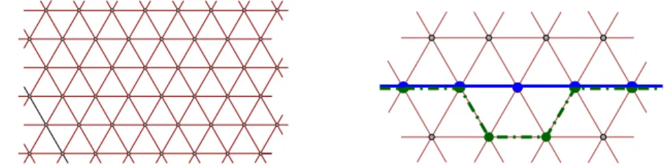
Figure 1Left: triangular grid Γ. Right: choosing the parity of paths.
3
Hardness in 3 dimensions
We consider the following decision variant of 3-dimensionalVolume Selection: Given a triple (P, k, V), whereP is a set of points inR3
>0,kis a positive integer andV is a positive
real value, is there a subsetQ⊆P ofk points such thatµ(Q)≥V?
We are going to show that the problem is NP-complete. First, we show that an interme-diate problem about selecting a large independent set in a given induced subgraph of the triangular grid is NP-hard. Then we argue that this problem can be embedded using boxes whose points lie in two parallel planes. One plane is used to define the triangular-grid-like structure and the other is used to encode the subset of vertices that describe the induced subgraph of the grid.
3.1
Triangular grid
Let Γ be the infinite graph with vertex set and edge set (see Figure 1):
V(Γ) =
(i+j·1/2, j·√3/2)|i, j∈N ,
E(Γ) = {ab|a, b∈V(Γ), the Euclidean distance betweenaandbis exactly 1}.
We use the problemIndependent Set on Induced Triangular Grid: Given a pair (A, `), whereAis a subset ofV(Γ) and`is a positive integer, is there a subsetB⊆Aof ` vertices such that no two vertices ofB are connected by an edge ofE(Γ)?
ILemma 3.1. Independent Set on Induced Triangular Gridis NP-complete.
Proof Sketch. Garey and Johnson [19] show that the problem Vertex Cover is NP-complete for planar graphs of degree at most 3, which implies thatIndependent Setis NP-complete for planar graphs of degree at most 3.
Given a planar graphGof degree at most 3, we construct an orthogonal drawing ofGon a square grid of polynomial size [29, 30] and transform it into a drawing ofGon Γ. Rescaling and rerouting, we get a graphH that is an induced subgraph of Γ, and a subdivision ofG where each edge ofGis path inH with an even number of interior vertices. See Figure 1, right, to see how to choose the parity of the path. Ifα(G) is the size of the largest independent set inG, and each edgeuvof Gis represented by a path with 2kuv internal vertices, then
α(H) =α(G) +P
uv∈E(G)kuv. Indeed, we can obtainH fromGby repeatedly replacing an
edge by a 3-edge path, and any such replacement increases the size of the largest independent
set by exactly 1. J
3.2
The point set
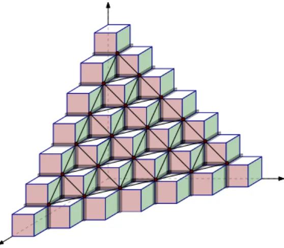
Letm≥3 be an arbitrary integer and consider the point setPmdefined byPm={(x, y, z)∈
N3 | x+y +z = m}, see Figure 2. Standard induction shows that the set Pm has
ε ε
ε ε
ε ε
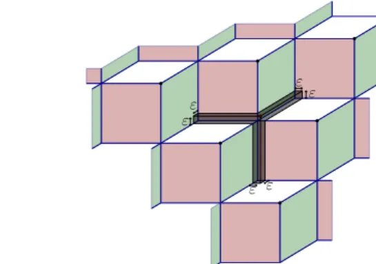
Figure 2Left: the point setPmand the boxesbox(p), withp∈Pm. Right: the pointq=p+ ∆ε
and the setdiff(q).
Consider the real numberε= 1/4m2, and define the vector ∆
ε= (ε, ε, ε). Note thatεis much
smaller than 1. For each pointp∈Pm−1, consider the pointp+∆ε, see Figure 2, right. Let us
define the setQm={p+ ∆ε|p∈Pm−1}. It is clear thatQmhas|Pm−1|= (m−2)(m−3)/2
points, form≥3. The points ofQmlie on the planex+y+z=m−1 + 3ε. For each point
qofQmdefine
diff(q) = U Pm∪ {q}\ U Pm =
[
p∈Pm∪{q}
box(p)
\
[
p∈Pm
box(p)
.
Note thatdiff(q) is the union of 3 boxes of sizeε×ε×1 and a cube of sizeε×ε×ε, see Figure 2, right. The sets and the parameterεare selected to have the following properties.
ILemma 3.2. The following holds.
If Q0 ⊆Qm and the setsdiff(q), for allq∈Q0, are pairwise disjoint, thenµ(Pm∪Q0) =
µ(Pm) +|Q0| ·(3ε2+ε3).
If Q0 ⊆ Qm and Q0 contains two points q0 and q1 such that diff(q0) and diff(q1) intersect, thenµ(Pm∪Q0)< µ(Pm) +|Q0| ·(3ε2+ε3).
If P0 is a subset ofPm such thatPm\P0 is non-empty, thenµ(P0∪Qm)< µ(Pm).
3.3
The reduction
We can define naturally a graph Tm on the set Qm by using the intersection of the sets
diff(·). The vertex set ofTmisQm, and two pointsq, q0∈Qm define an edgeqq0 ofTm if
and only ifdiff(q) anddiff(q0) intersect, see Figure 3. Simple geometry shows thatTmis
isomorphic to a part of the triangular grid Γ, up to scaling. Thus, choosingmlarge enough, we can get an arbitrarily large portion of the triangular grid Γ. Note that a subset of vertices Q0⊆Qmis independent inTmif and only if the sets{diff(q)|q∈Q0}are pairwise disjoint.
ITheorem 3.3. The problem Volume Selectionis NP-complete in 3dimensions.
Proof. Consider an instance (A, `) toIndependent Set on Induced Triangular Grid, whereA is a subset of the vertices of the triangular grid Γ and` is an integer. Take m large enough so that Tm is isomorphic to an induced subgraph of Γ that containsA. For
each vertexv ofTmlet ψΓ(v) be the corresponding vertex of Γ. For each subsetB ofA, let Qm(B) be the subset ofTmthat corresponds toB, that is,Qm(B) ={q∈Qm|ψΓ(q)∈B}.
Consider the set of points P =Pm∪Qm(A), the parameterk= (m−1)(m−2)/2 +`,
Figure 3The graphTm form= 9.
instance forIndependent Set on Induced Triangular Grid if and only if (P, k, V) is a yes instance forVolume Selection.
If (A, `) is a yes instance forIndependent Set on Induced Triangular Grid, there is a subsetB⊆Aof`independent vertices in Γ. This implies thatQm(B) is an independent
set inTm, that is, the sets {diff(q)|q∈Qm(B)} are pairwise disjoint. Lemma 3.2 then
implies that
µ(Pm∪Qm(B)) = µ(Pm) +|B| ·(3ε2+ε3) =
m(m−1)(m−2)
6 +`·(3ε
2
+ε3) = V.
ThereforePm∪Qm(B) is a subset ofP with|Pm|+|B|= (m−1)(m−2)/2 +`=kpoints
such thatµ(Pm∪Qm(B)) =V and thus (P, k, V) is a yes instance for Volume Selection.
Assume now that (P, k, V) is a yes instance forVolume Selection. This means thatP contains a subsetQofk points such that
µ(Q) ≥ V = m(m−1)(m−2)
6 +`·(3ε
2+ε3) = µ(P
m) +`·(3ε2+ε3) > µ(Pm).
Because of Lemma 3.2, it must be that Pm is contained in Q, as otherwise we would
haveµ(Q)< µ(Pm). Since we have Pm ⊂QandP =Pm∪Qm(A), we obtain thatQ is
Pm∪Qm(B) for some B⊆A. Moreover, |B|=k− |Pm|=`. By Lemma 3.2, ifQm(B) is
not an independent set inTm, we have
µ(Q) = µ(Pm∪Qm(B)) < µ(Pm) +`(3ε2+ε) = V,
which contradicts the assumption that µ(Q) ≥ V. Thus it must be that Qm(B) is an
independent set inTm. It follows thatB⊂Ahas size` and is an independent set in Γ, and
thus (A, `) is a yes instance for Independent Set on Induced Triangular Grid. J
4
Exact Algorithm in 3 Dimensions
In this section we design an algorithm to solveVolume Selectionin 3 dimensions in time nO(√k). The main insight is that, for an optimal solutionQ∗, the boundary ofU(Q∗) is a
vq4
f(q4, Q)
f(q2, Q)
vq2
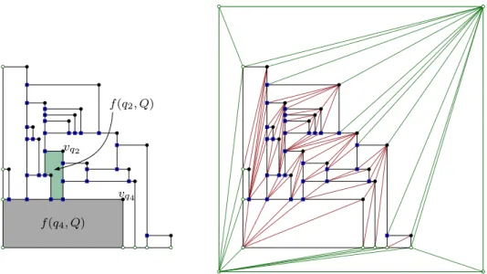
Figure 4The graphsG(Q) (left) andT(Q) (right).
One obstacle is that subproblems should be really independent because we do not want to double count some covered parts. Essentially, a separator in the graph-theory sense does not imply independent subproblems in our context. Another technicality is that some of the subproblems that we encounter recursively cannot be solved optimally; we can only get a lower bound to the optimal value. However, for the subproblems that define the optimal solution at the higher level of the recursion, we do compute an optimal solution.
Let P be a set ofnpoints in the positive quadrant ofR3. Through our discussion, we
will assume thatP is fixed and thus drop the dependency onP andnfrom the notation. We can assume that no point ofP is dominated by another point ofP. Using an infinitesimal perturbation of the points, we can assume that all points have all coordinates different. Let M be the largestx- ory-coordinate inP, thusM = max{px, py |p∈P}. We defineσto be
the square inR2 defined by [−1, M+ 1]×[−1, M+ 1]. It has side lengthM + 2.
For each subsetQofP, consider the projection ofU(Q) onto thexy-plane. This defines a plane graph, which we denote byG(Q); see Figure 4, left. We considerG(Q) as a geometric, embedded graph where each vertex is a point and each edge is a horizontal or vertical straight-line segment on thexy-plane. The projection of each point q∈Qdefines a vertex, which we denote byvq. Each vertexq∈Qdefines a bounded facef(q, Q) inG(Q). This is the
projection of the face on the boundary ofU(Q) contained in the plane{(x, y, z)∈R3|z=qz}.
In fact, each bounded face ofG(Q) isf(q, Q) for some q∈Q. We triangulate each bounded facef(q, Q) ofG(Q)canonically, see Figure 4 right. We add all possible edges from the top rightmost vertexvq, then all possible edges from the bottom leftmost vertex, and finally
all edges from the left bottom-most vertex. This is the canonical triangulation of the face f(q, Q), and we apply it to each bounded face ofG(Q). The outer face ofG(Q) may also have many vertices. We place on top the squareσ, with vertices{−1, M+ 1}2, and triangulate in
some systematic way. LetT(Q) be the resulting geometric, embedded graph, see Figure 4, right. The graphT(Q) is a triangulation of the squareσwith internal vertices. It is easy to see thatG(Q) andT(Q) have O(|Q|) vertices and edges.
We are going to use dynamic programming based on planar separators ofT(Q∗) for an optimal solutionQ∗. Avalid tupleto define a subproblem is a tuple (S, D, `), whereS⊂P, Dis anS-compliant polygonal domain, and`is a positive integer. The tuple (S, D, `) models a subproblem where the points ofS are already selected to be part of the feasible solution, Dis aS-compliant domain so that we only care about the volume inside the cylinderD×R, and we can still select`points fromP∩(D×R). We have two different values associated to
each valid tuple, depending on which subsetsQof vertices from P∩D can be selected:
Φfree(S, D, `) = max{vol(U(S∪Q)∩(D×R))|Q⊂P∩(D×R), |Q| ≤`}.
Φcomp(S, D, `) = max{vol(U(S∪Q)∩(D×R))|Q⊂P∩(D×R), |Q| ≤`,
D is (S∪Q)-compliant}.
Obviously, for all valid tuples (S, D, `) we have Φcomp(S, D, `) ≤ Φfree(S, D, `). On the
other hand, we are interested in the valid tuple (∅, σ, k), for which we have Φfree(∅, σ, k) =
Φcomp(∅, σ, k).
We would like to get a recursive formula for Φfree(S, D, `) or Φcomp(S, D, `) using planar
separators. More precisely, we would like to use a separator inT(S∪Q∗) for an optimal solution, and then branch on all possible such separators. However, none of the two definitions seem good enough for this. If we would use Φfree(S, D, `), then we divide into domains that
may have too much freedom and the interaction between subproblems gets complex. If we would use Φcomp(S, D, `), then merging the problems becomes an issue. Thus, we take a
mixed route where we argue that, for the valid tuples that are relevant for finding the optimal solution, we actually have Φfree= Φcomp.
Avalid partitionπof (S, D, `) is a collection of valid tuplesπ={(S1, D1, `1), . . . ,(St, Dt, `t)}
such that
S1=· · ·=St=S∪S0 for some setS0⊂P∩D; |S0|=Op|S|+`;
the domainsD1,. . .,Dt have pairwise disjoint interiors andD=SiDi;
`=|S0|+P
i`i; and
`i≤2`/3 for eachi= 1, . . . , t.
Let Π(S, D, `) be the family of valid partitions for the tuple (S, D, `). We remark that different valid partitions may have different cardinality.
ILemma 4.1. For each valid tuple(S, D, `)we have
Φfree(S, D, `) ≥ max
π∈Π(S,D,`)
X
(S0,D0,`0)∈π
Φfree(S0, D0, `0),
Φcomp(S, D, `) ≤ max
π∈Π(S,D,`)
X
(S0,D0,`0)∈π
Φcomp(S0, D0, `0).
Proof Sketch. For the first inequality, we show that, for eachπ∈Π(S, D, `), joining solutions to the subproblems Φfree(·) defined by{(S0, D0, `0)|(S0, D0, `0)∈π}gives a feasible solution
for the problem Φfree(S, D, `).
For the second inequality, we consider an optimal solutionQ∗⊆P∩Dwith at most `
points for the problem Φcomp(S, D, `). The triangulationT(S∪Q∗) is a 3-connected planar
cycle separator we can build a valid partitionπγ ∈Π(S, D, `) such thatQ∗∩D0 is a feasible
solution to each (S0, D0, `0)∈πγ. For the correctness argument, we use an easy monotonicity
property of beingQ-compliant, which we skip in this short version. We then have
Φcomp(S, D, `) ≤
X
(S0,D0,`0)∈π
γ
Φcomp(S0, D0, `0),
and the second inequality follows. J
Our dynamic programming algorithm closely follows the inequalities of Lemma 4.1. Specifically, we define for each valid tuple (S, D, `) the value
Ψcomp(S, D, `) =
Φcomp(S, D, `) if`≤O(
√ k);
max
π∈Π(S,D,`)
X
(S0,D0,`0)∈π
Ψcomp(S0, D0, `0), otherwise.
Standard induction on` using Lemma 4.1 implies the following property.
ILemma 4.2. For each valid tuple(S, D, `)we have
Φcomp(S, D, `) ≤ Ψcomp(S, D, `) ≤ Φfree(S, D, `).
Since we know that Φfree(∅, σ, k) = Φcomp(∅, σ, k), Lemma 4.2 implies that Ψcomp(∅, σ, k) =
Φfree(∅, σ, k). Hence, it suffices to compute Ψcomp(∅, σ, k) using its recursive definition. In
the remainder, we bound the running time of this algorithm.
ITheorem 4.3. In 3 dimensions,Volume Selectioncan be solved in time nO(√k). Proof Sketch. We compute Ψcomp(∅, σ, k) using its recursive definition. The base cases,
where` =O(√k), can be solved in nO(`) =nO(√k) time using simple enumeration of all
size-` subsets.
Starting with (S1, D1, `1) = (∅, σ, k), consider a sequence of valid tuples (S1, D1, `1),
(S2, D2, `2), . . . such that, fori≥2, the tuple (Si, Di, `i) appears in some valid partition
of (Si−1, Di−1, `i−1). By the properties of valid partitions, we have `i ≤ 2`i−1/3 and |Si−1| ≤ |Si| ≤ |Si−1|+O(
p
|Si|+`i−1). It follows that the sequence `1, `2, . . . decreases
geometrically, from which one can deduce that|Si|=O(
√
k) for alli. This means that there arenO(√k) valid tuples (S, D, `) that appear in the recursive calls. The same bound can be
shown for the number of valid partitions in each step. J
We only described an algorithm that computesVolSel(P, k), i.e., the maximal volume realized by any size-k subset of P. It is easy to augment the algorithm with appropriate bookkeeping to also compute an actual optimal subset.
5
Efficient Polynomial-time Approximation Scheme
In this section we design an approximation algorithm forVolume Selection.
ITheorem 5.1. Given a point setP of size nin Rd>0, 0≤k≤n, and0< ε≤1/2, we can compute a(1±ε)-approximation ofVolSel(P, k)in timeO(n·ε−d(logn+k+2O(ε−2log 1/ε)d)). We can also compute a set S⊆P of size at mostk such thatµ(S)is a(1−ε)-approximation
The approach is based on the shifting technique of Hochbaum and Maass [21]. However, there are some non-standard aspects in our application. It is impossible to break the problem into independent subproblems because all the anchored boxes intersect around the origin. We instead break the input into subproblems that arealmost independent. To achieve this, we use an exponential grid, instead of the usual regular grid with equal-size cells. Alternatively, this could be interpreted as using a regular grid in a log-log plot of the input points.
Throughout this section we need two numbersλ, τ≈d/ε. Specifically, we defineτ as the smallest integer larger thand/ε, andλas the smallest power of (1−ε)−1/d larger thand/ε. We consider a partitioning of the positive quadrantRd>0into regionsof the form
R(¯x) :=
d
Y
i=1
[λxi, λxi+1) for x¯= (x
1, . . . , xd)∈Zd.
On top of this partitioning we consider a grid, where each grid cell contains (τ−1)d regions
and the grid boundaries are thick, i.e., two grid cells do not touch but have a region in between. More precisely, for any offset ¯`= (`1, . . . , `d)∈Zd, we define the gridcells
C¯`(¯y) := d
Y
i=1
[λτ·yi+`i+1, λτ(yi+1)+`i) for y¯= (y
1, . . . , yd)∈Zd.
Note that each grid cell indeed consists of (τ−1)d regions, and the space not contained in any grid cell (i.e., the grid boundaries) consists of all regionsR(¯x) with xi≡`i (modτ) for
some1≤i≤d.
5.1
Description of the algorithm
Our approximation algorithm works as follows.
(1) Iterate over all grid offsets ¯`∈[τ]d. This is the key step of the shifting technique [21].
(2) For any choice of the offset ¯`, remove all points not contained in any grid cell, i.e., remove points contained in the thick grid boundaries. Call the remaining pointsP0 ⊆P.
(3) The grid cells now induce a partitioning ofP0 into setsP10, . . . , Pm0 , where eachPi0 is the intersection ofP0 with a grid cellCi (withCi =C`¯(¯y(i)) for some ¯y(i)∈Zd). Note that
these grid cell subproblemsP10, . . . , Pm0 are not independent, since any two boxes have a common intersection near the origin, no matter how different their coordinates are. However, as shown below treatingP10, . . . , Pm0 as independent subproblems still yields an approximation.
(4) We discretize by rounding down all coordinates of all points inP10, . . . , Pm0 to powers of3 (1−ε)1/d. We can remove duplicate points that are rounded to the same coordinates.
This yields sets ˜P1, . . . ,P˜m. Note that within each grid cell in any dimension the largest
and smallest coordinate differ by a factor of at most λτ−1. Hence, there are at most
log(1−ε)−1/d(λτ−1) =O(ε−2log 1/ε) different rounded coordinates in each dimension, and
thus the total number of points in each ˜Pi isO(ε−2log 1/ε)d.
(5) Since there are only few points in each ˜Pi, we can precompute allVolume Selection
solutions on each set ˜Pi, i.e., for any 1≤i≤mand any 0≤k0 ≤ |P˜i|we precompute
VolSel( ˜Pi, k0). We do so by exhaustively enumerating all 2|
˜
Pi|subsetsS of ˜P
i, and for
each one computingµ(S) by inclusion-exclusion in timeO(2|S|) (see, e.g., [32, 33]). This
runs in total timeO(m·2O(ε−2log 1/ε)d) =O(n·2O(ε−2log 1/ε)d).
3 Here we use thatλis a power of (1−ε)−1/d, to ensure that rounded points are contained in the same
(6) It remains to split the at mostkpoints that we want to choose over the subproblems ˜
P1, . . . ,P˜m. As we treat these subproblems independently, we compute
V(¯`) := max
k1+...+km≤k
m
X
i=1
VolSel( ˜Pi, ki).
Note that if the subproblems would be independent, then this expression would yield the exact result. We argue below that the subproblems are sufficiently close to being independent that this expression yields a (1−ε)-approximation of VolSel(Sm
i=1P˜i, k).
Observe that the expression V(¯`) can be computed efficiently by dynamic programming, where we compute for eachiandk0 the following value:
T[i, k0] = max
k1+...+ki≤k0
i
X
i0=1
VolSel( ˜Pi0, ki0).
The following rule computes this table:
T[i, k0] = max
0≤κ≤min{k0,|P˜i|} VolSel( ˜Pi, κ) +T[i−1, k 0−κ]
.
(7) Finally, we optimize over the offset ¯`by returning the maximal V(¯`).
In pseudocode, this yields the following procedure:
(1) Iterate over all offsets ¯`= (`1, . . . , `d)∈[τ]d:
(2) P0:=P. Delete anypfrom P0 that is not contained in any grid cellC`¯(¯y). (3) PartitionP0 intoP0
1, . . . , Pm0 , where Pi0 =P0∩Ci for some grid cellCi.
(4) Round down all coordinates to powers of (1−ε)1/d and remove duplicates, obtaining
˜
P1, . . . ,P˜m.
(5) ComputeH[i, k0] :=VolSel( ˜Pi, k0) for all 1≤i≤m, 0≤k0 ≤ |P˜i|.
(6) ComputeV(¯`) := maxk1+...+km≤k
Pm
i=1VolSel( ˜Pi, ki) by dynamic programming.
(7) Return max`¯V(¯`).
5.2
Running Time
Step (1) yields a factor τd =O(1ε)d in the running time. Since we can compute for each point in constant time the grid cell it is contained in, step (2) runs in time O(n). For the partitioning in step (3), we use a dictionary data structure storing all ¯y ∈ Zd with
nonempty P0 ∩C`¯(¯y). Then we can assign any point p ∈ P0 to the other points in its
cell by one lookup in the dictionary, in timeO(logn). Thus, step (3) can be performed in timeO(nlogn). Step (4) immediately works in the same running time. For step (5) we already argued above that it can be performed in timeO n2O(ε−2log 1/ε)d
. Finally, step (6) can be implemented in time O(Pm
i=1|P˜i| ·k) = O(nk). The total running time is thus
O n·ε−d logn+k+ 2O(ε−2log 1/ε)d
.
5.3
Correctness
Combining the following lemmas we show that the above algorithm indeed computes a (1±O(ε))-approximation of VolSel(P).
I Lemma 5.2 (Removing grid boundaries). Let P be a point set and let 0 ≤ k ≤ |P|. Remove all points contained in grid boundaries with offset `¯to obtain the point setP`¯:= P ∩S
¯
y∈ZdC`¯(¯y). Then for all ¯` ∈Z
d we have
VolSel(P¯`, k) ≤ VolSel(P, k), and for
Proof Sketch. Since we only remove points, the first inequality is immediate. For the second inequality we use a probabilistic argument. Consider an optimal solution, i.e., a setS⊆P of size at mostk withµ(S) =VolSel(P, k). LetS`¯:=S∩P`¯. For a uniformly random offset
¯
`∈[τ]d, the probability that a fixed pointp∈S doesnot survive, i.e., we havep6∈S
¯
` is at
mostd/τ ≤ε. Hence,psurvives with probability at least 1−ε.
Now for each pointq∈ U(S) identify a points(q)∈S dominatingq. Sinces(q) survives inS`¯with probability at least 1−ε, the pointqis dominated byS`¯with probability at least
1−ε. By integrating over allq∈ U(S) we thus obtain an expected volume of
E`¯[µ(S`¯)] =
Z
U(S)
Pr[qis dominated byS`¯]dq≥
Z
U(S)
(1−ε)dq= (1−ε)µ(S).
It follows that for some ¯` we have µ(S`¯) ≥ E[µ(S`¯)] ≥ (1−ε)µ(S). For this ¯` we have
VolSel(P`¯, k)≥(1−ε)VolSel(P, k). J ILemma 5.3 (Rounding down coordinates). Let P be a point set, and let P˜ be the same point set after rounding down all coordinates to powers of(1−ε)−1/d. Then for anyk
(1−ε)VolSel(P, k)≤VolSel( ˜P , k)≤VolSel(P, k).
In the proof of the next lemma it becomes important that we have used the thick grid boundaries, with a separating region, when defining the grid cells.
ILemma 5.4 (Treating subproblems as independent I). For any offset`¯, letS1, . . . , Sm be
point sets contained in different grid cells with respect to offset`¯. Then we have
(1−ε)
m
X
i=1
µ(Si)≤µ
[m i=1 Si ≤ m X i=1 µ(Si).
Proof Sketch. The second inequality is the union bound applied toU(S1), . . . ,U(Sm).
For the first inequality, we can decomposeSm
i=1U(Si) to get
µ m [ i=1 Si = vol m [ i=1 U(Si)
! = m X i=1
µ(Si)−vol
U(Si)∩
[
j<i
U(Sj)
. (1)
Now letC`¯(¯y(i)) be the grid cell containingPifor 1≤i≤m, where ¯y(i)= (y
(i) 1 , . . . , y
(i)
d )∈
Zd. We may assume that these cells are ordered in non-decreasing order ofy(1i)+. . .+y (i)
d .
Observe that in this ordering, for anyj < iwe havey(tj)< yt(i)forsome1≤t≤d. Recall thatC`¯(¯y) =Qtd=1[λτ·yt+`t+1, λτ(yt+1)+`t). It follows that each point inSj<iU(Sj) hast-th
coordinate at mostδt:=λτ·yt+`t for some 1≤t ≤d. SettingDt:={(z1, . . . , zd)∈Rd≥0 | zt≤δt}, we thus have Sj<iU(Sj)⊆S
d
t=1Dt, which yields
vol
U(Si)∩
[
j<i
U(Sj)
≤volU(Si)∩ d [ t=1 Dt ≤ d X t=1
vol U(Si)∩Dt
. (2)
LetAbe the (d−1)-dimensional volume of the intersection of U(Si) with the planext= 0.
Since all points in Si have t-th coordinate at least λτ·yt+`t+1 = λ·δt, we have µ(Si) ≥
A·λ·δt. Moreover, U(Si)∩Dt has d-dimensional volume A·δt. Together, this yields
vol(U(Si)∩Dt)≤µ(Si)/λ. With (1) and (2), and using that λ≥d/ε, we thus obtain
µ m [ i=1 Si ≥ m X i=1
µ(Si)−d·µ(Si)/λ≥(1−ε) m
X
i=1
Leveraging the above lemma to VolSelyields the following.
ILemma 5.5(Treating subproblems as independent II). For any offset `¯, letP1, . . . , Pm be
point sets contained in different grid cells, andk≥0. Then we have
(1−ε)· max
k1+...+km≤k
m
X
i=1
VolSel(Pi, ki)≤VolSel(P, k)≤ max k1+...+km≤k
m
X
i=1
VolSel(Pi, ki).
Note that the above lemmas indeed prove that the algorithm returns a (1±O(ε ))-approximation to the valueVolSel(P, k). In step (2) we delete the points containing the the grid boundaries, which yields an approximation for some choice of the offset ¯`by Lemma 5.2. As we iterate over all possible choices for ¯`and maximize over the resulting volume, we obtain an approximation. In step (4) we round down coordinates, which yields an approximation by Lemma 5.3. Finally, in step (6) we solve the problem maxk1+...+km≤k
Pm
i=1VolSel( ˜Pi, ki),
which yields an approximation toVolSel(Sm
i=1P˜i, k) by Lemma 5.5. All other steps do not
change the point set or the considered problem.
5.4
Computing an Output Set
The above algorithm, as described, only gives an approximation for the valueVolSel(P, k). However, by tracing the dynamic programming table we can reconstruct a subsetS ofP of size at mostkyielding a (1−O(ε))-approximation of the optimal volumeVolSel(P, k).
Note that we do not compute the exact volume µ(S) of the output setS. Instead, the valueV(¯`) only is a (1 +O(ε))-approximation of µ(S). To explain this effect, recall that exactly computingµ(T) for any given set T takes timenΘ(d)(under the Exponential Time
Hypothesis). As our running time isO(n2) for any constantd, ε, we cannot expect to compute µ(S) exactly.
6
Conclusions
We considered the volume selection problem, where we are givennpoints inRd>0and want
to selectkof them that maximize the volume of the union of the spanned anchored boxes. We show: (1) Volume selection is NP-hard in dimension d= 2 (previously this was only known when dis part of the input). (2) In 3 dimensions, we design an nO(√k) algorithm
(the previously best was Ω nk
). (3) We design an efficient polynomial time approximation scheme for any constant dimensiond(previously only a (1−1/e)-approximation was known). We leave open to improve our NP-hardness result to a matching lower bound under the Exponential Time Hypothesis, e.g., to show that ind= 3 any algorithm takes timenΩ(√k)
and in any constant dimensiond≥4 any algorithm takes timenΩ(k). Alternatively, there could be a faster algorithm, e.g., in timenO(k1−1/d). Finally, we leave open to figure out the
optimal dependence onn, k, d, εof a (1−ε)-approximation algorithm.
Moving away from the applications, one could also study volume selection on general axis-aligned boxes in Rd, i.e., not necessarily anchored boxes. This problem General Volume Selection is an optimization variant of Klee’s measure problem and thus might
be theoretically motivated. However, General Volume Selection is probably much harder than the restriction to anchored boxes, by analogies to the problem of computing an independent set of boxes, which is not known to have a PTAS [1]. In particular,General
Volume Selectionis NP-hard already in 2 dimensions, which follows from NP-hardness of
Acknowledgements. This work was initiated during the Fixed-Parameter Computational Geometry Workshop at the Lorentz Center, 2016. We are grateful to the other participants of the workshop and the Lorentz Center for their support. We are especially grateful to Günter Rote for several discussions and related work.
References
1 A. Adamaszek and A. Wiese. Approximation schemes for maximum weight independent set of rectangles. InProc. of the 54th IEEE Symp. on Found. of Comp. Science (FOCS), pages 400–409. IEEE, 2013.
2 A. Auger, J. Bader, D. Brockhoff, and E. Zitzler. Investigating and exploiting the bias of the weighted hypervolume to articulate user preferences. InProc. of the 11th Conf. on Genetic and Evolutionary Computation, pages 563–570. ACM, 2009.
3 A. Auger, J. Bader, D. Brockhoff, and E. Zitzler. Hypervolume-based multiobjective opti-mization: Theoretical foundations and practical implications. Theoretical Comp. Science, 425:75–103, 2012.
4 J. Bader. Hypervolume-based search for multiobjective optimization: theory and methods. PhD thesis, ETH Zurich, Zurich, Switzerland, 1993.
5 F. Barahona. On the computational complexity of Ising spin glass models. J. of Physics A: Mathematical and General, 15(10):3241, 1982.
6 N. Beume, C. M. Fonseca, M. López-Ibáñez, L. Paquete, and J. Vahrenhold. On the com-plexity of computing the hypervolume indicator. IEEE Trans. on Evolutionary Computa-tion, 13(5):1075–1082, 2009.
7 N. Beume, B. Naujoks, and M. Emmerich. SMS-EMOA: Multiobjective selection based on dominated hypervolume. European J. of Operational Research, 181(3):1653–1669, 2007.
8 K. Bringmann. Bringing order to special cases of Klee’s measure problem. InInt. Symp. on Mathematical Foundations of Comp. Science, pages 207–218. Springer, 2013.
9 K. Bringmann and T. Friedrich. Approximating the volume of unions and intersections of high-dimensional geometric objects. Computational Geometry, 43(6):601–610, 2010.
10 K. Bringmann and T. Friedrich. An efficient algorithm for computing hypervolume contri-butions. Evolutionary Computation, 18(3):383–402, 2010.
11 K. Bringmann and T. Friedrich. Approximating the least hypervolume contributor: NP-hard in general, but fast in practice. Theoretical Comp. Science, 425:104–116, 2012.
12 K. Bringmann, T. Friedrich, and P. Klitzke. Generic postprocessing via subset selection for hypervolume and epsilon-indicator. InInt. Conf. on Parallel Problem Solving from Nature, pages 518–527. Springer, 2014.
13 K. Bringmann, T. Friedrich, and P. Klitzke. Two-dimensional subset selection for hyper-volume and epsilon-indicator. In Proc. of the 2014 Conf. on Genetic and Evolutionary Comput., pages 589–596. ACM, 2014.
14 T. M. Chan. A (slightly) faster algorithm for Klee’s measure problem. Computational Geometry, 43(3):243–250, 2010.
15 T. M. Chan. Klee’s measure problem made easy. In Proc. of the 54th IEEE Symp. on Found. of Comp. Science (FOCS), pages 410–419. IEEE, 2013.
16 J. Chen, X. Huang, I. A. Kanj, and G. Xia. Linear FPT reductions and computational lower bounds. InProc. of the 36th ACM Symp. on Theory of Computing (STOC), pages 212–221. ACM, 2004.
17 M. Emmerich, A. H. Deutz, and I. Yevseyeva. A Bayesian approach to portfolio selection in multicriteria group decision making. Procedia Comp. Science, 64:993–1000, 2015.
19 M. R. Garey and D. S. Johnson. The rectilinear Steiner tree problem in NP complete.SIAM J. of Applied Math., 32:826–834, 1977.
20 A. P. Guerreiro, C. M. Fonseca, and L. Paquete. Greedy hypervolume subset selection in low dimensions. Evolutionary Computation, 24(3):521–544, 2016.
21 D. S. Hochbaum and W. Maass. Approximation schemes for covering and packing problems in image processing and VLSI. J. ACM, 32(1):130–136, 1985.
22 H. Imai and T. Asano. Finding the connected components and a maximum clique of an intersection graph of rectangles in the plane. J. of Algorithms, 4(4):310–323, 1983.
23 J. D. Knowles, D. W. Corne, and M. Fleischer. Bounded archiving using the Lebesgue measure. In Proc. of the 2003 Congress on Evolutionary Computation (CEC), volume 4, pages 2490–2497. IEEE, 2003.
24 T. Kuhn, C. M. Fonseca, L. Paquete, S. Ruzika, M. M. Duarte, and J. R. Figueira. Hy-pervolume subset selection in two dimensions: Formulations and algorithms. Evolutionary Computation, 2015.
25 G. L. Miller. Finding small simple cycle separators for 2-connected planar graphs. J. Comput. Syst. Sci., 32(3):265–279, 1986.
26 J. S. B. Mitchell and M. Sharir. New results on shortest paths in three dimensions. InProc. of the 20th ACM Symp. on Computational Geometry, pages 124–133, 2004.
27 G. L. Nemhauser, L. A. Wolsey, and M. L. Fisher. An analysis of approximations for maxi-mizing submodular set functions – I. Mathematical Programming, 14(1):265–294, 1978.
28 G. Rote, K. Buchin, K. Bringmann, S. Cabello, and M. Emmerich. Selectingkpoints that maximize the convex hull volume (extended abstract). InJCDCG3 2016; The 19th Japan Conf. on Discrete and Computational Geometry, Graphs, and Games, pages 58–60, 9 2016. http://www.jcdcgg.u-tokai.ac.jp/JCDCG3_abstracts.pdf.
29 J. A. Storer. On minimal-node-cost planar embeddings. Networks, 14(2):181–212, 1984.
30 R. Tamassia and I. G. Tollis. Planar grid embedding in linear time.IEEE Trans. on Circuits and Systems, 36(9):1230–1234, 1989.
31 T. Ulrich and L. Thiele. Bounding the effectiveness of hypervolume-based (µ+λ)-archiving algorithms. InLearning and Intelligent Optimization, pages 235–249. Springer, 2012.
32 L. While, P. Hingston, L. Barone, and S. Huband. A faster algorithm for calculating hypervolume. IEEE Trans. on Evolutionary Computation, 10(1):29–38, 2006.
33 J. Wu and S. Azarm. Metrics for quality assessment of a multiobjective design optimization solution set. J. of Mechanical Design, 123(1):18–25, 2001.