Missing Data in Non-parameteric Tests of Correlated Data

(1)

MISSING DATA IN NON-PARAMETRIC TESTS

OF CORRELATED DATA

Annie Green Howard

A dissertation submitted to the faculty of the University of North Carolina at Chapel Hill in partial fulfillment of the requirements for the degree of Doctor of Philosophy in the Department of Biostatistics.

Chapel Hill 2012

Approved by:

Shrikant Bangdiwala Lloyd J. Edwards Gerardo Heiss Gary Koch Paul Stewart

(2)

c

2012

(3)

Abstract

ANNIE GREEN HOWARD: MISSING DATA IN NON-PARAMETRIC TESTS OF CORRELATED DATA

(Under the direction of Shrikant Bangdiwala)

Many public health studies are designed to test for differences in repeated

measure-ments. Measurements on the same subject are not independent and therefore analysis

methods must take correlation into account. A number of tests have been developed to

analyze this type of data. Two prominent non-parametric methods, used often when

one is not willing to make any distributional assumptions about the data, include

Fried-man’s test and a variation on FriedFried-man’s test proposed by Koch and Sen that requires

no assumptions to be made about the correlation between measurements.

While both tests require complete and balanced data, in many studies missing data

can arise for a variety of reasons. Researchers have developed a number of methods

to adapt Friedman’s test to situations involving missing data when it can be assumed

that the missing data are missing completely at random. We propose applying these

same adjustments to the test statistic proposed by Koch and Sen to adapt this test to

deal with data that are missing completely at random. This method involves using the

sum of the reduced ranks, rather than the average rank, across all subjects to allow

for meaningful comparisons across subjects. An inflation factor is used to ensure the

missing data do not result in a substantial loss of power.

The assumption that the data are missing completely at random is often too strict

(4)

di-Friedman’s test and Koch and Sen’s test to informative missing data scenarios. The

method put forth in this paper involves the use of single imputation to impute missing

rank values along with a weighting scheme which assigns smaller weight to individuals

with more missing data. Guidelines and suggestions are put forward as to when this

new method would be preferred to the method currently used to address problems with

(5)

Acknowledgments

I wish to thank Dr. Shrikant Bangdiwala for his insight, encouragement and

friend-ship throughout this process. His confidence in my skills along with his guidance and

support have helped me to make it through both the ups and downs of this process.

Dr. Gary Koch has also been instrumental in the development in this research and I

would like to thank him for his input and ideas. I would also like to acknowledge Dr.

Lloyd Edwards, Dr. Gerardo Heiss, Dr. Paul Stewart and Dr. Stephan Weiland who

have offered many helpful suggestions and ideas that went into this dissertation.

I could not have completed this without the love and support of my family. In

particular, Id like to acknowledge my father Dr. George Howard who offered advice

and assistance at every stage of the process. His belief in me has and will continue to

be instrumental in my future success. I’d also like to thank my mother, Dr. Virginia

Howard, for the countless words of encouragement and support. In addition she has

lived her life in such a way that her career has served to help me in the development of

my personal and professional goals. My sisters, Marjorie Howard and Letitia Perdue

have offered nothing but unconditional love and support which has been invaluable

during this process.

I cannot thank enough the staff, faculty and students at UNC, particularly within

the Biostatistics Department. This has been a difficult but rewarding process and the

generosity, patience, acceptance and assistance of the friends I have made within this

(6)

Melissa Hobgood, Virginia Pate, Allison Deal and my fellow members both official and

unofficial of The Cave. I would also like to thank specifically the CSCC for their

flexi-bility and financial support. This work was supported in large part by Training Grant

(7)

List of Tables

1.1 Repeated Measures Data Set with Missing Data . . . 6

1.2 Non-Parametric Test With Complete and Balanced Data . . . 8

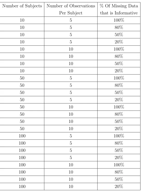
2.1 Data Sets Generated . . . 42

A.1 Type I Error Rates . . . 120

A.2 Power Under a Linear Increase of 0.25 . . . 121

A.3 Power Under a Linear Increase of 1 . . . 122

A.4 Average Pain Scores By Period of the Day for IBS Study . . . 123

B.1 Type I Error Rates . . . 127

B.2 Power Under a Linear Increase of 0.25 . . . 128

B.3 Power Under the Alternative of a Linear Increase of 0.5 . . . 129

B.4 Complete Ranking of 4 Objects by 20 Subjects . . . 130

B.5 Ranking of 4 Objects by 20 Subjects with Missing Data . . . 131

C.1 Type I Error Rates - 10 Subjects . . . 137

C.4 Power Under a Linear Increase of 0.25 - 10 Subjects . . . 140

(13)

C.6 Power Under a Linear Increase of 0.25 - 100 Subjects . . . 142

C.7 Power Under a Linear Increase of 1 - 10 Subjects . . . 143

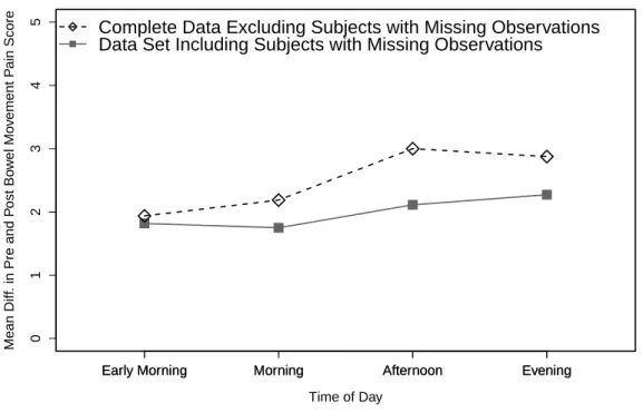
C.10 Avg. Difference in BM Pain Scores By Period of Day . . . 146

(14)

List of Figures

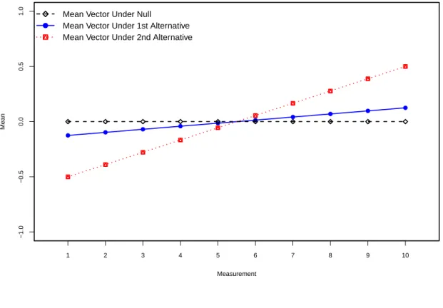
2.1 Mean Vectors for Null and Alternative Hypotheses . . . 43

2.2 Type I Error Rates . . . 44

2.3 Power (Under Linear Increase of 0.25) . . . 45

2.4 Power (Under a Linear Increase of 1) . . . 46

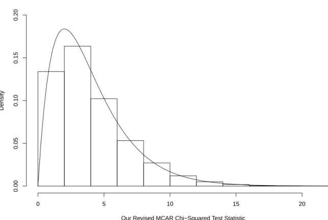
2.5 Asymptotic Behavior of Our Revised Test Statistic . . . 47

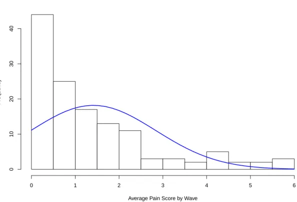
2.6 Histogram of Average Pain Score by Wave with Normal Curve . . . 49

2.7 Average Pain Score by Period of Day . . . 50

3.2 Type I Error Rates by % Informative Missing - 10 Subjects . . . 71

3.3 Type I Error Rates by % Informative Missing - 50 Subjects . . . 72

3.4 Power by % Informative Missing (Increase of 0.25) - 10 Subjects . . . . 73

3.9 Mean Rank for Each Object . . . 78

4.2 Type I Error Rate by % Informative Missing - 10 Subjects . . . 96

(15)

4.4 Type I Error Rate by % Informative Missing- 100 Subjects . . . 98

4.7 Power by % Informative Missing (Increase of 0.25) - 100 Subjects . . . 101

4.8 Power by % Informative Missing (Increase of 1) - 10 Subjects . . . 102

(16)

Chapter 1 Introduction and Literature Review

1.1 Introduction

1.1.1 Motivation

Many public health studies are designed to test for a difference between repeated

measurements on the same subject. These studies can be useful in a number of different

contexts including, but not limited to, testing the reliability of a particular procedure

using repeated measurements on the same individuals, testing for a change in average

values or proportions over time, and testing for an effect of different treatments on the

same subject over a follow-up period. In all of these cases, measurements on the same

subject are not independent and therefore analysis methods must take into account

the correlation between measurements taken on the same subject. Recently, some of

the analytic approaches for this type of data analysis have been generalized to account

for missing data. In large sample studies, these methods have been proven to produce

accurate type I error rates in certain scenarios although the preferred analysis method

differs depending on a number of factors.

Non-parametric methods are one of the approaches for which these adaptations

(17)

only been developed for scenarios where one can assume the correlation between any

two measurements on the same subject is the same. This is problematic for many

repeated measures studies, particularly longitudinal studies, when one can often make

the assumption that the correlation between two measurements that are close together

in time are likely to be more strongly correlated than measurements farther apart in

time.

These non-parametric adjustments that seek to minimize bias and preserve the

ac-curacy of type I error rates have been proven to be effective only when the probability

an observation is missing does not depend on the outcome or covariate values,

com-monly referred to as missing completely at random (MCAR). Some researchers have

investigated the power of these adjusted tests, finding the reduction in power not to be

an of great concern in the case of MCAR data (Kenward and Roger, 1997; Schluchter

and Elashoff, 1990; Catellier and Muller, 2000; Manor and Zucker, 2004; Kawaguchi

and Koch, 2010).

In practice the reasons for missingness, if even known, can be complex and

assum-ing MCAR can potentially lead to accuracy problems when testassum-ing hypotheses. Often

in studies involving repeated measurements, missingness is informative, meaning

miss-ingness depends on the actual outcome values themselves. Current methods have not

been adapted to deal with this missingness scenario and there is a strong potential for

biased results when attempting to make inference when incorrectly assuming that the

data are MCAR.

1.1.2 Example

The first example this research will address is a longitudinal study testing for a

(18)

the same number of measurements planned to be recorded for each subject. A

contin-uous outcome is to be measured at each of these time points. Measurements closer in

time tend to be more highly correlated than measurements further apart in time and

therefore equal correlation between any two measurements is highly unlikely.

Specif-ically we will be looking at a study in which investigators were interested in testing

if pain scores differed throughout a day. Participants with irritable bowel syndrome

(IBS) were asked to record pain scores (on a scale from 0 to 10) at wake up, morning,

midday, evening and bedtime. Measurements were collected over a large number of

days and so pain scores were collapsed by averaging pain scores for each period of the

day across all days. Occasionally patients forgot to record pain scores. If the pain score

was missing for more than 40% of all days for a particular period the average pain score

for that subject at that period of the day was set to missing. In the larger context,

it is important to note that missing data occur in longitudinal studies in a number of

contexts. In this case, it is reasonable to assume the chance of a subject reporting a

missing value is unrelated to the outcome value.

The second example involves a situation where a number of judges were each asked

to rank a number of objects. In this scenario, since the objects are naturally ranked,

non-parametric methods are a natural choice of analysis. Researchers are interested in

testing for a preference in objects. Therefore, one is interested in testing if the rank

for each object is the same, although differences between judges are not of interest.

In this scenario, some judges felt uncomfortable ranking one or more of the objects.

This could happen when one object was noticeably better or worse than the remaining

objects. Therefore, one would expect that these missing ranks were more likely to be

higher ranks. This scenario would be similar to one in which lab measurements were

collected on the same subject at one clinic visit and researchers tested for a within

(19)

were taken at the same time, to be highly correlated. In the case of a particular lab

outcome, we assume that the results from each aliquot, coming from the same subject,

will be equally correlated with all other aliquots. Some loss of data is expected in this

study as some aliquots were lost or broken during the transportation of the samples to

the lab. In addition with this data set, the lab equipment cannot measure certain lab

values when values fall outside of a pre-specified value, in the case of this study when

the lab values are extremely high.

The final example examined in this research involves a similar situation to that

described in the first example. Researchers were interested in testing to determine if

there was a difference in the difference in pre and post-bowel movement pain scores

throughout the day. Subjects suffering from irritable bowel syndrome (IBS) were asked

to rank pain on a scale from 0 to 10 before and after every bowel movement. Based

on the time stamp of these measurements, the difference in pre and post-bowel pain

scores were classified as early morning, morning, afternoon or evening. This study

en-rolled both diarrhea predominant (IBS-D) and constipation predominant IBS (IBS-C)

patients. IBS-C patients were more likely to have missing data when they were

ex-periencing IBS symptoms. A missing value for these participants was often indicative

of a higher pre-bowel pain score as they were experiencing constipation. As such, one

expects missing measurements to be higher than the non-missing counterparts. A

sim-ilar situation can develop in any longitudinal trial with missing data. While subjects

may miss a visit randomly, some also drop out of studies due to a change in location or

health status. If a patient drops out of the study due to health status, this can be due

to either the participant’s health improving or declining to a point that they are no

longer interested or able to participate in the study. These improvements or declines

can be associated with better or worse outcome values, often denotes by extremely high

(20)

1.2 Literature Review

1.2.1 Notation and Assumptions

We will generalize this research to a study designed with n planned measurements

recorded for each of the k subjects. We denote the jth _{measurement for the} _ith

indi-vidual as the scalar Yij and Xij denotes any additional covariates collected on the ith

subject along with thejth _{outcome measurement. These} _X

ij values can either vary by

measurement or can be constant within a subject. For our research, we will assume all

covariates are constant within a subject and therefore that Xij =Xi for all i.

Missing outcome values occur often in repeated measures studies. Any scenario

involving missing data also involves a loss of information and therefore analysis with

missing data will often differ from the analysis of the data if it was a complete data

set. Missing data is a very common occurrence and one that must be accounted for in

order to minimize bias and loss of efficiency both of which are associated with missing

data. To classify missingness, a variable Rij is specified as an indicator variable to

denote if Yij is missing. Rij takes the value of 1 if the Yijth observation is observed

and 0 otherwise. Table 1.1 below illustrates that all the information gathered can be

summarized by reporting these three values (Yij, Xij, andRij).

The notation Yi will denote the full vector of missing and observed responses for

the ith _{subject (Y}

i1, Yi2, . . .Yin) and the notation Ri will denote the corresponding

vector for the indicators Rij. Each of these vectors has n elements, corresponding to

the n measurements taken on each subject.

1.2.2 Non-parametric Analysis of Complete and Balanced Data

There are a number of situations in which there are problematic and potentially

(21)

Table 1.1: Repeated Measures Data Set with Missing Data

Measurement

Subject 1 2 . . . n

1    Y11 X1 R11       Y12 X1 R12      

Y1n

X1

R1n

   2    Y21 X2 R21       Y22 X2 R22      

Y2n

X2

R2n

   . . . . k   

Yk1

Xk

Rk1

     

Yk2

Xk

Rk2

      Ykn Xk Rkn   

values may be inappropriate. A number of non-parametric approaches to the repeated

measures analysis have been adapted to deal with such scenarios. The earliest methods

focused on data in which each subject had the same number of measurements, known

as balanced data, and data where there were no missing values, known as complete data

(Friedman, 1937; Koch and Sen, 1968). While there are methods to test for differences in

measurement within a subject if the effects are different between subjects, this research

will be focusing on methods that assume the measurement effect is constant across all

subjects.

Within this subset of methods, the preferred method depends on assumptions one

is willing to make. One such assumption involves, what Koch and Sen refer to as, the

additivity of subject effects. When this assumption is true, it is reasonable to believe

that comparisons of between block rankings are meaningful. This involves assuming

that the difference between two ranked measurements on the same subject is comparable

(22)

Sen, 1968; Stokes, Davis and Koch, 2000). If one assumes the additivity of subject

effects, methods take this into account and adapt their methods so rank comparisons

between subjects are used. The most widely accepted class of these testing methods

involves the use of aligned rank tests. The premise behind all these tests is that some

function of the data for the subject, usually a measure of location, is subtracted from

all the Yij values. These differences are then treated as the outcome variables and are

ranked within a subject (Stokes, Davis and Koch, 2000; Hodges and Lehmann, 1962;

Sen, 1968; Lehmann and D’Abrera, 2006; Koch and Sen, 1968).

Friedman’s Test

One of the most widely-used non-parametric methods, Friedman’s test, utilizes

par-tial rank transformation methods to test for the hypothesis of no difference in

measure-ments within a subject while assuming no additivity of subject effects. In studies where

compound symmetry can be assumed, Friedman’s statistic tests the measurement

ef-fect while controlling for any subject efef-fect. This test does not require the normality

assumptions of parametric methods and also minimizes the effect of the between

sub-ject variability, allowing tests to focus on measurement effect (Friedman, 1937; Stokes,

Davis and Koch, 2000).

Friedman’s method assumes that all outcome variables Yij come from an

n-variate continuous cumulative distribution functionFi whereFi =Gi(y−bi+θj). The

focus of this test is in testing for a measurement effect while controlling for subject.

Therefore hypothesis testing involve testing ifθj = 0 for allj, under the constraint that

P

θj = 0. No additional covariates are included in analysis and therefore no Xi’s are

involved in the test statistic.

Friedman’s test replaces the original measurement values by within subject ranks.

(23)

Yij would be replaced with within subject rank, which will be denoted rij where

rij = 1,2, ...ni. For complete and balanced data sets, we assume the total number

of non-missing measurements is the same for all subjects. Thus, for any subject i,

ni =n. It is important to note that Pn_j₌₁rij = n(n₂+1) for all k subjects. The data in

Table 1.1 can be summarized in a new format, which allows for a display of the same

data in a new format show in Table 1.2 below:

Table 1.2: Non-Parametric Test With Complete and Balanced Data

Measurement Subject 1 2 . . . n

1 r11 r12 r1n

2 r21 r22 r2n

. . . . k rk1 rk2 rkn

If there was no difference in measurements collected on the same subject, one would

expect each rank to be equally likely to be located in each of the n columns.

There-fore, under the null hypothesis of no measurement effect, one would expect the mean

rank for each column to come from a distribution with a mean of the average rank,

n+1

2 . The variance of this distribution under the null hypothesis can be calculated to

be n₁₂2−_k1, where k denotes the number of subjects. Friedman’s test statistic, based off these values for the mean and variance, is:

12k n(n+ 1)

n

X

j=1

¯ rj −

1

2(n+ 1)

2

where ¯rj is the average rank of the jth column. In small studies, it is best to use

the exact permutation distribution to test the null hypothesis of no trend across the

columns, or in the case of longitudinal data no trend over time. However, when the

(24)

distribution withn−1 degrees of freedom.

Tied outcome variables can be dealt with by assigning the tied ranks at random

to each of the tied measurements. However, the mid-rank method is a more common

method that allows for the utilization of more information. This method involves giving

tied measurements the average value of the ranks for which two or more observations

are tied (Friedman, 1937).

This method, with the use of the mid-rank option for ties, is equivalent to combining

Kruskal-Wallis tests while conditioning on subject which is equivalent to a stratified

Mantel-Haenszel tests with column scores being equal to within subject ranks. Since

Friedman’s test can only be used in the case of complete and balanced data, in this case

only the stratified Mantel-Haenszel statistic equivalent to Friedman’s statistics. Both

involve tests to determine if mean responses differ using within subject rank scores

rather than actual measurement values (Landis, Heyman and Koch, 1978; Stokes, Davis

and Koch, 2000).

Koch and Sen’s Test

If it is not reasonable to assume a compound symmetric correlation structure, Koch

and Sen have proposed an alternative to Friedman’s test. This method also uses partial

rank transformation and therefore the data structure is identical to that shown in

Ta-ble 1.2. Where the two methods differ is in terms of the permutation-based distribution

under the null hypothesis. In Friedman’s test, when the correlation is equal between

any two measurements within a subject, the distribution of the ranks under the null

hypothesis is based off of the fact that each permutation of ranks is equally likely

within each subject. The distribution used for the test statistic in Koch and Sen’s test

is based off of the premise that when compound symmetry is violated, the unique pair

(25)

and Sen’s test, the distribution under the null hypothesis allows for only two possible

permutations of ranks within a subject. The first possible permutation is the observed

permutation and the second is the exact opposite permutation, specified explicitly

be-low. For both of these permutations the correlation between any two measurements is

the same, thereby preserving the correlation structure (Koch and Sen, 1968).

ri = (ri1, ri2, ..., rin)

ri = (n+ 1−ri1, n+ 1−ri2, ..., n+ 1−rin)

These two permutations for the ith_{subject are the only two permutations that have}

the same correlation as the observed data for theith_{subject. Each of these permutations}

are assumed to be observed with equal probability under the null hypothesis that there

is no difference in measurements within a subject. Koch and Sen’s method tests for a

measurement effect while controlling for subject, and therefore the results are combined

across all subjects to get an estimated average effect across all subjects. Interest lies

in tests involving Twhich is a n x 1 vector with elements Tj = _k1 k

P

i=1

rij.

Under the null hypothesis of this distribution, the expected value of Tj can be

calculated based on the expected value of rij which is equal to n+1₂ .

E[Tj] =

1 k

k

X

i=1

E[rij] =E[rij] = ((rij)P r(rij =rij) + (n+ 1−rij)P r(rij =n+ 1−rij))

= rij

1

2 + (n+ 1−rij) 1 2 =

(26)

Under the assumptions required for Koch and Sen’s test, the covariance matrix of

T, anxn matrix, will be denoted as V with each element vjj0 calculated as:

vjj0 =Cov(T_j, T_j0) = Cov(

1 k

k

X

i=1

rij,

1 k

k

X

i=1

rij0) = 1 k 2 k X i=1

Cov(rij, rij0)

= 1

k2

k

X

i=1

(E[(rij −E[rij])(rij0 −E[r_ij0])])

= 1

k2

k

X

i=1

E[rijrij0]−

n+ 1 2 2! = 1 k2 k X i=1

(rijrij0)

1

2 + (n+ 1−rij)(n+ 1−rij0) 1 2−

n+ 1 2

1₂!

= 1 k2 k X i=1

2rijrij0

2 −

rij(n+ 1)

2 −

rij0(n+ 1)

2 +

(n+ 1)2

2 −

1

2(n+ 1) 2 2 = 1 k2 k X i=1

rijrij0 −

rij(n+ 1)

2 −

rij0(n+ 1)

2 +

n+ 1 2 2! = 1 k2 k X i=1

rij −

(n+ 1)

2 rij0−

(n+ 1) 2

Koch and Sen developed a generalized statistic which allows for the testing of any

linear contrast C of the vectorT, which consists of all n Tj elements, for whichCj =

0 where j0 = (1, ...,1). The form of the generalized statistic is stated in terms of

the contrast matrix as T0C0(CVC0)−1CT. Under the null hypothesis k1/2T is an asymptotically multivariate normal vector of rank n−1. Therefore, the test statistic

T0C0(CVC0)−1CT has an asymptotically chi-squared distribution with n−1 degrees

(27)

1.2.3 Missing Data Mechanisms

Missing Covariates

Although in some studies missing covariates can also be a problem, we will be

assuming no missing covariates in our examples. Background on dealing with missing

covariates is included for completeness since this can present substantial concerns.

Var-ious methods exist to address the problems that arise from missing covariates, but for

simplicity we will deal with studies that have complete covariate data. Missing

covari-ates can potentially be an issue in all types of studies; however, in repeated measures

scenarios it can often have a greater impact on the analysis, as one missing covariate

can affect multiple observations on one participant. One method used to address these

concerns involves replacing the missing covariate with the mean or median value of

the covariate. An alternative method involves replacing the missing value by the

pre-dicted value generated by regressing the covariate with missing values on all observed

covariates. More recently, methods often used for dealing with missing outcome values

have been adapted for use in dealing with missing covariates values, including

max-imum likelihood methods, weighted estimating equations and multiple imputations.

However, these are not directly incorporated into the basic repeated measures

mod-eling procedures in many computer-programming packages, including SAS. These can

be done separately from repeated measures analysis computing procedures, although

they are more computationally intensive, particularly the more complex methods, and

these methods do require additional assumptions. In order to simplify analysis, the

most common method of dealing with missing covariates is that all observations for a

participant are deleted if one or more covariates are missing, which can lead to a much

smaller sample size and to biased estimates unless the covariates are missing

com-pletely at random (Horton and Kleinman, 2007). This research will consider data with

(28)

Missing Completely at Random (MCAR)

When outcome variables are missing completely at random (MCAR), the

proba-bility of a subject having a missing value for an observation does not depend on the

subject’s observed values or the covariates. MCAR data are defined explicitly to be

data in which the indicator vector for missingness, Ri, is independent of both Yi and

Xi. This is equivalent to stating P r(Ri|Yi, Xi) = P r(Ri) (Fitzmaurice, Laird and

Waire, 2004). As a number of analyses require the assumption that missing data are

MCAR, this assumption is often assumed even though it requires the strictest

assump-tions.

In studies with repeated measures over time, participants have a higher

proba-bility of missing later visits due to fatigue or lack of interest as the study continues. In

these studies missing data are often classified at MCAR since missingness depends only

on time, which is often treated as a design variable in the case on longitudinal studies.

Unlike covariates, design variables are specified by the investigator and predetermined

for use in the study design. If time is fixed and treated as a design variable, the

miss-ingness depends on a fixed variable and therefore not on the observed or unobserved

data. Therefore time is not included in the covariate matrix and the missingness is

MCAR (Fitzmaurice, Laird and Waire, 2004).

Covariate Dependent Missingness or Missing at Random (MAR)

Covariate dependent missingness, commonly referred to as missing at random (MAR),

occurs when the probability of a subject having a missing value does not depend on

the actual missing outcome values but could depend on a subject’s covariates. Stated

explicitly, covariate dependent missingness is defined to occur when P r(Ri|Yi, Xi) =

(29)

and is still considered likely in studies involving repeated outcome measurements.

As-suming MCAR requires less strict assumptions and therefore fewer methods of analysis

are valid. Under the assumption of covariate dependent missingness, the distribution of

the data used for analysis, the observed, is not the same as the population of interest.

Therefore, the parameter estimates will be biased when using least squares methods

and will only be accurate with maximum likelihood methods when the distribution of

the outcome is correctly specified (Fitzmaurice, Laird and Waire, 2004).

Non-ignorable or Informative Missingness

As knowing that an observation is missing reveals no information about the

ac-tual missing values, both MCAR and covariate dependent missingness are commonly

referred to as non-informative or ignorable missing data. In these cases knowing the

actual missing values is not needed to conduct valid analyses. In contrast, the third

type of missing data, missing not at random (MNAR), is commonly referred to as

informative or non-ignorable missingness. In this situation P r(Ri|Yi,Xi) cannot be

simplified, meaning the probability of a subject having a missing value depends on the

actual unobserved missing values. In this case, not incorporating information about

the missing data will yield biased results. There is not currently a computationally

simple method when dealing with this type of data for statistical estimation and

test-ing. The most common method, which is extremely difficult to do with great accuracy,

requires specifying models both for the response as well as the missing data mechanism.

This requires definingP r(Ri|Yi, Xi) accurately and explicitly (Fitzmaurice, Laird and

(30)

Monotonic vs. Non-Monotonic Missingness

All three of these categories can be further classified, if the order of the repeated

measures has meaning, by specifying the missing data as monotonic or non-monotonic.

If having a missing value forces all subsequent values for a subject to be missing as

well, the missing mechanism is considered to be monotonic. This is commonly referred

to as drop-out or loss to follow up in longitudinal studies. In contrast, non-monotonic

missing data occur when a measurement can be observed after a missing measurement

was reported for that subject. When missing data are non-monotonic, non-informative

missingness is easier to assume and more likely to be valid. For example, when a subject

drops out it is difficult to assume the reason for drop out is completely unrelated

to the subject’s missing outcome values. In contrast, if a subject has intermittent

missing data, it is easier to assume the missingness is unrelated to the missing outcome

values. Additionally, for subjects with intermittent missingness, the observed data

which occurred after the missing data can help in making assumptions about the true

missing values with greater accuracy (Fitzmaurice, Laird and Waire, 2004).

1.2.4 Missing Data in Repeated Measures Analysis

Complete-Case Analysis

There are a number of methods for dealing with missing data. The simplest

ap-proach is known as complete-case analysis, in which any subject with one or more

observations missing is excluded from the analysis. Only data from subjects who have

no missing data are included in the analysis. Using this method with informative

miss-ing data will result in noticeably biased results. If for example participants with high

values were more likely to drop out of a study, the missingness is informative and any

(31)

only situation in which complete case analysis would produce unbiased analyses would

be MCAR, as that is the only situation in which dropping those with missing data

would be dropping a random sample of the population. However, even with MCAR

data, the decrease in sample size could lead to a substantial decrease in power. With

small samples, the loss of even a small number of observations can have an important

effect. However, due to the ease of analysis and interpretation, complete case analysis

is still considered an option of handling missing data (Fitzmaurice, Laird and Waire,

2004).

Repeated Measures ANOVA

Repeated measures analysis of variance (ANOVA) requires complete and balanced

data and is therefore is often used in conjunction with complete case analysis. This

method assumes the correlation between an individual’s measurements are based on the

individual’s underlying tendencies that remain the same for all measurements. This is

one of the earliest methods developed but due to ease of computation and

interpreta-tion, this method is still commonly used even though it requires making assumptions

that may not always be valid. Repeated measures ANOVA assumes the individual

has a latent response which is the same for all measurements thereby assuming some

individuals tend to have overall higher or lower outcomes than the population. This

method forces the data to have a compound symmetric correlation matrix, meaning

the correlation is the same between any two time points. Compound symmetry is

par-ticularly questionable in longitudinal studies as one would expect measurements taken

further apart in time to have weaker correlation than measurements closer in time

(32)

Single Imputation

An additional approach to handling missing data is imputation, in which each

miss-ing value is replaced by some estimated value. There are many approaches to

impu-tation. The simplest case is that of single imputation, in which the missing value is

replaced with one value generated as an estimate of the true unobserved value. Within

this category, imputation can be broken down further into within individual

imputa-tion, where the estimates are gathered from the individual with the actual missing

value, or between individual imputations, in which information from the entire

sam-ple or a portion of the samsam-ple is used to estimate the missing value for an individual.

Missing values for an individual of a particular subgroup, for example females, may be

imputed to be the overall mean of that particular subgroup. One of the most common

within individual single imputations for monotonic missing data is last observation

carried forward (LOCF), in which a subject’s last known measurement is substituted

for all successive missing values. However, the assumption of a stable outcome after

drop out is unrealistic and the standard errors are smaller than they would be in the

case of non-missing data. A number of other functions of the data, both within the

individual as well as data from the overall sample, can replace the missing data. Some

of the more frequently used values for single imputation include the mean value for

a subject, the baseline value, or a worse or best case value, known as extreme case

analysis (Fitzmaurice, Laird and Waire, 2004).

Multiple Imputation

Single imputation methods do not take into account the variation and uncertainty

of predicting an unobserved value. Multiple imputation methods have been developed

to address this concern. These methods involve replacing the missing value with a

(33)

number of possible values for the missing value, generally somewhere between 3 and

10, are generated (Schafer, 1999). The methods of generating these imputed values

can greatly affect the analyses. All methods rely on using the observed data to predict

the missing data. One of the more common methods involves generating the

imputa-tions from an estimated proper prior distribution generated from the observed data.

For more complex situations, Markov Chain Monte Carlo (MCMC) methods can be

used. Both methods require multivariate normality; however, with minor departures,

accurate inferences can still be made using these estimates (Horton and Lipsitz, 2001).

One complete data set is generated from each one of the generated estimates of

the missing value. The complete data sets created from these multiple estimates of the

missing values are then used to determine parameter estimates and variances. Denoting

the parameter estimate or the combination of parameter estimates as Q, m

imputa-tions would result in m estimates of Q, denoted as Qˆ, with each having a variance

estimator U. These multiple Qˆ estimates are then averaged to create a point

esti-mate for Q. The estimate of the variance of this point estimate incorporates both the

between-imputation and within-imputation variance. In the multivariate case, where

ˆ

Q is a vector of values, the within-imputation varianceU¯ is the average of the m

co-variate matrices U. The between imputation B is _m1₋₁

m

P

t=1

(Qˆt ₋_Q_¯₎₍_Q_ˆt ₋_Q)_¯ T_{. The}

total variance can then be expressed as T = U¯ + (1 +m−1₎_B_{. If we define} _k _{to be}

the number of elements in Q, then inference can be made by comparing the

statis-tic (Q¯−Q0)TT−1(Q¯−Q0)

k to an F distribution with k numerator degrees of freedom and

v = (m −1)(1 +m−1)tr(BT−1)/k −2 denominator degrees of freedom. In multi-variate cases, especially with only a small number of imputations, it becomes more

complicated as the between-imputation covariance matrix would not be of full rank

when the number of imputations is less than or equal to the number of elements in Q.

(34)

Generalized Estimating Equations

Methods have been developed that analyze all observed data without imputing

the missing values or excluding subjects with missing data. One of these methods

involves the use of generalized estimating equations, known also as marginal models,

which extends generalized linear model theory to correlated data. As in generalized

linear models, a link and a variance function are specified that connect the outcome

to a linear combination of covariates. These methods do not require any distributional

assumptions be made about the outcome variable but rely on quasi-likelihood methods

in order to estimate parameters and test hypotheses. Instead of making assumptions

about the distribution of the outcome variable, a correlation structure must specified

(Liang and Zeger, 1986). When dealing with a continuous outcome, which we will be

focusing on in this research, the mean model is defined as

µi =E[Yi|Xi] =Xiβ

The specification of the variance component involves the specification of the

corre-lation structure. The general covariance matrix of Yi is specified as

Vi =φA

1 2

iWi(α)A

1 2

i

where Ai is an ni x ni matrix with the elements consisting of the variance of Yi along

the diagonal. Here Wi is the working correlation matrix; an ni x ni matrix which

is a function of the correlation parameters α. Once these are specified, the equation

below can be solved in order to get parameter estimates, for both mean and covariance

parameters.

k

X

i=1

dµ0_i

(35)

In this equationVidenotes the covariance matrix andµidenotes the estimate of the

mean for the ith individual. Here we note that dµ

0 i

dβ is an s x s matrix where s denotes

the number of mean parameters in the model as β is an s x 1 vector. The estimate

for the covariance matrix is calculated based on the working correlation matrix. The

model-based estimate of the covariance matrix is specified as:

k

X

i=1

dµ0_i dβV

−1

i dµi

dβ !−1

If the working correlation matrix is misspecified, this estimate of the covariance

matrix will be incorrect and the standard errors of the estimates will be inaccurate.

Even when the correlation structure is misspecified and the standard errors are invalid,

the mean parameter estimates are accurate since the mean model is separate from the

covariance model. However, inference about the parameter estimates will be invalid.

As a solution, an empirical estimator, commonly referred to as the sandwich estimator

has been derived and can be a more accurate estimator of the covariance ofYi

k

X

i=1

dˆµ0_i dβ

ˆ

V_i−1dµˆi dβ

!−1 _k

X

i=1

dµˆ0_i dβ

ˆ

V_i−1(Yi−µˆi)(Yi −µˆi) 0

ˆ

V_i−1dµˆi dβ

! _k

X

i=1

dµˆ0_i dβ

ˆ

V_i−1dµˆi dβ

!−1

If the working correlation matrix is relatively accurate, the results can be more

effi-cient than when using the model based estimator. Although there are many advantages

to using generalized estimating equations, including the use of all observed data, these

methods will yield unbiased estimates only in the case of MCAR (Stokes, Davis and

Koch, 2000; Fitzmaurice, Laird and Waire, 2004).

Mixed Models

With recent computing advances, mixed models has become one of the most

(36)

is commonly expressed by the following equation where i= 1,2, ...k:

Yi = Xiβ+Zibi +i

Suppose Yi is the ni x 1 vector of non-missing outcomes for the ith subject andXi

is the fixed effect design matrix containing the covariates of interest. In this model, Zi

is defined as a subset of theXi matrix known as the random effects design matrix. We

define bi as the vector of unobserved random effects for the ith subject and i as the

unobserved vector of within-subject error. In this modelbi and i are assumed to have

multivariate normal distributions and to be independent of each other. We can write

this as follows:

   bi i  

:N

      0 0    ,    σ2 b 0

0 σ2

     

If the Zi matrix is a ni x 1 column of ones, the model is simplified. Based on these

assumptions, the covariance matrix forYi can be defined asP_i = σ_b2110 +σ2I where

1 is a ni x 1 matrix and I denotes a ni x ni identity matrix. In the simplest case of

mixed models, the components of the model are divided into between and within subject

components. The between subject components are considered to be fixed effects, which

are the true values of the population. The within subject effects, commonly referred to

as random effects, are the random deviation of the subject from the population average.

In this case the pair wise correlation for any two observations within an individual is the

same and by including only a random intercept we are forcing a compound symmetric

correlation structure on the data. Each individual has the same population mean and

differs from this mean by a random intercept.

In more complex mixed models the overall mean, the effect of measurement, and

any number of other regression coefficients are allowed to vary by subject. This is

(37)

(Fitzmaurice, Laird and Waire, 2004).

Treatment of Missing Data

Mixed models and GEE have risen to the forefront as the primary methods of

addressing missing data. Since both methods do not require a equal number of

obser-vations per individual, they allow for unbalanced and therefore missing data. However,

mixed modeling is usually preferred over GEE in the case of small samples for a

num-ber of reasons. First, stronger assumptions about missing data are needed to use GEE,

which limits GEE to situations involving covariate-dependent MCAR. Mixed modeling

requires less strict assumptions and therefore is applicable for both MCAR and MAR

mechanisms (Hedeker and Gibbons, 2006). Additionally the covariance matrix based

on GEE estimates may not be positive definite. A number of simulation studies with

missing data suggest that the likelihood methods of mixed models provide less bias and

smaller mean squared errors than the quasi-likelihood methods used in GEE (Catellier

and Muller, 2000).

Additionally, mixed models allow for a distinction of between and within subject

variances without having to estimate a large number of covariance parameters. Thus,

mixed models are preferred for longitudinal studies which have a large number of time

points or a flexible timing for visits. Since correlation within a cluster, or within an

individual, is incorporated in the model by the use of random effect, mixed models are

ideal in the case of unbalanced data. Mixed models not only allow for a decomposition

in variance, into between and within variation, but they also allow for testing of fixed

effects while allowing for the variation to differ depending on the individual

(Fitzmau-rice, Laird and Waire, 2004). However, the tests associated with both mixed models

and generalized estimating equation models rely on asymptotic properties and therefore

(38)

Small Sample Studies

Some researchers have failed to explicitly define what they constitute to be small

samples, and of those who do there, is some variation in terms of the definition. Some

researchers have focused on defining small samples according to the overall number

of observations while others have defined small samples by the number of subjects.

Additionally, small sample sizes can be more or less of a problem depending on the

number of parameters of interest, if there is an interest in the interaction terms, and

what hypotheses are of interest. When dealing with mixed models, guidelines have

been suggested that require a minimum of 30 sampling units and 30 repeated

measure-ments on each unit to avoid small sample concerns. However, this is often incredibly

impractical especially in the case of longitudinal studies and therefore these guidelines

are often ignored (Bell et al., 2010). Some researchers have referred to studies with

30 or 40 subjects as small studies while others have defined small studies to involve

as few as 10 or 12 subjects. These studies still had anywhere from 30 to 136 overall

number of observations (Fouladi and Shieh, 2004; Catellier and Muller, 2000; Akritas

and Brunner, 1997; Zucker, Lieberman and Manor, 2000).

There are two common approaches for dealing with small samples and missing data.

The first method uses mixed modeling techniques with small sample adjustments to

preserve the validity of tests. The second method involves ranking the response variable

and using non-parametric methods to make inference. This allows for a relaxation in

terms of assumptions about the distribution of the outcome variable and minimized the

influence of outliers, which may be more influential in small studies (Friedman, 1937;

Koch and Sen, 1968). Research on both of these methods has been developed in order to

preserve type I error rates in small studies. However, there are still some problems with

accuracy in certain scenarios depending on the combination of the covariance structure

(39)

what hypothesis is being tested. While most of this research has focused on the type I

error rate, some have presented power results for certain scenarios as well (Schluchter

and Elashoff, 1990; Catellier and Muller, 2000; Manor and Zucker, 2004; Mehrotra, Lu

and Li, 2010).

Since current mixed modeling techniques allow for missing data, substantial research

has been done using parametric methods to adjust large sample methods to be more

efficient for small samples. Generally these methods have been tested in scenarios for

which the mixed model assumptions, primarily that the outcome variable has a

mul-tivariate normal distribution, is true (Catellier and Muller, 2000; Fouladi and Shieh,

2004; Gao, 2007). There has been, however, some research that has attempted to

exam-ine the performance for outcomes with alternative distributions. These have resulted in

relatively good results in terms of preserving type I error in particular scenarios (Manor

and Zucker, 2004).

Some of the earliest small sample statistics involved adjustments to the likelihood

ra-tio statistic. The first of these adjustments involved a general formula, using Bartlett’s

method of weighting the likelihood ratio statistic. With this weight, the moments of

the likelihood ratio statistic are moved closer to the chi-squared distribution to which

they are compared (Lawley, 1956). In small samples, the impact of nuisance

param-eters on the likelihood statistic can be significant. Therefore, an adjusted likelihood

that involves the likelihood conditional on the nuisance parameters was developed (Cox

and Reid, 1987). Bartlett’s correction has been applied to the statistic based on this

adjusted likelihood. When directly comparing these two methods, Bartlett’s correction

alone tends to produce a slightly inflated type I error rate and the adjusted likelihood

proposed by Cox and Reid was overly conservative particularly for small samples.

How-ever, Bartlett’s correction in combination with the adjusted likelihood statistic produces

(40)

2004; Zucker, Lieberman and Manor, 2000). Using the likelihood ratio statistics, even

an adjusted version, only allows for comparison between two nested models. Therefore,

these methods are limited in the type of hypotheses that can be tested. Additionally,

all of these studies were tested for using unbalanced data thereby suggesting that the

validity of these results is limited to MCAR data (Manor and Zucker, 2004; Zucker,

Lieberman and Manor, 2000).

In comparison, the Wald statistic allows for the testing of a much broader class

of hypotheses and the research suggests that adjustments to the Wald statistic yield

a comparable type I error rate to tests done based on the likelihood ratio statistic

(Fouladi and Shieh, 2004). In the case of likelihood ratio tests, only maximum

likeli-hood methods can be used to test fixed effects. One aspect involved with adjustments

to Wald tests is the use of restricted maximum likelihood (REML) rather than

max-imum likelihood (ML) estimation. These estimation methods are often used in large

sample methods but can also improve the small sample behavior of tests. Maximum

likelihood methods generally behave well when sample size is large; however, in the case

of small samples these results underestimate the variance and produce biased results.

These problems with the variance estimate in ML methods arises even in the case of

complete data (Manor and Zucker, 2004; Fitzmaurice, Laird and Waire, 2004). Since

the precision of a test relies on accurate variance estimates, many methods of adjusting

tests to small samples use restricted maximum likelihood estimates. Maximum

likeli-hood methods use estimates of the mean model to estimate the variance without taking

into account the uncertainty associated with the estimates of the mean model. The log

likelihood of the mixed model maximized by ML estimates is shown below:

L=constant− 1

2

X

i

ln|Σi| −

1 2

X

i

(Yi−Xiβ)0Σ

−1

(41)

By comparison REML methods remove the estimate of the mean model from the

calculation of the estimate of the variance and thereby remove some of the bias. The

log likelihood maximized by REML methods is

L=constant− 1

2

X

i

ln|Σi| −

1 2ln X i

X_i0Σ−_i 1Xi

−1 2 X i

r_i0Σ−_i 1ri

where

ri = Yi−Xi

X

i

X_i0Σ−_i 1Xi

!−1 X

i

X_i0Σ−_i 1Yi

!

When direct comparisons were made, REML statistics proved to be consistently

better at preserving the type I error rate than uncorrected maximum likelihood

esti-mates (Schluchter and Elashoff, 1990; Manor and Zucker, 2004). As an alternative to

uncorrected ML methods, some researchers have suggested adjusting the actual ML

statistic for small samples in order to account for bias. After allowing for a

correc-tion factor for the ML test statistic, REML and adjusted ML estimates proved to

produce comparable type I error rates as well as similar power curves in certain

scenar-ios (Schluchter and Elashoff, 1990). However, REML estimates are less likely to have

inflated type I error rates in the case of non-normal outcomes (Catellier and Muller,

2000; Manor and Zucker, 2004).

A number of correction factors for Wald statistics have been proposed to improve the

small sample behavior of both ML and REML tests. Most of these adjustments involve

comparing the Wald statistic to critical values from a t or an F-distribution rather than

a chi-squared distribution. There are numerous variations of this method that involve

weighting this test statistic or using a different degrees of freedom. Changes to the

degrees of freedom usually involve changing the denominator degrees of freedom when

(42)

investigated which choice of weight or denominator degrees of freedom is better at

pre-serving type I error rate in different scenarios with both MCAR and MAR data. The

preferred method depends strongly on study design, covariance structure, hypothesis

of interest, choice of REML or ML, and the correlation of outcome variables (Catellier

and Muller, 2000; Schluchter and Elashoff, 1990).

For studies with fixed time points and missing data, researchers have suggested the

best choices for the adjustments, in terms of both weights and denominator degrees of

freedom, involve a function of the number of non-missing observations. Depending on

a number of different factors, these adjustments can be improved upon when the

num-ber of groups, numnum-ber of repeated measurements, and the numnum-ber of overall subjects

are also taken into account in deriving the weight or the denominator degrees of

free-dom (Catellier and Muller, 2000; Schluchter and Elashoff, 1990). However, even with

this additional information taken into account, it has been noted that studies with fewer

observations, more repeated measurements, higher correlation between measurements,

and more missing data still have problems with inflated type I error rates. Specifically,

one study examined sample sizes with up to 10% missingness and with higher levels

of missingness the type I error rates are considerably inflated (Catellier and Muller,

2000).

For studies without fixed time points, there is no way of defining a participant with

complete data so alternative methods must be used. All of these methods involve an

adjustment to the degrees of freedom of the test. There are six common options that

are often considered: the na¨ıve degrees of freedom, the residual degrees of freedom,

the separation of the degrees of freedom into between and within subject components,

the containment method, the Satterwaite approximation and the Kenward-Rogers

(43)

freedom as if the sample comes from a balanced design has been proven to be an

ef-fective method of controlling the type I error in certain MCAR small sample scenarios

when testing fixed effects. In this na¨ıve method, the denominator degrees of freedom

are determined as if the tests were simply done using ANOVA with subject specific

parameters specified by subject’s specific linear regression. An additional option

in-volves making the degrees of freedom the total number of observations minus number

of between subject parameters in the model. This choice, known as the residual degrees

of freedom, yields the same degrees of freedom for a study with many subjects with

few observations per subject as for a study with few subjects but many observations

per subject. To combat this issue and to account for differences in these two

scenar-ios, an alternative option is to use the between and within degrees of freedom. This

method separates the denominator degrees of freedom into two different parts that are

used in different hypothesis testing scenarios. The degree of freedom for the

between-subject hypotheses is the number of between-subjects minus the number of between-between-subject

effects in the model (Manor and Zucker, 2004). An additional option, the

contain-ment method, allows the degrees of freedom for a fixed effect to depend on whether

or not there is a corresponding random effect for that fixed effect. If there are, then

the degrees of freedom is the rank contribution of the random effect to the

X Z

matrix (SAS/STAT(R) 9.2 User’s Guide, Second Edition). Otherwise the degrees of

freedom are the residual degrees of freedom mention above, which is the total number

of observations minus the rank of

X Z

. One of the most effective methods at

pre-serving type I error in small samples is the Satterthwaite approximation. This method

approximates the degrees of freedom to be 2Si4

Appr₍V ar₍S2

i))

where S_i2 = V ar( ˆβi) (Manor

and Zucker, 2004). Kenward and Roger adjusted the Satterwaite approximation so the

uncertainty about the estimate of the covariance matrix was taken into account. The

(44)

is calculated, the covariance matrix is inflated (Kenward and Roger, 1997). This

ad-justment lowers the bias and improves the type I error rate, although again in specific

situations the error rate remains inflated (Fouladi and Shieh, 2004; Kenward and Roger,

1997). Only this method and the Satterthwaite approximation are a function of the

observed data. A small sample simulation study, which did not test the Kenward-Roger

method, found the Satterwaite and the na¨ıve REML method performed the best in the

particular small sample MCAR scenarios. However, even these methods had problems

with inflated type I error rates in certain scenarios (Manor and Zucker, 2004).

1.2.5 Missing Data in Non-parametric Analysis

Friedman’s test was developed to analyze data with one observation per cell. This

applies only to situations with balanced data with no missingness and exactly one

ob-servation per subject for each measurement. Methods have been developed to adapt

Friedman’s test to more general scenarios. These adaptations generally focus on one of

two situations although some do incorporate both. The first of these involves data with

more than one observation per cell and the second involves missing data while dealing

with at most one observation per cell. The focus of this research will be on applications

of the second type.

Durbin has been recognized as one of the first researchers to investigate

alterna-tive to Friedman’s test with missing data. However, his methods do require an equal

number of observations per subject (Durbin, 1951). As it is more common in the case

of missing data to have an uneven number of observations per subject, research has

further developed these methods to allow for incomplete and unbalanced data. The

majority of these methods have focused on inflating or weighting the contribution of

each subject to the statistic by some function of the number of observations the

(45)

Bernard and van Elteren adapted Durbin’s model for scenarios with an arbitrary

number of observations for any subject at any time. This statistic completes the k x

n table used in Friedman’s test by forcing the rank of any missing observation to be

zero and then ranking all other observations from 1 toni. The ranks for theith subject

are then weighted by a factor of

n3

i−

P

γ

γ3_t

iγ

12ni(ni−1) where tiγ is the number of ties of size γ for

subjecti. Based on the calculated mean and variance of the distribution of these ranks,

a statistic is generated which for large samples under the null hypothesis is compared

to a chi-squared statistic withn-1 degrees of freedom (Bernard and Elteren, 1953). The

complexity of these calculations has led many researchers to attempt to find simpler

methods for dealing with these scenarios (Prentice, 1979; Mack and Skillings, 1980;

Skillings and Mack, 1981; Rai, 1987; Wittkowski, 1988).

Van Elteren developed a more usable statistic to deal with scenarios with only two

measurements. Friedman’s test involves combining data across subjects to determine if

the average rank for measurements are different. Van Elteren’s test, which is two

mea-surement form of the Friedman’s test, involves testing a linear combination of within

subject Wilcoxin rank sum tests. A general test statistic was proposed with no specific

linear combination specified. A locally most powerful test was derived which involved

a linear combination that inflated the test statistic for each subject based on some

function of the number of measurements collected for that subject. The inflation factor

of (ni+ 1)−1 yielded the most powerful test for the hypothesis of no difference between

two populations, or in the case of longitudinal studies, two time points (Elteren, 1960).

When there is a true constant effect across subjects, van Elteren’s method was

devel-oped to preserve type I error rate and with the intention to have better power than

the alternatives (Mehrotra, Lu and Li, 2010). However, if within strata samples sizes

are small, Van Elteren’s statistic has been shown to have low power (Kawaguchi and

(46)

Just as a method involving a combination of Wilcoxin rank sum statistics

condi-tioning on subject has been developed, methods have been developed that are

combina-tions of Kruskal-Wallis statistics conditioning on subject. These are stratified

Mantel-Haenszel tests, which as mentioned previously are equivalent to Friedman’s test in the

case of complete data. However, unlike Friedman’s test these can deal with missing

data in the case of MCAR data (Landis, Heyman and Koch, 1978; Stokes, Davis and

Koch, 2000). In a case such as one we are focusing on, with a continuous outcome

and one in which only one observation per time point is possible, Van Elteren type

adjustments to these tests have been developed. These adjustments, of applying an

inflation factor of (ni+ 1)−1 to the ranks of each subject, have been tested in scenarios

involving incomplete and unbalanced study designs with great success. These values,

just as those provided for the two measurement case by Van Elteren, improve the power

by inflating the contribution of subjects with fewer observations (Prentice, 1979).

Us-ing this inflation factor in the statistical calculations is equivalent to selectUs-ing different

scores in stratified Mantel-Haenzel methods. This Van Elteren inflation factor,

com-bined with the ranks, is commonly referred to as the modified ridit scores and the use

of these methods has become widely used as SAS and other statistical packages have

made it part of standard software (SAS/STAT(R) 9.2 User’s Guide, Second Edition,

N.d.).

A number of other researchers have proposed alternative inflation factors to deal

specifically with Friedman-type statistics, although most were established to ease

com-putation. Overall the most effective methods work well with MCAR data as they assign

a subject a weight inversely proportional to their sample size which allows for subjects

with smaller number of observations to contribute more than in unadjusted tests (Mack

Missing Data in Non-parameteric Tests of Correlated Data

MISSING DATA IN NON-PARAMETRIC TESTS

OF CORRELATED DATA

Abstract

Acknowledgments

Table of Contents

List of Tables

List of Figures

Chapter 1

Introduction and Literature Review

1.1

Introduction

1.1.1

Motivation

1.1.2

Example

1.2

Literature Review

1.2.1

Notation and Assumptions

1.2.2

Non-parametric Analysis of Complete and Balanced Data

1.2.3

Missing Data Mechanisms

1.2.4

Missing Data in Repeated Measures Analysis

1.2.5

Missing Data in Non-parametric Analysis