Optimal Designs of Two-Phase Studies
Ran Taoa, Donglin Zengb, and Dan-Yu Linb
aDepartment of Biostatistics and Vanderbilt Genetics Institute, Vanderbilt University Medical Center, Nashville, TN; bDepartment of Biostatistics, University of North Carolina at Chapel Hill, Chapel Hill, NC
ABSTRACT
The two-phase design is a cost-effective sampling strategy to evaluate the effects of covariates on an outcome when certain covariates are too expensive to be measured on all study subjects. Under such a design, the outcome and inexpensive covariates are measured on all subjects in the first phase and the first-phase information is used to select subjects for measurements of expensive covariates in the second phase. Previous research on two-phase studies has focused largely on the inference procedures rather than the design aspects. We investigate the design efficiency of the two-phase study, as measured by the semiparametric efficiency bound for estimating the regression coefficients of expensive covariates. We consider general two-phase studies, where the outcome variable can be continuous, discrete, or censored, and the second-phase sampling can depend on the first-phase data in any manner. We develop optimal or approximately optimal two-phase designs, which can be substantially more efficient than the existing designs. We demonstrate the improvements of the new designs over the existing ones through extensive simulation studies and two large medical studies. Supplementary materials for this article are available online.
ARTICLE HISTORY Received January 2019 Accepted September 2019
KEYWORDS Case-cohort design; Case-control study; Generalized linear models; Outcome-dependent sampling; Proportional hazards; Semiparametric efficiency.
1. Introduction
In modern epidemiological and clinical studies, the outcomes of interest, such as disease occurrence and death, together with demographic factors and basic clinical variables, are typically known for all study subjects. The covariates of main interest often involve genotyping, biomarker assay, or medical imag-ing and thus are prohibitively expensive to be measured on all study subjects. A cost-effective solution is the two-phase design (White1982), under which the outcome and inexpensive covariates are observed on all subjects during the first phase and the first-phase information is used to select subjects for measurements of expensive covariates during the second phase. This type of design greatly reduces the cost associated with the collection of expensive covariate data and thus has been used widely in large-scale studies, including the National Wilms’ Tumor Study (Green et al.2001; Warwick et al.2010) and the National Heart, Lung, and Blood Institute Exome Sequencing Project (Lin, Zeng, and Tang2013).
A large body of literature exists on statistical inference for two-phase studies. For case-control studies, Prentice and Pyke (1979) showed that standard logistic regression ignoring the retrospective nature of the sampling scheme yields valid and efficient inference for the odds-ratio parameters. For designs under which every subject has a positive probability of being selected in the second phase, Robins, Hsieh, and Newey (1995) developed efficient estimators based on augmented inverse probability of selection weighting. For more general designs, Chatterjee, Chen, and Breslow (2003) and Weaver and Zhou (2005) constructed inefficient estimators based on pseudo and
estimated likelihood, respectively. Efficient estimators that are computationally feasible were proposed by Scott and Wild (1991, 1997), Breslow and Holubkov (1997), Lawless, Kalbfleisch, and Wild (1999), and Breslow, McNeney, and Well-ner (2003) when the first-phase variables are discrete and by Song, Zhou, and Kosorok (2009) and Lin, Zeng, and Tang (2013) when there are no inexpensive covariates. Recently, Tao, Zeng, and Lin (2017) studied efficient estimation under general two-phase designs, where the sampling in the second two-phase can depend on the first-phase data in any manner, and the outcome and inexpensive covariates can be continuous.
The design aspects of two-phase studies have received much less attention than the inference procedures. It is natural to ask which design leads to the most efficient inference on the effects of expensive covariates. The answer to this question is known only when there are no inexpensive covariates. Specifically, Prentice and Pyke’s (1979) work implies that the case-control design with an equal number of cases and controls is optimal. For a continuous outcome, Lin, Zeng, and Tang (2013) showed that the two-phase design is more efficient if it selects subjects with more extreme values of the outcome variable.
The use of two-phase designs in large cohort studies with potentially censored event times has been a topic of great inter-est. Important examples include the case-cohort design (Pren-tice1986), which selects all cases and a random subcohort, and the nested case-control design (Thomas1977), which selects a small number of controls at each observed event time. These designs have been extended so as to select a fraction of, rather than all, cases (Cai and Zeng2007). Recently, Ding et al. (2014)
proposed a general failure-time outcome-dependent sampling scheme that selects cases with extremely large or small observed event times in addition to a random subcohort, and Lawless (2018) suggested to select the smallest observed event times and the largest censored observations. Various methods have been developed to make inference under two-phase cohort studies; see Zeng and Lin (2014) and Ding et al. (2017) for reviews. How-ever, no theoretical results exist on optimal cohort sampling.
Inexpensive covariates can be used in the second-phase sampling to enhance efficiency. For discrete outcomes, Breslow and Chatterjee (1999) stratified the second-phase sampling by the outcome and inexpensive covariates jointly. For contin-uous outcomes, the National Heart, Lung, and Blood Insti-tute Exome Sequencing Project selected subjects with extreme values of the residuals from the linear regression of the out-come on inexpensive covariates (Lin, Zeng, and Tang2013). Zhou et al. (2014) proposed a probability-dependent sampling scheme, which selects a simple random sample at the beginning of the second phase and selects the remaining subjects using the predicted values of the expensive covariate. For censored outcomes, Borgan et al. (2000) stratified the selection of the subcohort in the case-cohort design on inexpensive covariates, and Langholz and Borgan (1995) used inexpensive covariates to select “counter-matched” controls at each observed event time. Whether any of the aforementioned two-phase designs are optimal among designs that make use of inexpensive covariates is unknown.
In this article, we investigate the efficiency of general two-phase designs, where the second-two-phase sampling can depend on the first-phase data in any manner, and the outcome variable can be continuous, discrete, or censored. The design efficiency pertains to the semiparametric efficiency bound for estimating the regression coefficients of expensive covariates. We explore the optimal designs that maximize the efficiency among all possible two-phase designs and find good approximations to the optimal designs when they are not directly implementable. In addition, we compare the efficiencies of the proposed and exist-ing two-phase designs through extensive simulation studies. Finally, we provide applications to the National Wilms’ Tumor Study and the National Heart, Lung, and Blood Institute Exome Sequencing Project.
2. Theory and Methods
2.1. Data and Models
LetYdenote the outcome of interest,Xthe expensive covariate, and Z the vector of inexpensive covariates. The observation (Y,X,Z) is assumed to be generated from the joint density pθ,η(Y|X,Z)f(X,Z), wherepθ,η(·|·,·)pertains to a parametric or semiparametric regression model indexed by parametersθ= (α,β,γT)Tandη,(α,β,γ)are the regression coefficients in the linear predictorμ(X,Z) = α +βX +γTZ, ηis a possibly infinite-dimensional nuisance parameter, andf(·,·)is the joint density ofXandZwith respect to a dominating measure. For linear regression,
pθ,η(Y|X,Z)=(2π σ2)−1/2exp
− {Y−μ(X,Z)}22σ2,
whereη=σ2; for logistic regression, pθ,η(Y=1|X,Z)=
1+exp{−μ(X,Z)}−1.
For proportional hazards regression (Cox 1972), the hazard function of the event timeT conditional on covariatesX and Z takes the form λ(t)exp{μ(X,Z)}, where α in μ(X,Z) is set to zero, andλ(·)is an unknown baseline hazard function, which corresponds toη. In the presence of right censoring, the observed outcome becomesY=(T,), whereT=min(T,C), = I(T ≤ C),Cis the censoring time onT, andI(·)is the indicator function. Assuming thatCis independent of TandX conditional onZ, we have
pθ,η(Y|X,Z)∝
λ(T)exp{μ(X,Z)}
×exp− (T)exp{μ(X,Z)},
where (t)=0tλ(u)du.
2.2. Efficient Inference Under Two-Phase Sampling
If (Y,X,Z) is observed for all n subjects in the study, then the inference on θ is typically based on the likelihood
n
i=1pθ,η(Yi|Xi,Zi). Under the two-phase design, however, only(Y,Z)is measured on allnsubjects in the first phase, and Xis measured for a subsample of sizen2in the second phase. LetRbe the selection indicator for the measurement ofXin the second phase. It is assumed that the distribution of(R1,. . .,Rn) depends on(Yi,Xi,Zi) (i = 1,. . .,n)only through the first-phase data (Yi,Zi) (i = 1,. . .,n). This assumption implies that the data onXare missing at random, such that the joint distribution of(R1,. . .,Rn)conditional on(Y1,Z1,. . .,Yn,Zn) can be disregarded in the likelihood inference onθ. Thus, the observed-data likelihood can be written as
L(θ,η,f)=
n
i=1
pθ,η(Yi|Xi,Zi)f(Xi,Zi) Ri
×
pθ,η(Yi|x,Zi)f(x,Zi)dx 1−Ri
. (1)
Our main interest lies in the inference onβ.
Remark 1. For designs that select a simple random sample at the beginning of the second phase, the observed-data likelihood (1) is valid even if the selection of the remaining subjects depends on the values ofXin the simple random sample.
Under mild regularity conditions, the nonparametric maximum likelihood estimator for β, denoted by β, is consistent, and n1/2(β−β)is asymptotically zero-mean normal with a variance that attains the semiparametric efficiency bound. We denote this variance byVβ. By definition, the design is more efficient if the correspondingVβis smaller, and the optimal design minimizes Vβfor a givenn2.
2.3. Design Efficiency
In this subsection, we present some theoretical results onVβin terms of the joint distribution of(Y,X,Z)and the probability ofR = 1 given (Y,Z). The general form ofVβ is available but involves an implicit integral equation (Robins, Hsieh, and Newey1995; Bickel et al.1998). To make the expression ofVβ analytically tractable, we assume thatβ is small in the sense thatβ=o(1). This situation is of practical importance because design efficiency is the most critical whenβis small, as in genetic association studies. For commonly used regression models, the information matrix is insensitive to perturbation in β, such that the expression of Vβ under β = o(1)provides a good approximation for largeβ.
LetDμbe the derivative of logpθ,η(Y|X,Z)with respect to the linear predictor μ. We state below our main theoretical result.
Theorem 1. Underβ =o(1),
Vβ =
1+ERvarDμR=1,Z
var(X|Z)−1, (2) where 1 is the Fisher information for β in the regression modelpθ,η(Y|X,Z)based on one observation, withXreplaced by E(X|Z).
The proof of Theorem 1is given in the Appendix. A key step in the proof is to derive the efficient score function forβ using the semiparametric efficiency theory (Bickel et al.1998) and the fact thatYandXare approximately independent given Zunderβ = o(1). Whenβ =0,Zis discrete, andηis finite-dimensional, taking the inverse of the two sides of Equation (2) yields Equation (7) in Derkach, Lawless, and Sun (2015).
InTheorem 1,1does not depend onR. Therefore, search-ing for the optimal two-phase design is equivalent to findsearch-ing the sampling ruleRthat maximizes
ERvarDμR=1,Z
var(X|Z) (3) subject to the constraint
Pr(R=1)=τ, (4) whereτ is the second-phase sampling fraction that is fixed by study budgets. In light of expression (3), it is desirable to select the subjects with the largest or smallest values ofDμ in each stratum ofZto maximize the variability ofDμ, where the strata correspond to the levels of discrete or discretizedZ. In addition, expression (3) shows that the optimal design should oversample subjects with the largest values of var(X|Z). This is reasonable becauseXis harder to “impute” byZwhen var(X|Z)is larger, such that measuringX among subjects with larger values of var(X|Z)is more “rewarding” than measuringXamong subjects
with smaller values of var(X|Z). We formalize these heuristic arguments in the following theorem, whose proof is provided in the Appendix.
Theorem 2. The optimal sampling ruleRoptunder budget con-straint (4) takes the following form:
PrRopt=1Dμ=dμ,Z=z
= ⎧ ⎪ ⎪ ⎨ ⎪ ⎪ ⎩
1 ifdμ<lzordμ>uz,
az ifdμ=lzand Pr(Dμ=lz|Z=z) >0, bz ifdμ=uzand Pr(Dμ=uz|Z=z) >0, 0 otherwise,
(5)
where(lz,uz,az,bz)for eachzin the support ofZis chosen to maximize
z
⎡ ⎢ ⎢ ⎢ ⎣
{dμ<lz}∪{dμ>uz}
d2μdF(dμ|z)+l2zazF({lz}|z)+u2zbzF({uz}|z)
−
{dμ<lz}∪{dμ>uz}dμdF(dμ|z)+lzazF({lz}|z)+uzbzF({uz}|z)
2
F(l−z|z)+1−F(u+z|z)+azF({lz}|z)+bzF({uz}|z)
⎤ ⎥ ⎦
×var(X|z)dFZ(z) (6)
subject to
F(l−z|z)+1−F(u+z|z)+azF({lz}|z)+bzF({uz}|z)
×dFZ(z)=τ. (7)
Here,FZis the cumulative distribution function ofZ,F(·|z)is the conditional cumulative distribution function ofDμ given Z=z, andF({dμ}|z)is the jump size ofF(dμ|z)atDμ=dμ.
Remark 2. IfF(·|z)is continuous, thenaz =bz=0, and Equa-tion (5) and expression (6) can be simplified greatly. Note that expression (6) and constraint (7) correspond to expression (3) and constraint (4), respectively.
Theorem 2confirms that the optimal design selects subjects with the largest or smallest values ofDμin each stratum ofZand favors the strata with the largest values of var(X|Z). Underβ= 0,μ(X,Z)reduces toμ(Z)=α+γTZ. For linear regression, Dμ = {Y−μ(Z)}/σ2, which is the error term scaled by
σ2; for logistic regression,Dμ = Y −
1+exp{−μ(Z)}−1, which is the deviance for one subject; for proportional hazards regression,Dμ=− (T)exp{μ(Z)}, which is a martingale. The unknown parameters inDμare estimated by the first-phase data to yield the scaled, deviance, and martingale residuals for the linear, logistic, and proportional hazards regression, respec-tively.
Remark 3. A question naturally arises as to what the “optimal” size of the simple random sample is. A larger simple random sample will yield a more accurate estimate of var(X|Z) but entails more efficiency loss. If the spread of var(X|Z)is small across different values of Z, then it may be sensible to treat var(X|Z)as a constant and not select a simple random sample at all. If the spread of var(X|Z)is large, then one should select the smallest number of subjects that ensures an accurate estimate of var(X|Z). A rule of thumb is to groupZinto five strata and select ten subjects in each stratum.
2.4. Algorithms for Finding the Optimal Design
According toTheorem 2, the optimal design is determined by the distribution ofDμat the two extreme tails and the variability ofXin each stratum ofZ. Except for some special distributions of Dμ, there exists no explicit solution for (lz,uz,az,bz). In this subsection, we first derive the optimal designs for linear and logistic regression, where simple solutions exist. We then propose a generic algorithm for finding an approximate solution to the optimal design for general regression models.
For linear regression,Dμ = −{Y−μ(Z)}/σ2. Underβ = o(1), the conditional distribution ofYgivenZis continuous and symmetric about zero. In this situation, the optimal design has an explicit form, as given in the following corollary, whose proof is provided in the Appendix.
Corollary 1. The second-phase sampling ruleRoptlinear, defined as
Roptlinear=
1 if{Y−μ(Z)}2var(X|Z)≥c2 0, 0 otherwise,
wherec0is chosen to satisfy Pr
{Y−μ(Z)}2var(X|Z)≥c20= Pr
Roptlinear=1 = τ, maximizes expression (3) over all rules that satisfy budget constraint (4).
Corollary 1 sheds light on existing two-phase designs. If var(X|Z)is a constant, then the optimal design is the same as the residual-dependent sampling design that selects subjects with extreme values ofY −μ(Z). If we further assume thatZdoes not affect Y, such that μ(Z)is a constant, then the optimal design becomes the outcome-dependent sampling design that selects subjects with extreme values ofY; this result was previ-ously proven by Lin, Zeng, and Tang (2013). The probability-dependent sampling design of Zhou et al. (2014) requires a simple random sample at the beginning of the second phase; it selects the remaining subjects using the extreme predicted values ofX, where the prediction model is built on the simple random sample. This sampling strategy essentially maximizes E{Rvar(X|Z,Y,R=1)}, which reduces to
E{Rvar(X|Z)} (8) underβ = 0. Unlike expression (3), expression (8) ignores var(Dμ|R = 1,Z). Thus, the probability-dependent sampling design is less efficient than the optimal design.
For logistic regression,Dμ = Y −
1+exp{−μ(Z)}−1. Because the conditional distribution ofY givenZamong sub-jects withR = 1 is Bernoulli, we have var(Y|R = 1,Z) =
E(Y|R = 1,Z){1−E(Y|R=1,Z)}. By Bayes’ theorem, E(Y|R = 1,Z) = E(R|Y = 1,Z)E(Y|Z)/E(R|Z). Thus, expression (3) equals
E !
E(R|Y =1,Z)E(Y|Z){E(R|Z)−E(R|Y =1,Z)E(Y|Z)} E(R|Z)
×var(X|Z)
"
. (9)
We derive the optimal design that maximizes expression (9) in the following corollary, whose proof is provided in the Appendix.
Corollary 2. Assume, without loss of generality, that E(Y|Z)≤ 1/2. The optimal sampling ruleRoptlogisticsatisfies
E
RoptlogisticY =1,Z =min
E
RoptlogisticZ 2E(Y|Z), 1
, (10)
where E
RoptlogisticZ maximizes
E #!
I
E(R|Z) E(Y|Z) ≤2
E(R|Z)
4 +I
E(R|Z) E(Y|Z)>2
×E(Y|Z)
1−E(Y|Z) E(R|Z)
"
var(X|Z)
$
(11)
over E(R|Z)subject to budget constraint (4). In particular, if var(X|Z) is a constant and τ ≤ 2E(Y), then there exists a design such that E(R|Z) ≤ 2E(Y|Z)and E(R|Y = 1,Z) = E(R|Z)/{2E(Y|Z)}. Moreover, any such design maximizes (11) and thus is optimal.
Remark 4. Equation (10) is equivalent to E(RY|Z) = E{R(1−Y)|Z}if E(R|Z)≤2E(Y|Z). Thus, the optimal design selects an equal number of cases and controls within the strata ofZfor which E(R|Z)≤2E(Y|Z)and selects all cases and more controls than cases for the other strata. If var(X|Z)is a constant and τ ≤ 2E(Y), then the optimal design always selects an equal number of cases and controls in each stratum ofZ. In this situation, the stratum sizes are irrelevant to design efficiency. In other situations, we determine the optimal stratum sizes by maximizing the empirical version of expression (11) through grid search.
For more complex models such as the proportional haz-ards model, the conditional distribution ofDμ givenZis not symmetric. In this situation, (lz,uz,az,bz) does not have an explicit form, and finding the optimal design relies on numerical maximization of the empirical version of expression (3). When the conditional distribution ofDμgivenZis not too skewed, we suggest to select an equal number of subjects at the two extreme tails ofDμin each stratum ofZand then determine the optimal second-phase sample size of each stratum by maximizing the empirical version of expression (3) through grid search. This design is easy to implement and should provide a good approx-imation to the optimal design.
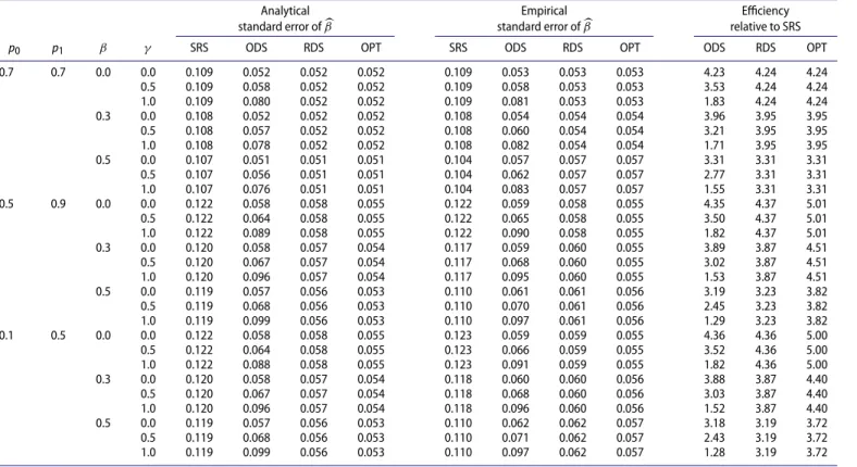
Table 1.Simulation results for linear regression with discrete covariates.
Analytical Empirical Efficiency
standard error ofβ standard error ofβ relative to SRS
p0 p1 β γ SRS ODS RDS OPT SRS ODS RDS OPT ODS RDS OPT
0.7 0.7 0.0 0.0 0.109 0.052 0.052 0.052 0.109 0.053 0.053 0.053 4.23 4.24 4.24
0.5 0.109 0.058 0.052 0.052 0.109 0.058 0.053 0.053 3.53 4.24 4.24
1.0 0.109 0.080 0.052 0.052 0.109 0.081 0.053 0.053 1.83 4.24 4.24
0.3 0.0 0.108 0.052 0.052 0.052 0.108 0.054 0.054 0.054 3.96 3.95 3.95
0.5 0.108 0.057 0.052 0.052 0.108 0.060 0.054 0.054 3.21 3.95 3.95
1.0 0.108 0.078 0.052 0.052 0.108 0.082 0.054 0.054 1.71 3.95 3.95
0.5 0.0 0.107 0.051 0.051 0.051 0.104 0.057 0.057 0.057 3.31 3.31 3.31
0.5 0.107 0.056 0.051 0.051 0.104 0.062 0.057 0.057 2.77 3.31 3.31
1.0 0.107 0.076 0.051 0.051 0.104 0.083 0.057 0.057 1.55 3.31 3.31
0.5 0.9 0.0 0.0 0.122 0.058 0.058 0.055 0.122 0.059 0.058 0.055 4.35 4.37 5.01
0.5 0.122 0.064 0.058 0.055 0.122 0.065 0.058 0.055 3.50 4.37 5.01
1.0 0.122 0.089 0.058 0.055 0.122 0.090 0.058 0.055 1.82 4.37 5.01
0.3 0.0 0.120 0.058 0.057 0.054 0.117 0.059 0.060 0.055 3.89 3.87 4.51
0.5 0.120 0.067 0.057 0.054 0.117 0.068 0.060 0.055 3.02 3.87 4.51
1.0 0.120 0.096 0.057 0.054 0.117 0.095 0.060 0.055 1.53 3.87 4.51
0.5 0.0 0.119 0.057 0.056 0.053 0.110 0.061 0.061 0.056 3.19 3.23 3.82
0.5 0.119 0.068 0.056 0.053 0.110 0.070 0.061 0.056 2.45 3.23 3.82
1.0 0.119 0.099 0.056 0.053 0.110 0.097 0.061 0.056 1.29 3.23 3.82
0.1 0.5 0.0 0.0 0.122 0.058 0.058 0.055 0.123 0.059 0.059 0.055 4.36 4.36 5.00
0.5 0.122 0.064 0.058 0.055 0.123 0.066 0.059 0.055 3.52 4.36 5.00
1.0 0.122 0.088 0.058 0.055 0.123 0.091 0.059 0.055 1.82 4.36 5.00
0.3 0.0 0.120 0.058 0.057 0.054 0.118 0.060 0.060 0.056 3.88 3.87 4.40
0.5 0.120 0.067 0.057 0.054 0.118 0.068 0.060 0.056 3.03 3.87 4.40
1.0 0.120 0.096 0.057 0.054 0.118 0.096 0.060 0.056 1.52 3.87 4.40
0.5 0.0 0.119 0.057 0.056 0.053 0.110 0.062 0.062 0.057 3.18 3.19 3.72
0.5 0.119 0.068 0.056 0.053 0.110 0.071 0.062 0.057 2.43 3.19 3.72
1.0 0.119 0.099 0.056 0.053 0.110 0.097 0.062 0.057 1.28 3.19 3.72
NOTE: SRS, ODS, RDS, and OPT denote simple random sampling, outcome-dependent sampling, residual-dependent sampling, and optimal design, respectively. Each entry is based on 10,000 replicates.
For linear regression,Corollary 1shows that the optimal design does not need to stratify on Z. Then treating var(X|Z) as a constant reduces the optimal design to residual-dependent sam-pling, which is always more efficient than outcome-dependent sampling whether var(X|Z)is a constant or not. For logistic regression, treating var(X|Z)as a constant reduces the optimal design to stratified case-control sampling. In this situation, we do not know the optimal stratum sizes because var(Dμ|R = 1,Z) =1/4 for anyZ(provided thatτ < 2E(Y)). If var(X|Z) is a constant, then the stratum sizes are irrelevant to design efficiency. If the spread of var(X|Z) is large, then stratified case-control sampling with equal stratum sizes can be more or less efficient than case-control sampling when the strata with larger values of var(X|Z)are less or more prevalent than the other strata, respectively. For more complex models, such as the proportional hazards model, treating var(X|Z)as a constant is appropriate when the spread of var(X|Z)is small or when var(X|Z)and var(Dμ|R=1,Z)are positively correlated. Treat-ing var(X|Z)as a constant can reduce design efficiency when the spread of var(X|Z)is large and var(X|Z)and var(Dμ|R=1,Z) are negatively correlated.
3. Simulation Studies
We conducted extensive simulation studies to compare the effi-ciencies of various two-phase designs in realistic settings. In the first set of studies, we considered a continuous outcome with discrete covariates. Specifically, we setZandX|Zto Bern(0.5) and Bern{I(Z = 0)p0 +I(Z = 1)p1}, respectively, with 0 < p0 < 1 and 0 < p1 < 1. We generated the outcome from the
linear modelY =βX+γZ+1, where1is a standard normal random variable independent ofXandZ. We setn=4000 and considered four sampling strategies at the second phase: sim-ple random sampling selects 400 subjects randomly; outcome-dependent sampling selects 200 subjects with the highest and 200 subjects with the lowest values of Y; residual-dependent sampling selects 200 subjects with the highest and 200 subjects with the lowest values ofY−μ(Z), whereμ(Z) = α+γZ, andα and γ are the least-squares estimates from the linear regression ofYonZ; and optimal sampling selects 200 subjects with the highest and 200 subjects with the lowest values of {Y−μ(Z)} {var(X|Z)}1/2, where var(X|Z = j) = pj(1−pj)
(j=0, 1). We performed maximum likelihood estimation (Tao, Zeng, and Lin2017) under the four designs. We evaluated the efficiency of each design according to the empirical variance of
β. In addition, we compared the analytical varianceVβgiven in
Theorem 1with the empirical variance.
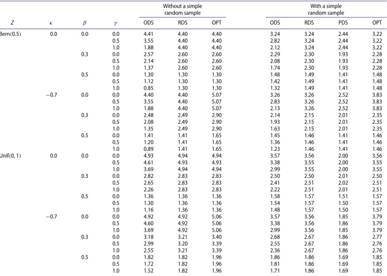
Table 2. Relative efficiencies of two-phase designs to simple random sampling for linear regression with a continuous expensive covariate.
Without a simple With a simple
random sample random sample
Z κ β γ ODS RDS OPT ODS RDS PDS OPT
Bern(0.5) 0.0 0.0 0.0 4.41 4.40 4.40 3.24 3.24 2.44 3.22
0.5 3.55 4.40 4.40 2.82 3.24 2.44 3.22
1.0 1.88 4.40 4.40 2.12 3.24 2.44 3.22
0.3 0.0 2.57 2.60 2.60 2.29 2.30 1.93 2.28
0.5 2.14 2.60 2.60 2.08 2.30 1.93 2.28
1.0 1.37 2.60 2.60 1.74 2.30 1.93 2.28
0.5 0.0 1.30 1.30 1.30 1.48 1.49 1.41 1.48
0.5 1.12 1.30 1.30 1.42 1.49 1.41 1.48
1.0 0.85 1.30 1.30 1.32 1.49 1.41 1.48
−0.7 0.0 0.0 4.40 4.40 5.07 3.26 3.26 2.52 3.83
0.5 3.55 4.40 5.07 2.83 3.26 2.52 3.83
1.0 1.88 4.40 5.07 2.13 3.26 2.52 3.83
0.3 0.0 2.48 2.49 2.90 2.14 2.15 2.01 2.35
0.5 2.08 2.49 2.90 1.93 2.15 2.01 2.35
1.0 1.35 2.49 2.90 1.63 2.15 2.01 2.35
0.5 0.0 1.41 1.41 1.65 1.45 1.46 1.41 1.46
0.5 1.20 1.41 1.65 1.36 1.46 1.41 1.46
1.0 0.89 1.41 1.65 1.23 1.46 1.41 1.46
Unif(0, 1) 0.0 0.0 0.0 4.93 4.94 4.94 3.57 3.56 2.00 3.56
0.5 4.61 4.93 4.93 3.38 3.55 2.00 3.55
1.0 3.69 4.94 4.94 2.99 3.55 2.00 3.55
0.3 0.0 2.82 2.83 2.83 2.50 2.50 2.01 2.50
0.5 2.65 2.83 2.83 2.41 2.51 2.02 2.51
1.0 2.26 2.83 2.83 2.22 2.51 2.01 2.51
0.5 0.0 1.36 1.36 1.36 1.58 1.57 1.51 1.57
0.5 1.30 1.36 1.36 1.54 1.57 1.50 1.57
1.0 1.16 1.36 1.36 1.48 1.57 1.50 1.57
−0.7 0.0 0.0 4.92 4.92 5.06 3.57 3.56 1.85 3.79
0.5 4.60 4.92 5.06 3.38 3.56 1.86 3.79
1.0 3.69 4.92 5.06 2.99 3.56 1.85 3.79
0.3 0.0 3.18 3.21 3.40 2.68 2.67 1.86 2.77
0.5 2.99 3.20 3.39 2.55 2.67 1.86 2.76
1.0 2.55 3.21 3.39 2.36 2.67 1.86 2.76
0.5 0.0 1.82 1.82 1.96 1.86 1.86 1.69 1.85
0.5 1.72 1.82 1.96 1.81 1.86 1.69 1.85
1.0 1.52 1.82 1.96 1.71 1.86 1.69 1.85
NOTE: ODS, RDS, PDS, and OPT denote outcome-dependent sampling, residual-dependent sampling, probability-dependent sampling, and optimal design, respectively. Each entry is based on 10,000 replicates.
be small (relative to the true value) and in the same direction for different designs, such that the ordering of the design efficiencies is unaltered.
In the second set of simulation studies, we considered a continuous instead of a discrete expensive covariate. Specif-ically, we set X = 0.2Z + (1 + κZ)1/22, where 2 is a standard normal random variable independent of Z and 1, andκ is a parameter that controls the value of var(X|Z). We setZto Bern(0.5)or Unif(0, 1). In addition to the two-phase designs considered in the first set of studies, we included four designs that select a simple random sample of 200 subjects at the beginning of the second phase. The following strategies were adopted to select the remaining 200 subjects in the sec-ond phase: outcome-dependent sampling selects subjects with extreme values ofY; residual-dependent sampling selects sub-jects with extreme values ofY−μ(Z); probability-dependent sampling (Zhou et al.2014) selects subjects with extreme values of X, where X is the predicted value of X from the linear regression ofX on Y stratified by Z when Z is discrete and from the linear regression ofXon(Y,Z)whenZis continuous; and optimal sampling selects subjects with extreme values of {Y−μ(Z)} {var(X|Z)}1/2, where var(X|Z)is estimated from the simple random sample.
The results for the second set of studies are summarized in Table 2 and Supplementary Tables S2 and S3. In general, the designs that do not require a simple random sample at the beginning of the second phase are more efficient than those that do. Among designs that contain a simple random sample, the design that adopts the optimal sampling ruleRoptlinearto select the remaining subjects in the second phase is the most efficient.
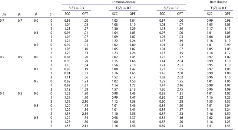
Table 3.Relative efficiencies of other two-phase designs to case-control sampling for logistic regression.
Common disease Rare disease
E(Z)=0.3 E(Z)=0.5 E(Z)=0.7 E(Z)=0.1
p0 p1 β γ SCC OPT SCC OPT SCC OPT SCC OPT
0.7 0.7 0.0 0 0.98 1.00 1.03 1.04 0.97 1.00 0.99 0.98
1 1.04 1.05 1.08 1.10 1.03 1.07 1.05 1.05
2 1.23 1.27 1.30 1.29 1.18 1.19 1.17 1.17
0.3 0 0.96 1.01 1.04 1.05 0.97 1.00 1.01 1.03
1 1.04 1.07 1.09 1.07 1.05 1.03 1.06 1.05
2 1.24 1.28 1.22 1.26 1.17 1.19 1.18 1.19
0.5 0 0.99 1.01 1.02 1.00 1.01 1.04 1.01 0.99
1 1.08 1.10 1.05 1.07 1.04 1.07 1.05 1.03
2 1.28 1.33 1.23 1.26 1.13 1.15 1.14 1.12
0.5 0.9 0.0 0 0.84 1.20 1.02 1.45 1.25 1.77 0.97 1.02
1 0.90 1.29 1.15 1.66 1.44 2.04 0.99 1.10
2 1.10 1.64 1.56 2.18 1.71 2.51 0.95 1.10
0.3 0 0.83 1.19 1.00 1.47 1.27 1.85 0.97 1.05
1 0.91 1.31 1.16 1.65 1.45 2.08 0.99 1.08
2 1.11 1.56 1.52 2.17 1.82 2.62 0.96 1.10
0.5 0 0.82 1.23 1.02 1.50 1.29 1.95 1.01 1.06
1 0.92 1.31 1.14 1.72 1.47 2.16 0.98 1.07
2 1.12 1.58 1.57 2.18 1.86 2.75 0.96 1.09
0.1 0.5 0.0 0 1.22 1.80 0.98 1.46 0.85 1.21 1.01 1.02
1 1.29 1.90 0.99 1.47 0.86 1.22 1.16 1.22
2 1.52 2.10 1.12 1.58 0.90 1.28 1.55 1.56
0.3 0 1.20 1.73 1.01 1.46 0.84 1.20 1.01 1.04
1 1.29 1.84 1.01 1.41 0.84 1.17 1.16 1.24
2 1.58 2.19 1.10 1.58 0.87 1.23 1.46 1.50
0.5 0 1.22 1.74 0.98 1.37 0.84 1.16 1.02 1.06
1 1.27 1.80 1.00 1.41 0.87 1.20 1.16 1.23
2 1.53 2.11 1.16 1.58 0.89 1.23 1.41 1.43
NOTE: SCC and OPT denote stratified case-control sampling and optimal design, respectively. Each entry is based on 10,000 replicates.
case-control sampling, both of which select all cases and an equal number of controls in the second phase.
The results for the third set of studies are summarized in Table 3and Supplementary Tables S4 and S5. When var(X|Z) is a constant and γ = 0, all designs are equally efficient. Whenγ = 0, stratified case-control sampling and optimal design are more efficient than case-control sampling, and the efficiency gain increases asγincreases. In addition, the similar efficiencies between stratified case-control sampling and opti-mal design confirm that the stratum size is irrelevant to the design efficiency. When var(X|Z)is a nontrivial function ofZ, the optimal design is substantially more efficient than the other two designs. Stratified case-control sampling can be less efficient than case-control sampling when var(X|Z)is larger in the more prevalent stratum. These results disprove the common belief that it is always desirable to pursue an equal number of subjects per stratum.
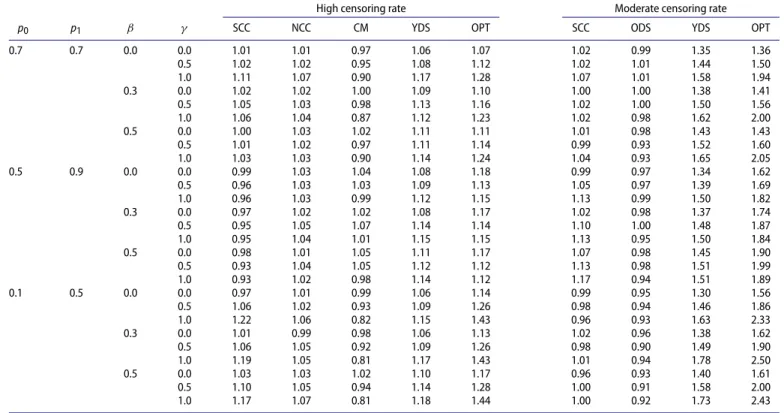
In the last set of simulation studies, we considered a poten-tially censored event time. We generatedXandZin the same manner as in the first set of studies. We generatedT from the Weibull proportional hazards model with cumulative hazard function 0.1t0.7exp(βX+γZ). In addition, we generated the censoring time C from a Uniform(0,c1) distribution, where c1 = 1 or 5, yielding 85%–94% or 64%–84% censoring, to be referred to as high and moderate censoring rates, respectively. We set the cohort size n = 2000. In the case of moderate censoring rate, we setn2 = 400 and compared the optimal design with four sampling strategies that select a subset of cases: case-cohort sampling (Cai and Zeng2007) selects 200 cases and 200 controls; stratified case-cohort sampling (Borgan et al.2000) selects 100 cases and 100 controls from each of the
two strata; general failure-time outcome-dependent sampling (Ding et al. 2014) selects 100 cases with the largest and 100 cases with the smallest observed event times in addition to a subcohort of 200 subjects; andY-dependent sampling (Lawless 2018) selects the 200 smallest observed event times and the 200 largest censored observations. In the case of high censoring rate, we compared the optimal design with four sampling strategies that select all cases and an equal number of controls in the second phase: case-cohort sampling (Prentice1986); stratified case-cohort sampling; nested case-control sampling (Thomas 1977) with one control for each observed event time; counter-matching (Langholz and Borgan1995), which selects one con-trol withZ = 0 for each case withZ = 1 and vice versa; and Y-dependent sampling.
The results for the last set of studies are summarized in Table 4 and Supplementary Tables S6 and S7. The optimal design is much more efficient than the other designs in most situations. TheY-dependent sampling design is as efficient as the optimal design when var(X|Z)is a constant andγ =0. In this situation,Dμ=− (T), which is a monotone function of T. Therefore, selecting the smallest observed event times and the largest censored observations is equivalent to selecting subjects with the largest and smallest values ofDμ, respectively.
4. Applications
4.1. National Heart, Lung, and Blood Institute Exome Sequencing Project
Table 4. Relative efficiencies of other two-phase designs to case-cohort sampling under the proportional hazards model.
High censoring rate Moderate censoring rate
p0 p1 β γ SCC NCC CM YDS OPT SCC ODS YDS OPT
0.7 0.7 0.0 0.0 1.01 1.01 0.97 1.06 1.07 1.02 0.99 1.35 1.36
0.5 1.02 1.02 0.95 1.08 1.12 1.02 1.01 1.44 1.50
1.0 1.11 1.07 0.90 1.17 1.28 1.07 1.01 1.58 1.94
0.3 0.0 1.02 1.02 1.00 1.09 1.10 1.00 1.00 1.38 1.41
0.5 1.05 1.03 0.98 1.13 1.16 1.02 1.00 1.50 1.56
1.0 1.06 1.04 0.87 1.12 1.23 1.02 0.98 1.62 2.00
0.5 0.0 1.00 1.03 1.02 1.11 1.11 1.01 0.98 1.43 1.43
0.5 1.01 1.02 0.97 1.11 1.14 0.99 0.93 1.52 1.60
1.0 1.03 1.03 0.90 1.14 1.24 1.04 0.93 1.65 2.05
0.5 0.9 0.0 0.0 0.99 1.03 1.04 1.08 1.18 0.99 0.97 1.34 1.62
0.5 0.96 1.03 1.03 1.09 1.13 1.05 0.97 1.39 1.69
1.0 0.96 1.03 0.99 1.12 1.15 1.13 0.99 1.50 1.82
0.3 0.0 0.97 1.02 1.02 1.08 1.17 1.02 0.98 1.37 1.74
0.5 0.95 1.05 1.07 1.14 1.14 1.10 1.00 1.48 1.87
1.0 0.95 1.04 1.01 1.15 1.15 1.13 0.95 1.50 1.84
0.5 0.0 0.98 1.01 1.05 1.11 1.17 1.07 0.98 1.45 1.90
0.5 0.93 1.04 1.05 1.12 1.12 1.13 0.98 1.51 1.99
1.0 0.93 1.02 0.98 1.14 1.12 1.17 0.94 1.51 1.89
0.1 0.5 0.0 0.0 0.97 1.01 0.99 1.06 1.14 0.99 0.95 1.30 1.56
0.5 1.06 1.02 0.93 1.09 1.26 0.98 0.94 1.46 1.86
1.0 1.22 1.06 0.82 1.15 1.43 0.96 0.93 1.63 2.33
0.3 0.0 1.01 0.99 0.98 1.06 1.13 1.02 0.96 1.38 1.62
0.5 1.06 1.05 0.92 1.09 1.26 0.98 0.90 1.49 1.90
1.0 1.19 1.05 0.81 1.17 1.43 1.01 0.94 1.78 2.50
0.5 0.0 1.03 1.03 1.02 1.10 1.17 0.96 0.93 1.40 1.61
0.5 1.10 1.05 0.94 1.14 1.28 1.00 0.91 1.58 2.00
1.0 1.17 1.07 0.81 1.18 1.44 1.00 0.92 1.73 2.43
NOTE: SCC, NCC, CM, ODS, YDS, and OPT denote stratified case-cohort sampling, nested case-control sampling, counter-matching, general failure-time outcome-dependent sampling,Y-dependent sampling, and optimal design, respectively. Each entry is based on 10,000 replicates.
protein-coding regions of the human genome that are associated with heart, lung, and blood disorders. The project performed whole-exome sequencing on 4494 subjects from seven large cohorts and consisted of several studies, each focusing on a particular outcome (Lin, Zeng, and Tang2013). The majority of the studies adopted two-phase designs. For example, the study on body mass index selected 659 subjects with body mass index less than 25 kg/m2 or greater than 40 kg/m2. The study on blood pressure selected 806 subjects from the upper and lower 0.2%–1.0% of the blood pressure distribution adjusted for age, gender, race, body mass index, and anti-hypertensive medication. The study on low-density lipoprotein cholesterol selected 657 subjects with extremely high or low values of low-density lipoprotein cholesterol adjusted for age, gender, race, and lipid medication. In addition to the two-phase studies, the project obtained a simple random sample of 964 subjects with measurements on a common set of phenotypes, referred to as the “deeply phenotyped reference.” We used this deeply phenotyped reference to evaluate the efficiencies of two-phase designs.
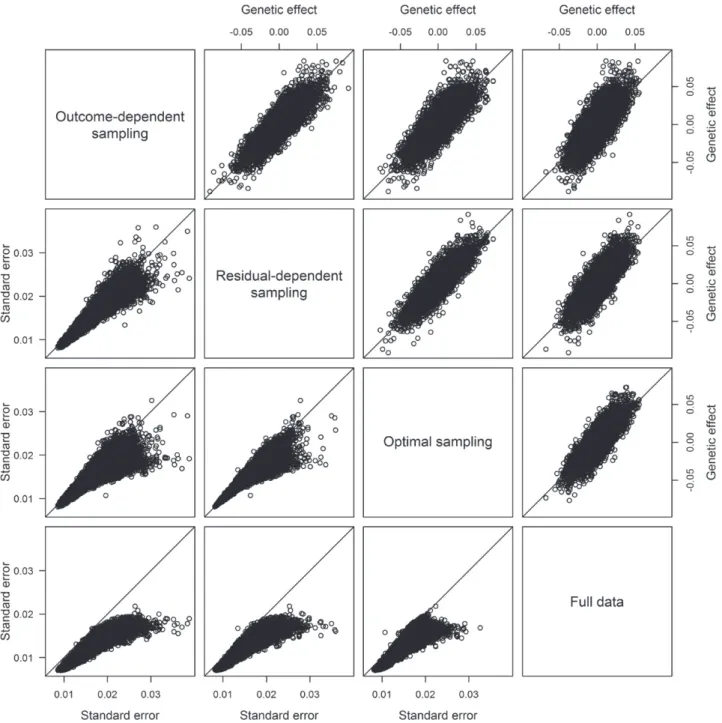
We considered log-transformed body mass index as the out-come of interest and included age, gender, race, and cohort indi-cators as inexpensive covariates. We restricted our analysis to the 43,245 single-nucleotide polymorphisms (SNPs) with minor allele frequencies greater than 5%. We chose the additive genetic model, under which the genetic variable codes the number of minor alleles that a subject carries at a variant site. We set n2 = 300 and considered three sampling strategies: outcome-dependent sampling; residual-outcome-dependent sampling; and optimal sampling. The probability-dependent sampling design (Zhou et al.2014) is not applicable because it does not allow discrete expensive covariates. Because age, gender, and cohort indicators
are independent of SNPs, we only need to estimate the condi-tional variance of the genetic variable given race when imple-menting the optimal design. Because this conditional variance depends on the genetic variable, the optimal sampling rule is specific to each SNP.
Figure 1compares the estimates of the genetic effects and the standard error estimates among the three two-phase designs and the full-data analysis. The effect estimates are similar among the three two-phase designs and are close to those of the full-data analysis. The standard error estimates under the optimal design tend to be smaller than those under residual-dependent sampling, which tend to be smaller than those under outcome-dependent sampling. These results show that residual-dependent sampling can yield more precise genetic effect esti-mates and higher power than outcome-dependent sampling for genome-wide association studies, and the optimal design can be more efficient than residual-dependent sampling for candidate-gene studies.
4.2. National Wilms’ Tumor Study
The National Wilms’ Tumor Study Group conducted a series of studies on Wilms’ tumor, which is a rare childhood kidney cancer. We used data on 4028 patients from the group’s third and fourth clinical trials (D’angio et al.1989; Green et al.1998) to evaluate the effects of tumor histological type, stage, and age at diagnosis on disease relapse. The censoring rate was approximately 86%. This dataset was analyzed previously by Breslow and Chatterjee (1999).
Figure 1. Estimates of the genetic effects, shown in the upper right triangle, and standard errors, shown in the lower left triangle, from the linear regression of the log-transformed body mass index on SNPs in the deeply phenotyped reference for the National Heart, Lung, and Blood Institute Exome Sequencing Project.
expensive and time-consuming. If a two-phase design had been adopted to assess histological type at the central facility for only a small subset of patients, then the cost of the trials would have been drastically reduced. In fact, several follow-up studies by the National Wilms’ Tumor Study Group adopted the nested case-control design (Green et al.2001; Warwick et al.2010).
We defined two strata according to unfavorable versus favor-able local histological assessment. We considered two scenarios with different values ofn2. In the first scenario, we setn2=400 and considered five sampling strategies: case-cohort sampling; stratified case-cohort sampling; general failure-time outcome-dependent sampling;Y-dependent sampling; and optimal sam-pling. To ensure model identifiability and numerical stability, we required the second-phase sample size for each stratum to
Table 5. Estimates of log hazard ratios, with standard error estimates in parentheses, from the proportional hazards regression analysis of the National Wilms’Tumor Study.
Histological assessment Tumor stage
n2 Design Central Local II III IV Age
400 CC 1.573 (0.359) 0.114 (0.291) 0.682 (0.125) 0.793 (0.125) 1.067 (0.141) 0.078 (0.015)
SCC 1.579 (0.322) 0.068 (0.297) 0.677 (0.127) 0.790 (0.127) 1.092 (0.143) 0.078 (0.015)
ODS 1.882 (0.382) −0.127 (0.302) 0.692 (0.127) 0.795 (0.128) 1.083 (0.145) 0.080 (0.015) YDS 2.210 (0.269) −0.034 (0.229) 0.704 (0.129) 0.835 (0.130) 1.113 (0.147) 0.080 (0.015)
OPT 1.549 (0.260) 0.161 (0.258) 0.666 (0.124) 0.781 (0.123) 1.151 (0.139) 0.077 (0.015)
1142 CC 1.513 (0.219) 0.128 (0.199) 0.676 (0.131) 0.789 (0.131) 1.062 (0.146) 0.077 (0.015)
SCC 1.578 (0.193) 0.083 (0.195) 0.665 (0.113) 0.788 (0.112) 1.134 (0.132) 0.077 (0.015)
NCC 1.510 (0.226) 0.133 (0.198) 0.675 (0.132) 0.789 (0.132) 1.063 (0.147) 0.077 (0.015)
CM 1.585 (0.192) 0.077 (0.200) 0.666 (0.117) 0.789 (0.117) 1.134 (0.159) 0.077 (0.016)
YDS 1.947 (0.202) −0.109 (0.184) 0.699 (0.124) 0.838 (0.124) 1.110 (0.140) 0.072 (0.015)
OPT 1.424 (0.185) 0.228 (0.181) 0.667 (0.111) 0.777 (0.111) 1.135 (0.141) 0.075 (0.015)
4028 FC 1.444 (0.135) 0.203 (0.144) 0.662 (0.122) 0.802 (0.121) 1.137 (0.135) 0.071 (0.015)
NOTE: CC, SCC, ODS, YDS, OPT, NCC, CM, and FC denote case-cohort sampling, stratified case-cohort sampling, general failure-time outcome-dependent sampling,Y -dependent sampling, optimal design, nested case-control sampling, counter-matching, and full-cohort, respectively. Estimates of log hazard ratios and standard errors under the CC, SCC, ODS, NCC, and CM designs are averaged over 1000 replicates.
Table 5 shows the estimation results for the proportional hazards model under the two-phase designs and the full-cohort analysis. The log hazard-ratio estimates under most two-phase designs are close to their full-cohort counterparts. The effect of local histological assessment is not significant after adjusting for central histological assessment. The standard error estimate of central histological assessment under the optimal design is smaller than that under the other two-phase designs. These results are consistent with our theoretical and simulation results.
5. Discussion
As mentioned inSection 1, the existing literature on two-phase studies is concerned primarily with the inference procedures rather than the design aspects. In particular, Tao, Zeng, and Lin (2017) studied efficient inference under two-phase sampling but did not consider design efficiency at all. To investigate design efficiency, one has to know exactly how the design parameter affects the efficiency bound. To this end,Theorem 1provides for the first time an explicit form for the efficiency bound. It reveals an important fact that the efficiency depends on the conditional variance of the expensive covariate given inexpensive covariates. Theorem 2, together with Corollaries 1 and 2, provides the optimal sampling rules for two-phase studies. No such result exists in the literature, despite extensive prior research on two-phase studies. Indeed, our work shows that the commonly used two-phase designs are not optimal. The proofs ofTheorems 1 and 2and Corollaries 1and 2 require considerable technical innovation.
As shown inSection 2.4, the optimal design for linear regres-sion does not need to stratify onZ. The optimal designs for logistic regression and proportional hazards regression do not need to stratify onZwhenγ = 0and var(X|Z)is a constant. In other situations, we need to divideZinto a few strata when implementing the “optimal” design. DiscretizingZis a common practice to facilitate implementation of two-phase studies. The resulting design should converge to the optimal one as the number of strata increases.
The efficiency bound under the condition ofβ =o(1)is of practical importance because design efficiency matters the most whenβ is small, and it provides a good approximation to the efficiency bound for largeβ, as confirmed by our numerical
studies. In the simulation studies, we considered β as large as 0.5, which corresponds to 50% of the error variance, odds ratio of 1.65, and hazard ratio of 1.65 under the linear, logistic, and proportional hazards models, respectively. For the National Heart, Lung, and Blood Institute Exome Sequencing Project, the estimates of the genetic effects on standardized log-transformed body mass index range from−0.39 to 0.32. For genetic studies with binary traits, the odds ratio estimates are rarely larger than 1.3 (Schizophrenia Working Group of the Psychiatric Genomics Consortium2014; Xue et al.2018). Thus, the values ofβis our simulation studies cover the typical values in genetic studies, for which two-phase designs are most commonly adopted. For the National Wilms’ Tumor Study, the hazard ratio for central histology is 4.24. In all these situations, the proposed designs are more efficient than the existing designs.
Our theory does not require every study subject to have a positive probability of being selected in the second phase and thus can accommodate the outcome-dependent sampling and residual-dependent sampling described in Lin, Zeng, and Tang (2013), theY-dependent sampling proposed by Lawless (2018), and the optimal design. Naturally, we can estimate only the parameters that are informed by the observed data. For example, if we sample only from the extreme tails of the outcome distribution, then we cannot nonparametrically identify the dis-tribution in the middle, although we can estimate the regression parameters. The existing semiparametric efficiency theory with missing data (Robins, Hsieh, and Newey1995) requires positive selection probability for every study subject, so as to identify all parameters.
We evaluated the efficiencies of existing two-phase designs and developed optimal designs. A closely related problem is to calculate the power and sample size for a specific design. The variance formula given in (2) can be used for power and sample size calculations under any two-phase design, provided that the first-phase data and the first and second moments of the conditional distribution ofXgivenZare available.
We assumed that X is a scalar. For multivariate X, var(Dμ|R = 1,Z)is still a scalar, whereas var(X|Z)becomes a matrix. We can still useTheorem 1 to calculateVβ for any two-phase design. The added complexity lies in the estimation of var(X|Z). We can define the design efficiency based on the trace or determinant of Vβ, with the corresponding optimal designs being “A-optimal” or “D-optimal,” respectively. Opti-mality criteria have been discussed in the design of experi-ments literature; see Fedorov and Leonov (2013). The use of different optimality criteria, such as the determinant, trace, or eigenvalues of the covariance matrix, can yield different optimal designs, and which should be chosen in practice depends on the scientific question of interest. Because var(Dμ|R = 1,Z)is a scalar, the optimal designs still select subjects with the largest or smallest values ofDμin each stratum ofZand favors the strata with the largest values of the trace or determinant of var(X|Z). Theorem 2andCorollaries 1and2with multivariateXcan be derived similarly to the case of a scalarX.
Some of the early research on two-phase designs was con-cerned with the main effects of Z, with X as an expensive confounder, and the inference procedures were typically based only on the second-phase data (White1982; Breslow and Cain 1988). Because our efficient inference procedures utilize the data onZfor all study subjects, our estimator ofγ under any two-phase design is essentially as efficient as the maximum likelihood estimator based on the full data.
We dealt with a single outcome. In large-scale cohort studies and electronic heath record systems, a number of potentially correlated outcomes are observed. An interesting topic of inves-tigation is the optimal two-phase design when multiple contin-uous outcomes are of equal importance. Tao et al. (2015) con-sidered two multivariate outcome-dependent sampling designs: the first design selects an equal number of subjects from the upper and lower tails of each outcome distribution; the second design selects subjects from one tail of each outcome distribu-tion and uses a random sample as a common comparison group. Although their simulation results indicated that the first design is more efficient than the second one, it is unclear whether or not this conclusion holds broadly. Another interesting topic is the optimal design when the outcome is longitudinal repeated mea-sures (Schildcrout, Garbett, and Heagerty 2013). Our frame-work can be used to derive optimal designs for studies with multiple or longitudinal outcomes.
Appendix: Technical Details
LetSη(h1)denote the score forηalong the submodel→η(h1)for
one complete observation(Y,X,Z), whereh1is the tangent direction
along this submodel in thatdη(h1)/d|=0 = h1, andη0(h1) = η.
LetUθdenote the score forθ,Uη(h1)denote the score forηalong the
submodelη(h1), andUf(h2)denote the score forfalong the submodel
{1+h2(x,z)}f(x,z)under the two-phase design, whereh2belongs to
L02(f)=h:hfdxdz=0,h2fdxdz<∞. Clearly,
Uθ=RDμ(1,X,ZT)T+(1−R)E
Dμ(1,X,ZT)TY,Z
,
Uη(h1)=RSη(h1)+(1−R)ESη(h1)Y,Z,
Uf(h2)=Rh2(X,Z)+(1−R)E{h2(X,Z)|Y,Z}.
The information operator is
⎛ ⎜ ⎝
Uθ∗Uθ Uθ∗Uη Uθ∗Uf Uη∗Uθ Uη∗Uη Uη∗Uf Uf∗Uθ Uf∗Uη Uf∗Uf
⎞ ⎟ ⎠,
whereUθ∗,Uη∗, andUf∗are the adjoint operators ofUθ,Uη, andUf, respectively. Whenβ=0,DμandSη(h1)do not depend onX, and the
calculations of the information operators can be simplified greatly. We utilize this property to derive the semiparametric efficiency bound of estimatingβunder general two-phase designs.
Letθ0,η0, andf0be the true values ofθ,η, andf, respectively. We
impose the following regularity conditions:
Condition A.1. The set of covariates(X,Z)has bounded support.
Condition A.2. If there exist two sets of parameters(θ1,η1,f1)and
(θ2,η2,f2)such that
pθ1,η1(Y|X,Z)f1(X,Z)=pθ2,η2(Y|X,Z)f2(X,Z),
where(Y,X,Z)lies inC = {(y,x,z): Pr(R= 1|y,z) >0}, thenθ1 = θ2,η1=η2, andf1=f2. In addition, if there exists a constant vectorv
such that
[∂log{pθ0,η0(y1|x,z)/pθ0,η0(y2|x,z)}/∂θ]
Tv=0
for any(yi,x,z)∈C(i=1, 2), thenv=0.
Condition A.3. The density functionf0is positive in its support and
q-times continuously differentiable with respect to a suitable measure, whereq>dz/2, anddzis the dimension ofZ.
Condition A.4. The function E(R|Y,Z)isq-times continuously differ-entiable with respect toZin its support.
Remark A.1. Conditions A.2–A.4correspond to Conditions (C.1)– (C.4) in Tao, Zeng, and Lin (2017); see Remark S.1 in Tao, Zeng, and Lin (2017) for discussion of these conditions.
Becauseα,β, andγ can be perturbed independently, we can write U∗θUθas
⎛ ⎝U
∗
αUα Uα∗Uβ Uα∗Uγ
Uβ∗Uα Uβ∗Uβ Uβ∗Uγ Uγ∗Uα Uγ∗Uβ Uγ∗Uγ
⎞ ⎠,
whereUα,Uβ, andUγ denote the scores forα,β, andγ, respectively, andUα∗,Uβ∗, andU∗γdenote the adjoint operators ofUα,Uβ, andUγ, respectively. We state and prove the following two lemmas, which will be used in the proof ofTheorem 1.
Lemma A.1. Whenβ=0, the information operators for(θ,η,f)are
Uα∗Uα =E
D2μ ,Uγ∗Uγ =E
D2μZZT , Uα∗Uγ =E
D2μZT ,
Uα∗Uβ =E
D2μE(X|Z)
,Uβ∗Uγ =E
D2μE(X|Z)ZT
,
Uβ∗Uβ =E
D2μE(X|Z)2
+E
RD2μvar(X|Z)
,
U∗αUη(h1)=EDμSη(h1), Uγ∗Uη(h1)=EDμZSη(h1),
Uβ∗Uη(h1)=EDμE(X|Z)Sη(h1), Uη∗Uη(h1)=S∗ηSη(h1),
Uα∗Uf(h2)=0,Uγ∗Uf(h2)=0,Uη∗Uf(h2)=0,
U∗βUf(h2)=EERDμ|Z{X−E(X|Z)}h2(X,Z),
Uf∗Uf(h2)=E(R|Z)h2(X,Z)+E(1−R|Z)E{h2(X,Z)|Z},
Proof of Lemma A.1. The calculations of the information operators follow from the derivations in the proof of Theorem S.2 in Tao, Zeng, and Lin (2017) and the fact thatYandRare independent ofX condi-tional onZwhenβ=0.
Lemma A.2. LetM2 = Uf(Uf∗Uf)−1Uf∗be the projection operator
onto the score space off. Suppose thath3 belongs toL02(P), where
Pis the probability measure indexed by(θ,η,f). Whenβ = 0 and
Conditions A.2–A.4hold,
M2h3=RE(R|Z)−1{E(Rh3|X,Z)−E(Rh3|Z)} +E(h3|Z), (A.1)
where we define E(R|Z)−1=0 whenever E(R|Z)=0.
Proof of Lemma A.2. We first derive Uf∗(h3). By the definition of
adjoint operators,
Uf(h2),h3 = h2,Uf∗(h3), (A.2)
where·,·denotes the inner product in Hilbert space. Underβ =
0,Y andRare independent ofXgivenZ, such that the left side of Equation (A.2) equals
E([Rh2(X,Z)+(1−R)E{h2(X,Z)|Z}]h3(Y,X,Z))
=E [E{Rh3(Y,X,Z)|X,Z}h2(X,Z)]
+E(E [E{(1−R)h3(Y,X,Z)|Z}h2(X,Z)|Z])
=E([E{Rh3(Y,X,Z)|X,Z} +E{(1−R)h3(Y,X,Z)|Z}]h2(X,Z)).
Thus,
U∗f(h3)=E{Rh3(Y,X,Z)|X,Z} +E{(1−R)h3(Y,X,Z)|Z}. (A.3)
Next, we calculate(Uf∗Uf)−1(h2). Assume, without loss of generality,
that(U∗fUf)−1(h2)=A(X,Z)h2(X,Z)+B(X,Z)E{h2(X,Z)|Z}, where
A(X,Z)andB(X,Z)belong toL2(f)=h:h2fdxdz<∞. Clearly,
h2(X,Z)=(Uf∗Uf)−1(Uf∗Uf)(h2)
=A(X,Z)[E(R|Z)h2(X,Z)+ {1−E(R|Z)}E{h2(X,Z)|Z}]
+B(X,Z)EE(R|Z)h2(X,Z)
+ {1−E(R|Z)}E{h2(X,Z)|Z} |Z
=A(X,Z)E(R|Z)h2(X,Z)
+ {A(X,Z)−A(X,Z)E(R|Z)+B(X,Z)}E{h2(X,Z)|Z}.
(A.4)
Because Equation (A.4) holds for allh2 ∈ L02(f), we haveA(X,Z) =
E(R|Z)−1andB(X,Z)=1−E(R|Z)−1. Thus,
(Uf∗Uf)−1(h2)=E(R|Z)−1h2(X,Z)
+1−E(R|Z)−1
E{h2(X,Z)|Z}. (A.5)
By combining Equations (A.3) and (A.5), we obtain
(Uf∗Uf)−1Uf∗(h3)=E(R|Z)−1[E(Rh3|X,Z)+E{(1−R)h3|Z}]
+1−E(R|Z)−1
EE(Rh3|X,Z)
+E{(1−R)h3|Z} |Z
=E(R|Z)−1{E(Rh3|X,Z)−E(Rh3|Z)}
+E(h3|Z),
M2h3=Uf(Uf∗Uf)−1Uf∗(h3)
=RE(R|Z)−1{E(Rh3|X,Z)−E(Rh3|Z)}
+E(h3|Z). (A.6)
This concludes the proof ofLemma A.2.
Proof of Theorem 1. ByLemma A.1,Uα∗Uf(h2)= 0,Uγ∗Uf(h2) =0,
andUη∗Uf(h2) = 0, that is, the score space for(α,γ,η)andf are
orthogonal whenβ=0. Thus, the inverse of the efficiency bound for estimatingβwith one observation is
0=Uβ∗Uβ− M1Uβ,Uβ − M2Uβ,Uβ
=E
D2μE(X|Z)2
− M1Uβ,Uβ − M2Uβ,Uβ
+E
RD2μvar(X|Z)
, (A.7)
whereM1is the projection operator onto the score space of(α,γ,η).
Clearly,
M1=Uα Uγ Uη
⎡ ⎣U
∗
αUα Uα∗Uγ Uα∗Uη Uγ∗Uα Uγ∗Uγ Uγ∗Uη Uη∗Uα Uη∗Uγ Uη∗Uη
⎤ ⎦
−1⎡
⎣U
∗ α Uγ∗ Uη∗
⎤ ⎦,
1=E
D2μE(X|Z)2
− M1Uβ,Uβ. (A.8)
We wish to calculate M2Uβ,Uβ. By setting h3 = Uβ in
Lemma A.2, we have
M2Uβ =RE(R|Z)−1
ERUβ|X,Z
−ERUβZ
+E(Uβ|Z). (A.9)
We evaluate the expressions ERUβ|X,Z
, ERUβZ
, and E(Uβ|Z) on the right side of Equation (A.9) as follows:
ERUβ|X,Z
=ERRDμX+(1−R)E
DμXY,ZX,Z
=ERDμZ
X, (A.10)
ERUβZ
=EERUβX,ZZ
=ERDμZ
E(X|Z), (A.11) E(Uβ|Z)=E
RDμX+(1−R)E
DμXY,ZZ
=ERDμX+(1−R)DμE(X|Z)Z
=ERDμ+(1−R)DμZ
E(X|Z)
=0. (A.12)
By combining Equations (A.9)–(A.12), we have
M2Uβ =RE(R|Z)−1E
RDμZ
{X−E(X|Z)}. (A.13)
In light of Equation (A.13),
M2Uβ,Uβ =E
RE(R|Z)−1ERDμZ
{X−E(X|Z)} ×RDμX+(1−R)DμE(X|Z) =E
+
RE(R|Z)−1ERDμZ
{X−E(X|Z)}RDμX
,
=EE(R|Z)−1ERDμZ ×E
X2−E(X|Z)XY,Z
RDμ
=E
+
E(R|Z)−1ERDμZ
2
var(X|Z) ,
. (A.14)
By combining Equations (A.7), (A.8), and (A.14), we obtain
0=1+E
+
E
RD2μZ −E(R|Z)−1ERDμ|Z
2
var(X|Z) ,
=1+ERvarDμR=1,Zvar(X|Z). (A.15)