SEMIPARAMETRIC INFERENCE FOR INTEGRATED VOLATILITY FUNCTIONALS USING HIGH-FREQUENCY
FINANCIAL DATA
Yunxiao Liu
A dissertation submitted to the faculty of the University of North Carolina at Chapel Hill in partial fulfillment of the requirements for the degree of Doctor of
Philosophy in the Department of Statistics and Operations Research.
Chapel Hill 2017
Approved by:
George Tauchen
Chuanshu Ji
Amarjit Budhiraja
Shankar Bhamidi
c 2017 Yunxiao Liu
ABSTRACT
YUNXIAO LIU: Essays in High-frequency Financial Econometrics (Under the direction of George Tauchen and Chuanshu Ji)
With the advent of intraday high-frequency data of financial assets since the late 1990s, the research of financial econometrics has entered into a “big data” era. New theoretical techniques using the theory of continuous time stochastic processes has been extensively developed, and new empirical evidence has been documented. In particular, due to its far-reaching applications in various fields such as risk management and option pricing, the study of volatility, which quantitatively measures the uncertainty of prices of financial as-sets, has drawn substantial attention from researchers and there has been a large amount of literature devoted to this topic, including both modelling and prediction. In this dis-sertation, we are firstly concerned with the statistical inference of the so-called integrated volatility functionals, which is a general class of quantities that are computed from volatil-ity. Secondly, we also devise a simulation method to recover the probability distribution of prices of financial assets by taking advantage of the information contained in sampled price data.
functionals, and offer functional CLTs when the indexing parameter is of arbitrary finite dimensions. We also consider bootstrap inference in this empirical-process setting.
ACKNOWLEDGEMENTS
It is my highest honor and distinct privilege to develop my Ph.D. career in the greatest Department of Statistics and Operations Research at the University of North Carolina at Chapel Hill, and to work with the world-class econometricians, statisticians and probabilists from both UNC Chapel Hill and Duke University. I would like to express my most sincere gratitude to all who offered generous support over the course of my Ph.D. career in the past three and half years.
Firstly, I would like to extend my deepest gratitude to my dissertation advisor, Professor George Tauchen, for his generous supervision, guidance, patience and encouragement from the very beginning of my Ph.D. study. It was Professor Tauchen who opened to me the door to the appealing field of high-frequency financial econometrics, and who guided me through such a challenging but rewarding journey. His deep understanding of the research problems is always visionary which helps me focus on the most important problems. His critical comments from the weekly seminars have been sharp and insightful throughout, which have proved extremely beneficial to my career, both today and in the future.
Also, I want to thank my coadvisor, Professor Chuanshu Ji, for his understanding, support and guidance. It was Professor Ji’s support that enables me to exclusively focus on my research work and make such fast progress. Every conversation with him was quite informative, encouraging and relieving, in particular when there was setback during my second Ph.D. application.
from his detailed review and comments. Furthermore, I have been inspired by his rigorous attitude to settle down each piece of proof and to finalize each academic paper.
I would like to acknowledge other committee members, Professor Amarjit Budhiraja, Professor Shankar Bhamidi and Professor Vladas Pipiras. The probability courses taught by Professor Buhiraja and Professor Bhamidi offered me rigorous training in probability theory which turned out to be crucially helpful to my research work. I also thank them for their help at the start of my research projects, which saved me a lot of time and energy. I thank Professor Pipiras for his prompt and detailed response to each of my requests on fractional Brownian Motion. His expertise in this area instructively guided me to explore this new topic without any burden.
I appreciate the generous support from all other faculty members from STOR depart-ment for their illustrating lectures and discussions on various topics over the years of my Ph.D. study.
I am also grateful to the care and support from my friends and classmates, from both UNC Chapel Hill and Duke University. My special thanks go to Dr. Ruoyu Wu, for his forever generous and illuminating answers to my naive probability questions. My thanks go to senior graduate students, including but not limited to, Dr. Tao Wang, Dr. Yu Zhang, Dr. Qing Feng, Dr. Dongqing Yu, Dr. Minghui Liu, Dr. Qunqun Yu, Dr. Xi Chen, Dr. Hanwei Liu, Dr. Yang Yu, Dr. Meilei Jiang and Dr. Siliang Gong for their generous suggestions on my both academic and industrial careers. My thanks also go to my fellow graduate students, include not limited to Mrs. Yang Yu, Mrs. Yichen Tu, my former roommate Mr. Zheqi Zhang, Mr. Zhengling Qi, Mr. Jianyu Liu and Mrs. Huijun Qian for hundreds of meals, jokes and conservations together. I am grateful to my friends from Duke University. I thank my long-term friend, Mr. Ruibo Ma for staying constantly connected and supportive for the past five years ever from the start of my arrival at the United States. I also thank the group members on financial econometrics from Economics Department at Duke University, including but not limited to, Dr. Ben Zhao, Mrs. Yuan Xue and Ms. Rui Chen, for the valuable discussions and advice. I wish all the best to all of you in the future.
TABLE OF CONTENTS
LIST OF TABLES . . . xi
LIST OF FIGURES . . . xii
1 Introduction . . . 1
2 Preliminaries . . . 13
2.1 Itˆo semimartingale . . . 13
2.2 Stable convergence in law . . . 17
3 Efficient Estimation of Integrated Volatility Functionals with General Volatility Dynamics . . . 20
3.1 Setting . . . 20
3.2 Integrated volatility functional . . . 22
3.3 Examples . . . 25
3.3.1 Fractional Brownian motion . . . 25
3.3.2 Wiener integrals w.r.t. fractional Brownian motion . . . 27
3.4 Results . . . 29
3.5 Proofs . . . 32
3.5.1 Preliminaries . . . 32
3.5.2 Proof of Theorem 3.4.1 . . . 35
4 Bootstrap Inference for Integrated Volatility Functionals . . . 57
4.1 Setting . . . 57
4.1.1 Integrated volatility functionals . . . 58
4.2 Parametric Bootstrap . . . 59
4.2.1 Algorithm . . . 59
4.3 The Local IID Bootstrap . . . 61
4.3.1 Algorithm . . . 62
4.3.2 Result . . . 63
4.4 Monte Carlo Study . . . 63
4.4.1 The Monte Carlo Set-up . . . 63
4.4.2 Results . . . 65
4.5 Future Work . . . 65
4.6 Proofs . . . 66
4.6.1 Proof of Theorem 4.2.1 . . . 67
4.6.2 Proof of Theorem 4.3.1 . . . 70
4.6.2.1 Elimination of jumps and truncation . . . 70
4.6.2.2 Proof for the continuous case . . . 73
5 Empirical-process-type CLTs for Estimating Integrated Volatility Functionals . . . 77
5.1 Setting . . . 77
5.2 An Empirical-process-type Central Limit Theorem . . . 79
5.3 Bootstrap Inference . . . 82
5.3.1 Parametric Bootstrap . . . 82
5.3.2 The Local IID Bootstrap Bootstrap . . . 84
5.4 Future Work . . . 85
5.5 Proof . . . 85
5.5.1 Proof of Theorem 5.2.2 . . . 85
5.5.1.1 Uniform Convergence forR3,n(θ) w.r.t. θ. . . 86
5.5.1.2 Uniform Convergence forR4,n(θ) w.r.t. θ. . . 87
5.5.2 Proof of Theorem 5.3.1 . . . 90
5.5.3 Proof of Theorem 5.3.2 . . . 96
6 Euler Method with Estimated Volatility . . . 97
6.2 Setting . . . 99
6.2.1 Product Space . . . 99
6.2.2 Basic models: no jump or leverage effect . . . 100
6.3 Euler Approximation . . . 102
6.4 Main Results . . . 105
6.4.1 Optimal simulation scheme and rate of convergence . . . 106
6.4.2 Special case: constant volatility . . . 108
6.4.3 Closing the gap: coupling and Wasserstein metric . . . 110
6.4.4 Summary: optimal simulation scheme . . . 112
6.4.5 Extension: more than H¨older continuity . . . 113
6.5 Application . . . 116
6.5.1 Estimation accuracy of diffusive beta . . . 117
6.5.2 Parametric Bootstrap Inference for Integrated Volatility Functionals . 119 6.5.3 Extension: resampling functionals of prices . . . 121
6.6 Future Work . . . 124
6.7 Proofs . . . 124
6.7.1 A Preliminary result . . . 124
6.7.2 Proof of Theorem 6.4.1 . . . 129
6.7.3 Proof of Theorem 6.4.2 . . . 133
6.7.4 Proof of Proposition 6.4.1 . . . 147
6.7.5 Proof of Theorem 6.4.3 . . . 147
6.7.6 Proof of Theorem 6.4.4 . . . 149
LIST OF TABLES
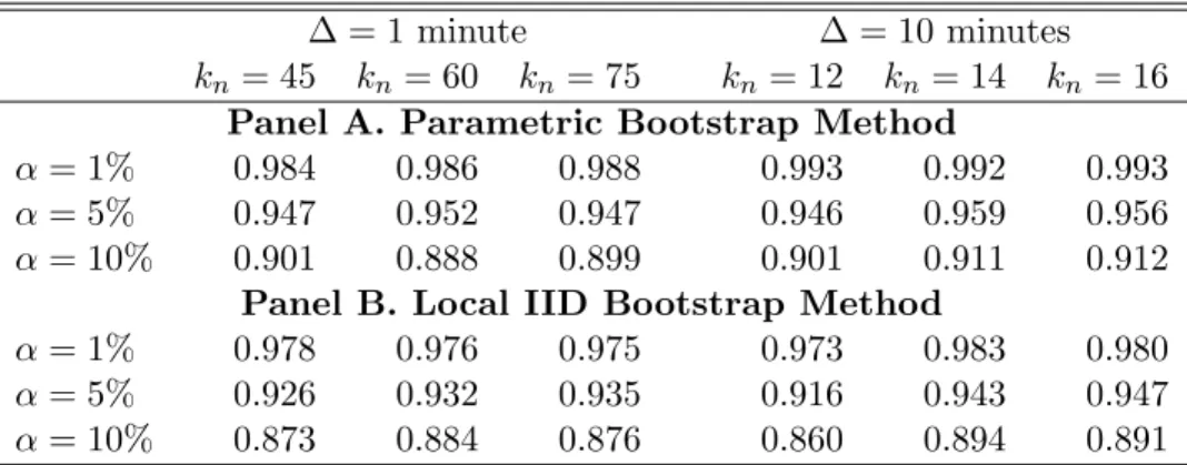
4.1 Monte Carlo coverage probabilities for non-overlapping bootstrap
LIST OF FIGURES
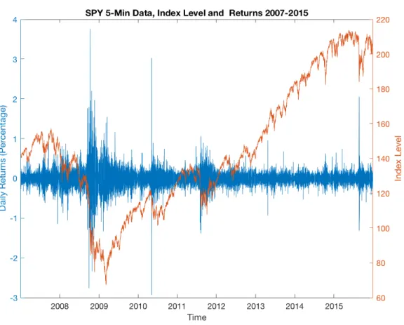
1.1 A typical price path and return . . . 2
6.1 Sampling and Discretization Grid whenδ <∆n . . . 104
6.2 Linear Relation between Market and Individual Stock . . . 118
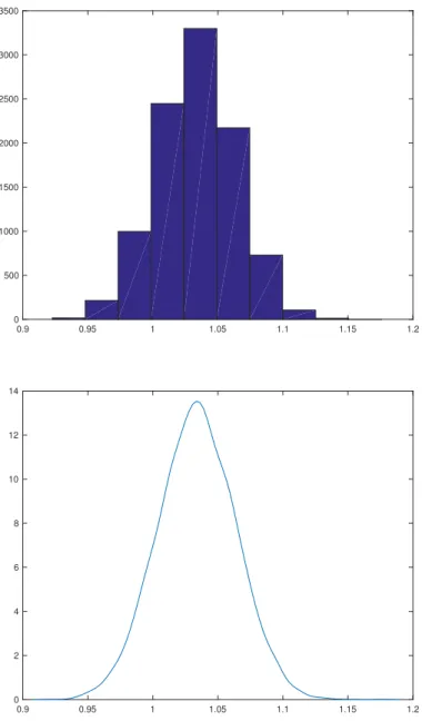
6.3 Sample Distribution of Diffusive Beta . . . 120
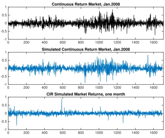
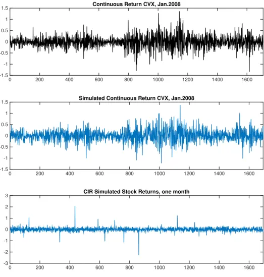
6.4 Simulated Returns for Market . . . 122
CHAPTER 1
Introduction
With the advent of intraday high-frequency data of financial assets since the late 1990s, the research of financial econometrics has entered into a “big data” era. New theoretical techniques using the theory of continuous time stochastic processes has been extensively developed, and new empirical evidence has been documented. In particular, due to its far-reaching applications in various fields such as risk management and option pricing, the study of volatility, which quantitatively measures the uncertainty of prices of financial assets, has drawn substantial attention from researchers and there has been a large amount of literature devoted to this topic. In this Introduction, we offer an overview of the dissertation including the basic set-up, the research questions we are to explore, the main results we have obtained and a direction of future work.
We start with the basic statistical setting. For simplicity, we only consider one-dimensional case in the Introduction and the multivariate setting will be discussed in the fol-lowing chapters. Consider a filtered probability space (Ω,F,(Ft)t≥0,P) satisfying the usual conditions (see e.g., (Jacod and Shiryaev, 2003)), on which are defined a one-dimensional Brownian motionW and a Poisson random measureµonR+×E with deterministic
inten-sityν(dt, dz) =dt⊗λ(dz). HereE is a Polish space. As is usual the case (e.g. (A¨ıt-Sahalia and Jacod, 2014)), we model the logarithm of the price process Xt of a given stock as an
Itˆo semimartingale in the following Grigelionis form:
Xt=x0+
Z t
0
bsds+
Z t
0
σsdWs+ (δ1{kδk≤1})∗(µ−ν)t+ (δ1{kδk>1})∗νt,
where σ is an R−valued predictable (or simply progressively measurable) process on (Ω,F,(Ft)t≥0,P), and δ is a predictable R−valued function on Ω×R+ ×E.
Figure 1.1: A typical price path and return
(a)The price path and returns of SPY from 01/03/2007-12/31/2015, based on 5-min data.
c`adl`ag adapted and hence locally bounded. A typical stock price path can be seen from Figure 1.1.
In finance and econometrics, the processσtis called the spot (or local) volatility of Xt,
and accordingly the spot (local) variance process is defined asct=σt2. Since mathematically
the sign of σt cannot be identified and ct is always nonnegative, it is more straightforward
to consider ct in study, which, abusing the terminology, we still call volatility. Moreover,
sincectis latent (not observable), it can only be recovered by using the data of X sampled
with high-frequency via certain statistical estimation procedures.
interval [(i−1)∆n, i∆n] is given by
∆niX=Xi∆n−X(i−1)∆n.
We consider infill asymptotics where the mesh ∆n of grid of sampling asymptotically tends
to 0 as n→ ∞.
Recall that in a traditional “low frequency” setting, the daily risk has been measured using daily squared returns, see e.g. (Engle, 1982) and (Bollerslev, 1986), or daily range (difference between maximum and minimum within one day), see e.g. (Alizadeh et al., 2002). With the availability of intraday high-frequency data sampled as above, however, a new measure, which is defined as
Z T
0
csds
and calledintegrated volatility, becomes prevailing. A consistent and efficient estimator for the intergrated volatility isrealized volatility, which is defined as the sum of squared intraday returns. Such a method is proposed by (Andersen and Bollerslev, 1999) and popularized by, e.g., (Andersen et al., 2001a) and (Andersen et al., 2003a). More generally, it would be interesting to study the random object of the form
S(g)≡ Z T
0
g(cs)ds,
for some (possibly nonlinear) functiong, which is calledintegrated volatility functional and accommodates many quantities that are related to volatility, including integrated volatility as a special case wheng(x) =x. For other representative examples ofg, see Chapter 3.
The first part of this dissertation, which includes Chapter 3, 4 and 5, focuses on the statistical inference for S(g) under various conditions on the variance process ct and test
function g. More precisely, for given g, the estimator for S(g) can be constructed in two steps: firstly, we nonparametrically recover the spot variance ct over the sampling grid by
2012), Chapter 9 and 13), that is, for any 0≤i≤Nn≡[T /∆n]−kn, let
ˆ ci∆n ≡
1 kn∆n
kn
X
j=1
∆ni+jX21{||∆n
i+jX||≤un},
whereknis a sequence of integers that goes to infinity representing the number of increments
employed in a local window and un determines the truncation threshold for eliminating
jumps in X, see (Mancini, 2001). Next, plugging the estimated spot volatilities into a Riemann approximation framework, the estimator ofS(g) is given by
Sn(g)≡∆n
[T /∆n]−kn
X
i=0
g(ˆci∆n)−
1 kn
g00(ˆci∆n)ˆc2i∆n
, (1.1)
where a higher order bias term is subtracted off.
Assuming that the volatility process follows an Itˆo semimartingale, (Jacod and Rosen-baum, 2013a) shows a CLT (see (4.5) in Chapter 4 below) forSn(g) approximatingS(g) with
rate√∆nprovided test functiongand its derivatives satisfy a polynomial growth condition.
By a local spatialization argument, (Li et al., 2016a) extends the CLT result to the case ofg satisfying a much weaker condition given as Assumption 3.2.1, and (Li and Xiu, 2016) shows an empirical-process-type CLT in a similar setting. However, all these results assume that volatility process is an Itˆo semimartingale, which is actually not able to capture the long memory property of volatility dynamics that has been widely documented in literature, see for example, (Comte and Renault, 1998). In contrast, in Chapter 3 we derive the same CLT result forSn(g) approximatingS(g) with rate
√
∆nfor a larger class of volatility processes:
we assume the volatility process follows a long-memory Itˆo semimartingale (LMIS) which is given by
σt=σ1,t+σ2,t,
whereσ1,tis an Itˆo semimartingale andσ2,tcan be a fractional Brownian motion or a Weiner
Theorem 1.0.1. Under Assumptions 3.1.1-3.4.1, it holds that
1 √
∆n
(Sn(g)−S(g))
L-s
−→ MN(0, V(g)),
where MN(0, V) is a centered mixed normal distribution with conditional variance
V(g)≡2 Z T
0
g0(cs)
2 c2sds.
Here −→L-s denotes stable convergence in law which will be elaborated in Chapter 2. In light of Theorem 1.0.1, inference can be done for S(g): for example, one can con-struct confidence intervals provided that the asymptotic variance V(g) can be consistently estimated, as Corollary 3.7 in (Jacod and Rosenbaum, 2013b). On the other hand, however, a consistent estimator forS(g) is not indispensable to obtain confidence intervals forS(g), as one may turn to bootstrap method.
In Chapter 4, under the assumption that the volatility process σt follows LMIS, we
propose algorithms for constructing confidence intervals forS(g) via both parametric boot-strap method and nonparametric bootboot-strap method. Given bootboot-strap samples of returns D∗n≡ {∆n
iX∗, i= 1, . . . , n}generated either parametrically or nonparametrically, the
boot-strap estimator for S(g) is given by, not surprisingly, an analogue form of (1.1):
Sn(g;Dn∗)≡
kn
n
[n/kn]−1
X
i=0
g(ˆc∗n,i)− 1 kn
g00(ˆc∗n,i)ˆc∗n,i2
,
where
ˆ
c∗n,i= n kn
kn
X
j=1
∆nikn+jX∗2
are bootstrap spot covariance estimators using D∗n. Here we take T = 1,∆n = 1/n and
both ˆc∗n,iand Sn(g;D∗n) are constructed over non-overlapping blocks [ikn/n,(i+ 1)kn/n] for
i∈ In ≡ {0, . . . ,[n/kn]−1}. Then the bootstrap confidence interval of coverage 1−α is
formed as
whereqα/2(Sn(g;D∗n)) andq1−α/2(Sn(g;Dn∗)) are theα/2 and 1−α/2 quantiles ofSn(g;Dn∗)
respectively, computed from a large number of bootstrap repetitions, and
e
Sn(g;Dn) =
kn
n
[n/kn]−1
X
i=0
g(ˆcn,i)
is the uncorrected estimator for S(g). Here we use Dn ≡ {∆niX, i = 1, . . . , n} to denote
the set of original returns, in contrast to its bootstrap counterpart D∗
n. Theoretically, the
asymptotic coverage rate of 1−α is guaranteed by Theorem 1.0.2. In the sequel, we use Zn
L|F
−→Z to denote L(Zn|F)−→ L(ZP |F) for a sequence of random variables (Zn)n≥1 and
Z, namely, the conditional distribution ofZngiven F converges to that ofZ in probability
under Prokhorov metric. Such a mode of convergence in commonly used in the setting of bootstrap, as well as together with stable convergence in law.
Theorem 1.0.2. Suppose the Assumption 3.1.1-3.4.1, it follows that
√ n
Sn(g;Dn∗)−Sen(g;Dn) L|F
−→ MN(0, V(g)),
where
V(g)≡2 Z T
0
g0(cs)
2 c2sds.
Furthermore, we implement Monte Carlo simulation to study the coverage rates of both the parametric and nonparametric bootstrap confidence intervals in finite sample, the results of which validate our theoretical asymptotic result given in Theorem 1.0.2.
Chapter 5 considers a more general form of test function g. We focus on a functional form of the test function g, namely,
g:V ×Θ→R,
where V ⊂ R is the range space of spot volatility, and Θ ⊂ Rdimθ is the space of some
indexing parameterθ. So for each fixed valuect,g(ct,·) is a function over Θ. For example,
information of the volatility process within the time span. See also (Li and Xiu, 2016) Section 3.3 for other econometric applications in this context.
Our goal is to (uniformly) estimate the quantity of the form
S(g;θ)≡ Z T
0
g(cs;θ)ds.
Similarly as in (Li and Xiu, 2016), the proposed estimator is
Sn(g;θ;Dn)≡∆n
[T /∆n]−kn
X
i=0
g(ˆci∆n;θ)−
1 kn
∂c2g(ˆci∆n;θ) ˆc2i∆n
.
Under the assumption that the volatility processσtis an Itˆo semimartingale, plus other
regularity conditions, we are able to obtain the following functional central limit theorem.
Theorem 1.0.3. Suppose Assumption 3.1.1 withσ2= 0, and Assumption 3.2.2. Moreover,
assume g : V ×Θ → R satisfies Assumption 3.2.1 with respect to the first variate and is continuously differentiable with respect to θ ∈Θ, where Θ ⊂Rdimθ is a compact set, with dimθ <∞. Then the sequence∆−n1/2(Sn(g;·;Dn)−S(g;·))of processes convergesF −stably in law under the uniform metric to a process ξ(·) which, conditional on F, is centered Gaussian with covariance function Sg(·,·), where Sg(·,·) is defined as, for any θ, θ0 ∈Θ,
Sg(θ, θ0)≡2
Z T
0
∂cg(cs;θ)∂cg(cs;θ0)c2sds.
Furthermore, in this functional setting we also develop both parametric and nonpara-metric bootstrap algorithms to conduct statistical inference as regard to S(g;·). The al-gorithms are very similar to the ones in Chapter 4 and we provide empirical-process-type asymptotic results to justify both bootstrap algorithms. From an application point of view, such asymptotic results could help constructing (empirical) uniform confidence region for S(g;·).
need to simulate the following diffusion process
dXt=btdt+σtdWt,
where W is Brownian motion. Very often X denotes the log-price of financial asset, say stock, andσ is referred to as the volatility process related toX. The most commonly used method to simulate X is the so-called Euler-Maruyama approximation, which is named after Leonhard Euler and Gisiro Maruyama, and is actually a simple generalization of the Euler method for ordinary differential equations to stochastic differential equations. More precisely, to obtain the value ofX at terminal timeT over a fixed time span [0, T], one uses the recursive equation:
Xτn+1 =Xτn+bτn(τn+1−τn) +στn(Wτn+1−Wτn),
with given discretization grid 0 = τ0 < τ1 < · · · < τN = T. Usually, the equidistant
discretization scheme is used, namely, τi+1−τi = δ for some time step 0 < δ < T. For
a thorough treatment on Euler-Maruyama approximation and its extensions, see (Kloeden and Platen, 1992).
However, to implement such procedure, the values of (bt)t≥0 and (σt)t≥0 have to be
prespecified (or simulated) beforehand, which might not replicate the true world as much as possible, even if the specified values for parameters are claimed to be “calibrated to the real world”.
Alternatively, instead of specifying particular dynamics for (σt)t≥0, we can use estimated
parametric bootstrap confidence interval for integrated volatility functionals (see Algorithm 1 in Chapter 4).
Put it more precisely, we assume that the log-price process follows
dXt =
√ ctdWt
X0 = 0
whereT is the terminal time,cis the variance process andW is one-dimensional Brownian Motion introduced above. In particular, X has neither a drift part nor a jump part. We consider an equally spaced time discretization grid over [0, T] for Euler approximation, i.e., for someδ >0, let
τ0= 0, τi =iδ.
wherei∈ {0,1, . . . ,bT
δc}. At each discretization time pointiδ, the spot volatility estimation
is given by
ˆ ciδ =
1 kn∆n
kn
X
`=1
∆ndiδ
∆ne+`
X 2
.
Then for fixed n and δ, the global Euler approximation with estimated spot volatility is given by the process:
Ytn,δ =
[t/δ]−1
X
i=0
p ˆ
ciδ(Wf(i+1)δ−Wfiδ), 0≤t≤T,
where fW is Brownian motion on the simulation space, which is independent of all the information living in the real world. In particular, forYn,δ to be well-defined, the condition
δ >∆n has to be satisfied.
We derive the theoretical results associated with Yn,δ. The very first thing one should notice is that since in simulation only Wf is available, Yn,δ is a “consistent estimator” for the simulated log-price defined by
e Xt=
Z t
0
√
rather than the true price observed processXt, which has the same distribution asXetunder the no leverage assumption, i.e., the volatility processct and Brownian motionWt, both of
which are defined from the real world, are independent. To derive the convergence rate of Yn,δ approximatingX, we havee
Theorem 1.0.4. Suppose Assumptions 6.2.1 and 6.2.3. Assume further that {ct :t≥ 0}
has sample paths satisfying for any t > s >0,
E|ct−cs|2 ≤K|t−s|2ρ, 0< ρ≤1,
for some constant K. Then it holds for any fixed discretization distance δ∈[∆n, T) that
E sup
0≤t≤T
|Ytn,δ−Xet| !
≤K √1 kn
+ (kn∆n)ρ+δρ+
δlog 2T δ
1
2 !
for some constant K.
From Theorem 1.0.4 we are able to derive the “optimal” simulation scheme in the sense of fastest convergence rate: to make Yn,δ converges to
e
X as fast as possible, one should first takeδn→0 as small as possible, i.e.
δn= ∆n,
which means taking each data sampling point as a discretization point; then we strike balance between statistical error and target error arising from spot volatility estimation, by requiring
kρ+ 1 2
n ∆ρn→β ∈(0,∞),
or equivalently kn∼∆
− ρ
ρ+ 12
n . In this fashion, our “optimal” Euler approximation becomes:
Ytn=
bt/∆nc−1
X
i=0
p ˆ
with convergence rate
E sup
0≤t≤T
|Ytn−Xet| !
≤ K √1 kn
+ kn∆n
ρ
+ ∆ρn+
∆nlog
2T ∆n
12!
∼ ∆
1 2+ 1ρ
n .
Future Work: The results obtained above give us a solid foundation for future work. As for the project of bootstrap inference, we have the following to do
• Consider the over-lapping case, besides the non-overlapping case studied already; • Prove a similar asymptotic result when the volatility process is of the mixed form
considered in Chapter 3.
• Prove a similar asymptotic result when g is a functional, characterized by another indexing parameterθ, as the setting in Chapter 5.
As for the project of Euler method with estimated spot volatility, we can continue the study in both theory and application:
• Theory: An interesting direction to generalize our Euler method with estimated volatility is to take into account the so-called leverage effect, which refers to the negative correlation between volatility and returns. Since the Brownian motion Wf used in simulation is independent of everything in the real world, to create (negative) correlation between the simulated prices and volatility, we need to use the same Wf to regenerate volatility process, which requires to model volatility process as an Itˆo semimartingale as well and estimate the volatility of volatility (vol. of vol.). As one may imagine, the convergence rate in this situation would be even slower than ∆1n/4
as both volatility and vol. of vol. are latent.
• Application: The daily range of a given price process X, defined as the difference between maxXtand minXt within one day, had been a popular measure to quantify
CHAPTER 2
Preliminaries
We start with notation that will be used throughout the paper. For a vectorB, we use Bj to denote its j-th component. For an integer d > 0, Md denotes the space of d×d nonnegative semidefinite matrices. For a matrix A, we use Aij and A| to denote its (i, j) element and transpose, respectively. For a matrix valued process At, the notations Aijt
and A|t are interpreted similarly. For a matrix A ∈ Md and a differentiable function g defined onMd, the first two partial derivatives ofg are denoted as∂jkg(A) =∂g(A)/∂Ajk
and ∂jk,lm2 g(A) =∂2g(A)/∂Ajk∂Alm respectively. For a set B, 1B(·) denotes the indicator
function of setB. The symbol≡indicates equality by definition. ||·||denotes the Frobenius norm. For any two (possibly random) real-valued sequences (an)n≥1 and (bn)n≥1, we write
an=Op(bn) if an/bn is bounded in probability and writean=op(bn) ifan/bnconverges to
0 in probability. All limits are forn→ ∞. We use−→,P −→L and−→L-s to denote convergence
in probability, convergence in law and stable convergence in law, respectively. We useK to denote a generic constant which may vary from line to line.
In this section we give a brief introduce to two important notions that will be used frequently in the rest of dissertation. Section 2.1 introduces Itˆo semimartingale, which is a basic class of stochastic processes commonly used in econometrics and finance. Sec-tion 2.2 discusses the so-called stable convergence in law, which is stronger than the usual convergence in law (or weak convergence).
2.1 Itˆo semimartingale
measures, see (Jacod and Shiryaev, 2003), (Jacod and Protter, 2012) and (A¨ıt-Sahalia and Jacod, 2014). We consider a filtered probability space (Ω,F,(Ft)t≥0,P), where the filtration (Ft)t≥0 satisfies the usual condition as given in (Jacod and Shiryaev, 2003) p.2.
Through-out the paper, all stochastic processes, unless otherwise specified, are assumed to be c`adl`ag adapted and hence locally bounded.
Definition 2.1. (a) A semimartingale is a processXof the formX=X0+M+Awhere
X0 is finite-valued andF0−measurable,M is a local martingale with M0= 0, and A
is a stochastic process of finite variation.
(b) A special semimartingale is a semimartingaleX which admits a decompositionX = X0+M+A as above, with a process A that is predictable.
Given anRd−valued process X, the jump measure associated with X is defined as
µX = X
s>0:∆Xs6=0
(s,∆Xs),
wherea denotes the Dirac measure sitting ata. Then we can rewrite a semimartingale as
Xt=X0+A0t+Mt+
X
s≤t
∆Xs1{k∆Xsk>1}
where M0 = A00 = 0 and A0 is of finite variation and M is a local martingale. Then the
semimartingale A0+M by construction has jumps of size always smaller than 1. Hence by Lemma 4.24 in (Jacod and Shiryaev, 2003), A0+M is special and we can write
A0+M =B+N,
where N0 = B0 = 0 and N is a local martingale and B is a predictable process of finite
variation.
Definition 2.2. The characteristic of aRd−valued semimartingaleX is the following triple (B, C, ν):
(ii) C= (Cij)1≤i,j≤dis the quadratic variation of the continuous local martingale partXc
of X, that is, Cij =hXi,c, Xj,ci;
(iii) ν is the predictable compensating measure of the jump measure µX of X.
One should note that the characteristic triple does NOT characterize the law of the process except for special cases. An important special case of semimartingale is Levy process, the characteristic triple of which is
Bt(ω) =bt, Ct(ω) =ct, ν(ω, dt, dx) =dt⊗F(dx),
which are not random actually. For a general treatment of L´evy process, see (Bertoin, 1998).
In financial modelling, it is common to use a special class of semimartingales, but which is also a direct extension of L´evy process:
Definition 2.3. A Rd−valued semimartingaleX is an Itˆo semimartingale if its character-istic (B, C, ν) are absolutely continuous with respect to the Lebesgue measure, in the sense that
Bt=
Z t
0
bsds, Ct=
Z t
0
csds, ν(dt, dx) =dtFt(dx),
where b = (bt) is an Rd−valued process, c = (ct) is a process with values in Md, and
Ft=Ft(ω, dx) is for each (ω, t) a measure on Rd.
Now we come to give a fundamental representation theorem for Itˆo semimartingale, which is usually referred to as the Grigelionis form of Itˆo semimartingale. The following theorem is Theorem 2.1.2 in (Jacod and Protter, 2012). Letd0 be an arbitrary integer with d0 ≥ d, E be a Polish space with a σ−finite measure λ having no atom, and q(dt, dx) = dt⊗λ(dx).
Theorem 2.1.1. Let X be a d−dimensional Itˆo semimartingale on the space
(Ω,F,(Ft)t≥0,P), with characteristics (B, C, ν). There is a very good filtered extension
Poisson random measure p onR+×E with L´evy measureλ, such that
Xt=x0+
Z t
0
bsds+
Z t
0
σsdWs+ (δ1{kδk≤1})∗(p−q)t+ (δ1{kδk>1})∗pt, (2.1)
and where σ is an Rd⊗Rd 0
−valued predictable (or simply progressively measurable) on (Ω,F,(Ft)t≥0,P), andδ is a predictable Rd−valued function on Ω×R+×E.
For a more detailed description of extension of probability space, see (Jacod and Protter, 2012) p.36-37. The point of Theorem 2.1.1 is that any d−dimensional Itˆo semimartingale can be expressed in terms of a Brownian motion and a Poisson random measure, and in fact, (2.1) can be used as the definition for Itˆo semimartingales, up to extending the space. Itˆo semimartingales of form (2.1) have been widely used in modelling prices of financial assets for various reasons. At first, it has been widely known that the prices of financial assets, say stocks, have jumps, which for example occurs when there is significant macroeco-nomic announcements. Although we consider Poisson random measure with a compensator of product form, dt⊗λ(dx), which is time-homogeneous, the whole jump part in (2.1) is actually time-inhomogeneous since the jump size function δ is random and time-varying. As a consequence the jump part of stock price is driven by a very general class of processes. As for continuous part, the drift part captures the persistence in the process, and also rep-resents the compensation for risk and time, while the continuous martingale part given as a stochastic integral models the small moves.
In fact, as (Back, 1991) points out, special semimartingale appears to be the most general concept of a gains process for which the notion of a local risk premium can be well-defined. On the other hand, (Barndorff-Nielsen and Shephard, 2004a) (Remark 1) and (Barndorff-Nielsen et al., 2006) (Remarks 3) demonstrate the generality of the continuous (local) martingale part Rt
0σsdWs in (2.1). More precisely, by a representation theorem of
local martingale as stochastic integral (e.g., (Karatzas and Shreve, 1991) p.170-172), all continuous local martingales with absolutely continuous quadratic variation can be written in the form of R0tσ˜sdWs for some process ˜σt. Using the Dambis-Dubins-Schwartz theorem,
absolutely continuous quadratic variation. Thus the form of continuous (local) martingale part we consider here is only slightly smaller the class of general continuous local martingale.
2.2 Stable convergence in law
In this subsection we introduce the notion of stable convergence in law, which is stronger than the usual convergence in law or weak convergence. We first review the definition of the latter for illustrative purpose.
Let E be a Polish space, with Borel σ-field E. Let {Zn} be a sequence of E-valued random variables, allowing each of them defined on its own probability space (Ωn,Fn,Pn). Definition 2.4. We say that Zn converges in law if there is a probability measure µ on
(E,E) such that
E(f(Zn))−→
Z
f(x)µ(dx).
for all (Lipschitz) continuous bounded functions f on E.
Usually, one could “realize” the limit as aE-valued random variable Z on some proba-bility space (Ω,F,P), then the above convergence reads as
E(f(Zn))−→E(f(Z)).
However, the usual convergence in law defined as above may not be enough in the area of financial econometrics. As one can see, quite often we will be in the following scenario: we need to estimate some (multivariate) parameterθ and we propose a sequence of consistent estimators ˆθn. We are able to show a central limit theorem with certain convergence rate,
say√nand mixed normal limiting distribution, namely, √
nθˆn−θ
L
−→ N(0,Σ).
distribution. However, this may not be achieved even if Σ can be consistently estimated, as
Zn
L
−→Z, Yn−→P Y
do NOT in general imply
(Zn, Yn)
L
−→(Z, Y),
the only exception being Y is a constant, which is case of the so-called Slutsky Theorem. We hence need a stronger version of convergence in law to make sure the joint convergence (Zn, Yn)
L
−→(Z, Y),still holds even ifY is random.
We require E-valued sequence {Zn} of random variables to be defined on the same probability space (Ω,F,P).
Definition 2.5. We say that Zn stably converges in law if there is a probability measure
η on the product space (Ω×E,F ⊗ E), such that η(A×E) =P(A) for all A∈ F and
E(Y f(Zn))−→
Z
Y(ω)f(x)η(dω, dx)
for all bounded (Lipschitz) continuous functions f onE and all bounded random variables Y on (Ω,F).
As before, we can “realize” the limitZon an (arbitrary) extension (Ω,e F,e fP) of (Ω,F,P), then the stable convergence in law above can be written as
E(f(Zn))−→E˜(Y f(Z)),
providedPe(A∩ {Z ∈B}) =η(A×B) for allA∈ F andB ∈ E. Then we sayZn converges stably to Z, denoted by
Zn
L−s
−→Z.
By definition, it immediately follows that stable convergence in law implies convergence in law. Moreover, we do have the desired property
Zn
L−s
−→Z, Yn−→P Y =⇒ (Zn, Yn)
L−s
In fact, stable convergence in law is very much like convergence in probability: when the limiting variableZ is defined on the same space Ω as all Zn, it follows that
Zn
L−s
−→Z ⇐⇒ Zn−→P Z.
CHAPTER 3
Efficient Estimation of Integrated Volatility Functionals with General Volatility Dynamics
3.1 Setting
We start with introducing the formal setup for our analysis. Consider a complete filtered probability space (Ω,F,(Ft)t≥0,P). Throughout the chapter, all stochastic processes, unless otherwise specified, are assumed to be c`adl`ag adapted and hence locally bounded. Our basic assumptions of underlying processes are collected in Assumption 3.1.1.
Assumption 3.1.1. For some constant r ∈ [0,1), and a sequence of a sequence (τm)m≥1
of stopping times increasing to ∞, we have
(i) The process Xt is ad−dimensional Itˆo semimartingale with the form
Xt=x0+
Z t
0
bsds+
Z t
0
σsdWs+Jt, Jt=
X
s≤t
∆Xs=
Z t
0
Z
R
δ(s, z)µ(ds, dz), (3.1)
where the driftbtisd−dimensional; the spot volatility processσtisRd⊗Rdvalued;Wt is a d−dimensional Brownian motion; µis a Poisson random measure onR+×E for
an auxiliary Polish spaceE with the deterministic intensity measure ν(dt, dz) =dt⊗ λ(dz)for someσ−finite measureλonE;δ: Ω×R+×E→Rdis a predictable function.
Moreover, there are a sequence (Jm)m≥1 of nonnegative λ−integrable deterministic
functions onE such that ||δ(ω, t, z)||r∧1≤J
m(z) for all t≤τm(ω) and z∈E. (ii) The spot volatility process σt is of the form
Moreover, both σ1,t and c1,t=σ1,tσ|1,t ∈ Md are Itˆo semimartingales of the following Grigelionis form
σ1,t = σ1,0+
Z t
0
b(σ1)
s ds+
Z t
0
σ(σ1)
s dWs+
Z t
0
Z
R
δ(σ1)(s, z)1
{||δ(σ1)(s,z)||>1}µ(ds, dz) +
Z t
0
Z
R
δ(σ1)(s, z)1
{||δ(σ1)(s,z)||≤1}(µ−ν)(ds, dz)
c1,t = c1,0+
Z t
0
b(c1)
s ds+
Z t
0
σ(c1)
s dWs+
Z t
0
Z
R
δ(c1)(s, z)1
{||δ(c1)(s,z)||>1}µ(ds, dz)
+ Z t
0
Z
R
δ(c1)(s, z)1
{||δ(c1)(s,z)||≤1}(µ−ν)(ds, dz)
where W andµare the same as in (3.1); b(σ1), b(c1), δ(σ1), δ(c1) ared×d−dimensional
andσ(σ1), σ(c1)ared×d×d−dimensional; δ(σ1), δ(c1)are predictable functions such that
for a sequence of nonnegative λ-integrable functions J˜m on E, ||δ(σ1)(ω, t, z)||2∧1≤
˜
Jm(z) and ||δ(c1)(ω, t, z)||2∧1≤J˜m(z) for allt≤τm(ω) and z∈E. On the other hand,σ2,t is a stochastic process satisfying, for some >0,
E ||σ2,t−σ2,s||2
≤K(t−s)1+2 (3.3)
and long-memory process, in the sequel we refer to model (3.2) as the long-memory Itˆo semimartingale (LMIS) volatility model.
On the technical level, as long asσ1is an Itˆo semimartingale,c1is also an Itˆo
semimartin-gale by Itˆo’s formula. The processes b(c1), σ(c1) and δ(c1) can be expressed as deterministic functions of σ1, b(σ1), σ(σ1) and δ(σ1), but we do not need this here. On the other hand,
as far as the conditions imposed on the process σ2 is concerned, since σ2 may not be a
martingale any more (e.g., when σ2 is fractional Brownian motion), the conditional
expec-tation ofσ2,t−σ2,s givenFs could be difficult to compute and hence complicates the proof
of Theorem 3.4.1 below. This is the reason why more smoothness on the second moment (3.3) is needed, which can be seen as compensation for the loss of martingale property.
Now we state the statistical setting in this chapter. At stage n, we assume that the processX is sampled at timesi∆nfor some time step ∆n, for 0≤i≤n≡ bT /∆nc, within
thefixed time interval [0, T]. For any process Y, the increments ofY are denoted by
∆niY ≡Yi∆n−Y(i−1)∆n, i= 1, . . . , n. (3.4)
Below, we consider an infill asymptotic setting, that is, ∆n→0 as n→ ∞.
3.2 Integrated volatility functional
With model (3.1), the spot (co)variance process ofX is given byc=σσ|, which is also Md-valued. The (random) object of interest considered in this chapter is the integrated volatility functional of the form
S(g)≡ Z T
0
g(cs)ds, (3.5)
for some (possibly nonlinear) test function g : Md → R, which is assumed to satisfy the following assumption. Below, for a compact set K ⊂ Md and > 0, we denote the -enlargement aboutK by
K ≡ {M ∈ M d: inf
Assumption 3.2.1. There exist a localizing sequence of stopping times (τm)m≥1 and a
sequence of convex compact subsetsKm ⊆ Mdsuch thatct∈ Kmfort≤τm andg∈ C3(Km), the space of three times continuously differentiable functions on K
m for some >0.
Assumption 3.2.1 is easily verified in specific setting, which in particular holds, in one-dimensional case, forg(c) = log(c) or√c, provided that bothctand 1/ctare locally bounded
withKm being compact intervals on (0,∞).
Many quantities of interests in finance and econometrics can be written in the form of (3.5), with Assumption 3.2.1 satisfied. For example, whencis scalar,g(x) =x corresponds to the so-called integrated volatility S(g) =R0T ctdt, which has been a popular measure of
volatility in high-frequency setting, see (Andersen and Bollerslev, 1999), (Andersen et al., 2001b) and (Andersen et al., 2003b). Moreover, g(x) = x2 corresponds to the integrated quarticity, which is the (half of) asymptotic variance when using realized volatility to ap-proximate integrated volatility. The more generally definedpower variation S(g) =RT
0 c
p tdt
for some p > 0 is associated with polynomial test function g(x) = xp, see for example, (Barndorff-Nielsen and Shephard, 2003), (Barndorff-Nielsen and Shephard, 2004b) and (Ja-cod, 2008). In bivariate case, the beta for the diffusive movement of the stock with respect to the market is given byβt≡c12,t/c11,t, where the market and the stock are labelled by 1 and
2 respectively, with the test function being g(A) =A12,t/A11,t for A∈ M2, see (Mykland
and Zhang, 2009). Moreover, the idiosyncratic spot covariance of the stock can thus be ex-pressed asc22,t−β2tc11,t =c22,t−c212,t/c11,t, with test functiong(A) =A22,t−A212,t/A11,t, see
returns (see (Jacod and Protter, 2012), Chapter 9 and 13), that is, for any 0≤i≤Nn ≡
[T /∆n]−kn, let
ˆ
clmi∆n ≡ 1 kn∆n
kn
X
j=1
∆ni+jXl∆ni+jXm1{||∆n
i+jX||≤un}
where 1≤l, m≤d,knis a sequence of integers that goes to infinity representing the number
of increments employed in a local window and un determines the truncation threshold for
eliminating jumps inX, see (Mancini, 2001) and (Mancini, 2009). If X is continuous, then there is no need to truncate in forming ˆc by taking un = ∞ . The conditions on tuning
parameters kn and un are collected in Assumption 3.2.2. We note that the study of spot
covariance estimation dates back to (Foster and Nelson, 1996), which features a continuous setting; one can also see (A¨ıt-Sahalia and Jacod, 2014) on this topic in a more general setting.
Assumption 3.2.2. kn∼∆−nγ and un∼∆$n for some constants γ and$ satisfying
r 2 ∨
1 3 < γ <
1 2,
1−γ
2−r ≤$ < 1 2.
In particular, kn∆n→0 and kn2∆n→ ∞.
We then define the estimator for S(g) as
Sn(g)≡∆n
[T /∆n]−kn
X
i=0
g(ˆci∆n)− 1 2kn
d
X
j,k,l,m=1
∂jk,lm2 g(ˆci∆n)×(ˆcjli∆nˆc
km i∆n+ ˆc
jm i∆ncˆ
kl i∆n)
(3.6)
Assuming that the volatility process is an Itˆo semimartingale, (Jacod and Rosenbaum, 2013a) shows a CLT forSn(g) approximating S(g) with rate
√
∆nprovided test function g
(and its derivative) satisfy a certain growth condition. (Li et al., 2016a) extends the CLT result to the case of g only satisfying Assumption 3.2.1, and (Li and Xiu, 2016) shows an empirical-process-type CLT in a similar setting, while both papers still assuming volatility process is an Itˆo semimartingale. In contrast, in this chapter we want to derive an associated CLT for Sn(g) approximating S(g) with convergence rate
√
variance as in the aforementioned papers for a larger class of volatility processes given as LMIS (3.2).
3.3 Examples
In this section we provides some concrete examples for the processσ2 satisfying certain
regularity conditions introduced in Assumption 3.1.1. We begin with fractional Brownian motion in Section 3.3.1, and then proceed to Wiener integrals with respect to fractional Brownian motion in Section 3.3.2.
3.3.1 Fractional Brownian motion Fractional Brownian motion (fBm) (BH
t )t≥0 with Hurst indexH ∈(0,1) is a centered
Gaussian process with the covariance function
E(BtHBHs ) =
1 2(s
2H +t2H − |t−s|2H),
where for simplification we assume B0H = 0. The process was introduced by (Kolmogorov, 1940), followed by pioneering works including (Hurst, 1951), (Hurst, 1956) and (Mandelbrot, 1983). Fractional Brownian motion has been widely used in hydrology, engineering and finance. When H= 12, the process reduces to the usual standard Brownian motion.
For a more comprehensive description of fractional Brownian motion, see, e.g., (Duncan et al., 2000), (Nualart, 2005), (Nualart, 2006) and (Mishura, 2008). We briefly summarize some important properties of fractional Brownian motion below:
1. Self-similarity: for any a >0, {BH
au, u∈R} d
=aH{BH
u , u∈R},where d
= denotes the equality in any finite-dimensional distributions. This property can be regarded as a “fractal property” in probability.
2. Stationary increments and moment estimates: From definition it follows that the increment of BH over a finite time interval [s, t] is normally distributed with mean zero and variance
E
BtH −BsH2
Indeed, for any integer k≥1, we have
E
BtH −BsH2k
= (2k)! k!2k|t−s|
2Hk.
Then by Kolmogorov’s continuity criterion (e.g. (Revuz and Yor, 1999), Theorem 2.1 in Chapter 1),BH has a version whose sample paths areγ−H¨older continuous for any γ < H.
More generally (see, e.g., Corollary 3.11 in (Duncan et al., 2000)), for any α > 1, there is aCα<∞ such that
EBtH −BsH
α
≤Cα|t−s|αH. (3.7)
3. Long memory property when H > 12: Let r(n) ≡ Cov B1H, BnH+1−BnH be the autocovariance function, then ifH >1/2, we have P∞
n=1r(n) =∞, in which case we
call that the fractional Brownian motion exhibits long-range dependence.
4. Non-semimartingale: BH is not a semimartingale whenH 6= 1/2. This can be proved by studying the p−th variation of BH, see, e.g., Proposition 7.1.1 of (Pipiras and Taqqu, 2016).
5. Prediction formula: The conditional expectation of BtH given the past information is given as (3.8). This is first proved by (Gripenberg and Norros, 1996) for the case H >1/2, and extended toH∈(0,1/2) by (Pipiras and Taqqu, 2001) (Theorem 7.1). To state the result more easily, let κ = H −1/2, then for any 0 ≤ s ≤ t ≤ T and κ∈(−1/2,1/2), we have
E Btκ
Bvκ, v∈[0, s]
=Bsκ+ Z s
0
Ψκ(s, t, v)dBvκ, (3.8)
where forv∈(0, t),
Ψκ(s, t, v) = sin(πκ) π v
−κ(s−v)−κZ t s
We note that the function Ψκ(s, t, v) is related to the so-called Appell’s hypergeometric function, see e.g., Remark 6.4.5 in (Pipiras and Taqqu, 2016).
(Comte and Renault, 1996) and (Comte and Renault, 1998) for the first time introduced fractional Brownian motion to modelling the price and volatility processes of financial as-sets. In fact, the long memory property of volatility processes has been documented in economics and finance for a long time. As one may expect, it is the long range dependence property described above that makes fractional Brownian motion an ideal stochastic process to capture such features exhibited by volatility. As a consequence, in the remainder of this chapter we will only consider fractional Brownian motion BH withH >1/2, as well as its continuous version. Then BH satisfies the conditions imposed on σ
2 in Assumption 3.1.1. Remark 3.3.1. On the technical level, sinceBH is not a semimartingale, and also in light of the prediction formula (3.8), it would be rather hard to verify the estimate
|E BtH+s−BtHFt
| ≤Ks
for some constantK, which is always true for any Itˆo semimartingale under certain bound-edness conditions (see Lemma 2 in the Proofs). The lack of such an estimate complicates the proof of Theorem 3.4.1 whenσ2=BH. However, the difficulty is overcome by the more
smoothnessBH provides as shown in (3.7) whenH >1/2.
3.3.2 Wiener integrals w.r.t. fractional Brownian motion
In this example, we focus on the integral over an finite interval [0, T] of the form
Z t
0
f(u)dBuH, 0≤t≤T, (3.9)
deterministic function, (3.9) can be defined in a relatively easier fashion, in which case (3.9) is called fractional Wiener integral.
The integration with respect to general Gaussian processes has been studied for a long time and we refer readers to (Huang and Cambanis, 1978) for an extensive presentation. (Pipiras and Taqqu, 2000) discussed some related questions of Wiener integral of determin-istic integrand w.r.t fractional Brownian motion over the real line, and (Pipiras and Taqqu, 2000) discussed that of over a finite interval, which is the case of (3.9) we consider here. The basic idea is to define (3.9) first withf being elementary(step) functions, and then extend the definition to some bigger classes off in theL2(Ω) sense using isometry. Indeed, when H >1/2, (3.9) can be defined for each of the following four increasing classes of integrands:
L2[0, T]⊂L1/H[0, T]⊂ |Λ|κT ⊂ΛκT,
whereκ=H−1/2 and
ΛκT ≡
f : [0, T]→Rsuch that Z T
0
[s−κ(ITκ−uκf(u))(s)]2ds <∞
,
|Λ|κT ≡
f : [0, T]→Rsuch that Z T
0
Z T
0
|f(u)||f(v)||u−v|2κ−1dudv <∞
.
Here ITκ− is (right-sided) fractional integral operator of orderκ defined as
(ITκ−f)(s) = 1 Γ(κ)
Z T
s
f(u)(u−s)κ−1du, s∈(0, T), f ∈L1[0, T].
For definition of (3.9) for each specific class of integrands, see (Pipiras and Taqqu, 2001) and references therein. For our purpose, it would be sufficient to consider the spaceL1/H[0, T], as seen from the properties of (3.9) listed below. Moreover, as the theory of fractional Brownian motion is closed related to fractional integrals and fractional derivatives, we refer readers to (Samko and Marichev, 1993) for a comprehensive treatment on this topic.
When H >1/2 (or equivalent κ >0), (3.9) has the following properties:
1. Continuity: As explained in (Mishura, 2008), Section 1.11, when f ∈L1/H[0, T], the process
n Rt
0f(u)dB
H u
o
2. Moment estimates: For anyp≥1,0≤a < b≤ ∞, define
kfkLp(a,b) ≡
Z b a
|f(u)|pdu 1/p
.
As proved in Theorem 1.1 in (M´emin et al., 2001), there exists a constant c(H, α) such that for every α >0 and for every a, bwith 0≤a < b <∞, we have
E
Z b
a
f(u)dBuH
α!
≤c(H, α)kfkαL1/H(a,b). (3.10)
3. Prediction formula: Similar to (3.8), for any 0≤s < t≤T and f ∈ΛκT, we have
E Z t
0
f(v)dBvκ
Bvκ, v∈[0, s]
= Z s
0
f(v)dBκv + Z s
0
Ψκf(s, t, v)dBvκ, (3.11)
where forv∈(0, t),
Ψκf(s, t, v) = sin(πκ) π v
−κ(s−v)−κZ t s
zκ(z−s)κ
z−v f(z)dz.
(3.11) is proved in Lemma 1 of (Duncan, 2006). One can see (Fink et al., 2013) for derivation of conditional variance, .
By moment estimates (3.10), iff is uniformly bounded from above by some constantM >0 (as in Assumption 3.5.1 in the Proofs), we have
E
Z b
a
f(u)dBuH
α!
≤c(H, α)kfkαL1/H(a,b)≡
Z b a
|f(u)|1/Hdu Hα
≤c(H, α)Mα(b−a)Hα,
which is the RHS of (3.7). Therefore, together with the continuity in time, the process n
Rt
0f(u)dB
H u
o
0≤t≤T satisfies the conditions imposed onσ2.
3.4 Results
Assumption 3.4.1. Assume > 2(1γ−γ).
Under Assumption 3.4.1, it holds that k1+n ∆n → 0, which plays an important role in the proof of Theorem 3.4.1. In light of Assumption 3.2.2, Assumption 3.4.1 implies that > 1/4, which in the case of fractional Brownian motion corresponds to the Hurst parameterH >3/4. Such a requirement is consistent with the empirical results documented in (Comte and Renault, 1998), (Andersen and Bollerslev, 1997), (Andersen et al., 2001b) and (Bollerslev et al., 2013). In particular, those papers estimate the fractional parameter of the underlying volatility process under both low frequency and high frequency settings, and all of the estimated fractional parameters have a value larger than 0.25.
Now we state our main result.
Theorem 3.4.1. Under Assumptions 3.1.1-3.4.1, it holds that
1 √
∆n
(Sn(g)−S(g))
L-s
−→ MN(0, V(g)),
where MN(0, V) is a centered mixed normal distribution with conditional variance
V(g) =
d
X
j,k,l,m=1
Z T
0
∂jkg(cs)∂lmg(cs)
cjlsckms +cjms ckls
ds.
We give some comments as follows on Theorem 3.4.1.
1. Theorem 3.4.1 extends the results in (Jacod and Rosenbaum, 2013a), (Li et al., 2016a) and (Li and Xiu, 2016) by establishing the asymptotic distribution ofSn(g) under the
LMIS volatility dynamics. In particular, in the absence of the long-memory component σ2, Theorem 3.4.1 coincides with those in prior work. Since both the convergence rate
and the asymptotic variance remain the same as shown in those papers, the estimator Sn(g) is still efficient in the sense of (Jacod and Rosenbaum, 2013a) under the more
general LMIS volatility dynamics.
2. The “cost” of including the long-memory component is that we need an additional upper bound for the divergence rate of the local window sizekn, that is,γ <2/(1+2).
memory. In the extreme case with = 1/2 (i.e., σ2 has locally Lipschitz path under
the L2-norm), this restriction is absent, because σ2 then behaves essentially like a
drift term.
3. As already pointed previously, the condition (3.4.1) implicitly imposes a restriction on , that is, > 1/4. In other words, σ2 is H¨older-continuous under the L2-norm
with an index at least 3/4, which shows an apparent discrepancy relative to the 1/2 H¨older continuity of the Itˆo semimartingale component. This “gap” arises as a compensation for the lack of martingale property in the long-memory component, whereas the martingale property is heavily exploited in previous work based on the Itˆo semimartingale volatility dynamics. The proofs in the more general LMIS framework thus contains nontrivial additional complications.
4. Last but not least, as far as the application of Theorem 3.4.1 is concerned, one can conduct statistical inference, constructing confidence interval for example, for S(g). More specifically, as shown in (Jacod and Rosenbaum, 2013a), a consistent estimator for the asymptotic varianceV(g) is given by
e
Sn(¯h,Dn)≡∆n
[T /∆n]−kn
X
i=0
¯ h(ˆci∆n),
where ¯h(x) ≡ Pd
j,k,l,m=1∂jkg(x)∂lmg(x) xjlxkm+xjmxkl
. In particular, Sen(¯h,Dn) is robust to the long memory assumption of volatility. Then it follows that
e
Sn(¯h,Dn)−→P V(g),
and hence
Sn(g,Dn)−S(g)
q
∆nSen(¯h,Dn) L-s
−→ N(0,1),
3.5 Proofs
Throughout this section, we useK to denote a generic constant that may change from line to line; we sometimes emphasize the dependence of this constant on some parameterq by writingKq. Recall thatNn≡[T /∆n]−kn, we writePi for
PNn
i=0 for simplicity.
3.5.1 Preliminaries
By a standard localization procedure (see Lemma 4.4.9 in (Jacod and Protter, 2012)), it is enough to show Theorem 3.4.1 under a stronger version of Assumption 3.1.1.
Assumption 3.5.1. We have Assumption 3.1.1. The process σ takes value in a convex
compact set of Md. Moreover, the processes b, b(σ1), b(c1) and σ(σ1), σ(c1) are bounded and
there is a bounded λ−integrable function J :E →R, such that for all ω ∈Ω, t∈[0, T]and z∈E we have ||δ(ω, t, z)||r ≤J(z) and||δ(σ1)(ω, t, z)||2∨ ||δ(σ1)(ω, t, z)||2≤J(z).
In the following analysis, it would be much more convenient to consider the continuous part of the processXt defined by
Xt0= Z t
0
bsds+
Z t
0
σsdWs, 0≤t ≤T.
Accordingly, define for eachi= 0,1, . . . , Nn,
ˆ
c0i∆n = 1 kn∆n
kn
X
j=1
∆ni+jX0∆ni+jX0|.
Then we introduce the following notations that will be used throughout the Proofs, most of which are analogues to those used in (Jacod and Rosenbaum, 2013a):
αn,i ≡ ∆niX0∆niX0|−c(i−1)∆n∆n
˜
cn,i ≡ ˆc0i∆n−ci∆n =
1 kn∆n
kn
X
j=1
With any processZ we associate the variables
ηt,s(Z) ≡ sup v∈(0,s]
||Zt+v−Zt||2
ηi,jn (Z) ≡ q
E η(i−1)∆n,j∆n(Z)
F(i−1)∆n
ηni(Z) ≡ ηi,kn n(Z)
and we recall Lemma 3.1 of (Jacod and Rosenbaum, 2013b).
Lemma 3.5.1. For all t > 0 and all bounded c`adl`ag processes Z, we have
∆nE(P[it/=1∆n]ηin(Z)) → 0, and for all j, k such that j + k ≤ kn, we have
E
ηni+j,k(Z)|F(i−1)∆n
≤ηni(Z).
We collect some standard estimates for Itˆo semimartingale in the following lemma, the proof of which depends heavily on the decomposition of ct−cs for 0≤s < t≤T,
ct−cs = (σ1,t+σ2,t)(σ1,t+σ2,t)|−(σ1,s+σ2,s)(σ1,s+σ2,s)|
= (σ1,tσ1|,t−σ1,sσ1|,s) + (σ2,tσ|2,t−σ2,sσ2|,s) + (σ1,tσ2|,t+σ2,tσ1|,t−σ1,sσ|2,s−σ2,sσ1|,s)
= c1,t−c1,s+c2,t−c2,s+ (σ1,t−σ1,s)σ2|,s+σ1,t(σ|2,t−σ |
2,s). (3.12)
+σ2,s(σ1|,t−σ|1,s) + (σ2,t−σ2,s)σ1|,t
Notice that the third and fourth terms are transposes of the fifth and sixth terms, respec-tively. Moreover, we have for i= 1,2 (in fact we only needi= 2 below, as c1,t is itself an
Itˆo semimartingale by Itˆo’s lemma),
ci,t−ci,s = σi,tσ|i,t−σi,sσi,s|
= (σi,t−σi,s)σi,t| +σi,s(σi,t| −σ|i,s) (3.13)
One will see both decompositions (3.12) and (3.13) will be repeatedly used in the sequel.
(1) for anys, t≥0 and q≥0,
E sup
v∈[0,s]
||Xt0+v−Xt0||qFt !
≤ Kqsq/2,
||E Xt0+s−Xt0Ft
|| ≤ Ks, E sup
v∈[0,s]
||σ1,t+v−σ1,t||q
Ft
!
≤ Kqs1∧q/2,
||E σ1,t+s−σ1,t
Ft
|| ≤ Ks, E sup
v∈[0,s]
||c1,t+v−c1,t||q
Ft
!
≤ Kqs1∧q/2,
||E c1,t+s−c1,t
Ft
|| ≤ Ks.
(2) Let c2,t=σ2,tσ2|,t, for any s, t≥0,
E(||σ2,t−σ2,s||) ≤ K(t−s)1/2+
E(||c2,t+s−c2,t||q) ≤ KE(||σ2,t+s−σ2,t||q), q = 1,2,3,4
||E ct+s−ct
Ft
|| ≤ K ||E c1,t+s−c1,t
Ft
||+||E σ1,t+s−σ1,t
Ft
|| +E ||σ2,t+s−σ2,t||
Ft
E(||ct+s−ct||q) ≤ K(E(||σ1,t+s−σ1,t||q) +E(||σ2,t+s−σ2,t||q)), q= 1,2,3,4.
In particular, as one can see from the proof of the third estimate in (2), it would suffice to
consider σ1,t−σ1,s and σ2,t−σ2,s when it comes to the difference ct−cs in the sequel. Proof. The estimates in (1) follow from (4.3) in (Jacod and Rosenbaum, 2013a), as X0 has no jump part and bothσ1,t and c1,t are Itˆo semimartingales.
For part (2), the first estimate is implied by (3.3). For q = 1,2,3,4, by (3.13) and the fact that for any matrix A,||A||=||A||| and thatσ
2 is bounded, it follows
E(||c2,t+s−c2,t||q) ≤ E
||(σ2,t+s−σ2,t)σ2|,t+s+σ2,t(σ2|,t+s−σ|2,t)||q
≤ KE
||(σ2,t+s−σ2,t)σ2|,t+s||q
+KE
||σ2,t(σ|2,t+s−σ|2,t)||q
Hence the second estimate is proved. For the third one, by (3.12)
||E ct+s−ct
Ft
|| = ||E(c1,t+s−c1,t+c2,t+s−c2,t
+(σ1,t+s−σ1,t)σ2|,t+σ1,t+s(σ2|,t+s−σ|2,t)
+σ2,t(σ|1,t+s−σ |
1,t) + (σ2,t+s−σ2,t)σ1|,t+s
Ft
|| ≤ ||E c1,t+s−c1,t
Ft
||+||E
(σ1,t+s−σ1,t)σ|2,t
Ft
|| +||Eσ2,t(σ1|,t+s−σ
| 1,t)
Ft
||+||E c2,t+s−c2,t
Ft
|| +||Eσ1,t+s(σ2|,t+s−σ2|,t)
Ft
||+||E(σ2,t+s−σ2,t)σ1|,t+s
Ft
|| = ||E c1,t+s−c1,t
Ft
||+||E (σ1,t+s−σ1,t)
Ft
σ2|,t|| +||σ2,tE(σ1|,t+s−σ|1,t)Ft
||+||E c2,t+s−c2,t
Ft || +||E
σ1,t+s(σ2|,t+s−σ2|,t)
Ft
||+||E
σ2,t+s−σ2,tσ|1,t+s
Ft
|| ≤ K ||E c1,t+s−c1,t
Ft
||+K||E (σ1,t+s−σ1,t)
Ft
|| +K E ||c2,t+s−c2,t||
Ft
+E ||σ2,t+s−σ2,t||
Ft
≤ K ||E c1,t+s−c1,t
Ft
||+||E σ1,t+s−σ1,t
Ft
|| +E ||σ2,t+s−σ2,t||
Ft
,
as desired.
As for the last estimate, by (3.15) and the fact thatc1, σ1 and σ2 are all bounded,
E(||ct+s−ct||q) ≤ K(E(||c1,t+s−c1,t||q) +E(||σ1,t+s−σ1,t||q) +E(||σ2,t+s−σ2,t||q))
≤ K(E(||σ1,t+s−σ1,t||q) +E(||σ2,t+s−σ2,t||q)).
3.5.2 Proof of Theorem 3.4.1
The next two results are analogues to Lemma 4.1 in (Jacod and Rosenbaum, 2013a), but more involved since the volatility process σ under Assumption 3.1.1 may not be Itˆo semimartingale any more.
Lemma 3.5.3. Under Assumption 3.5.1, we have
E ∆niX0j∆niX0m|F(i−1)∆n
−cjm(i−1)∆n∆n
≤K∆3n/2ηi,n1(b) +p∆n
+K
Z i∆n
(i−1)∆n
E ||σ2,s−σ2,(i−1)∆n||
F(i−1)∆n
ds EE ∆niX0j∆niX0m|F(i−1)∆n
−cjm(i−1)∆n∆n
≤K∆3n/2E ηi,n1(b)
+p∆n+ ∆n
Proof. For the first claim, by using Itˆo’s formula forf(x, y) =xy, we have
∆niX0j∆niX0m−cjm(i−1)∆n = bj(i−1)∆n
Z i∆n
(i−1)∆n
(Xs0m−X(0mi−1)∆n)ds+bm(i−1)∆n Z i∆n
(i−1)∆n
(Xs0j−X(0ji−1)∆n)ds
+
Z i∆n
(i−1)∆n
(Xs0m−X(0mi−1)∆n)(bjs−bj(i−1)∆n)ds+ Z i∆n
(i−1)∆n
(Xs0j−X(0ji−1)∆n)(bms −bm(i−1)∆n)ds
+
Z i∆n
(i−1)∆n
(cjms −cjm(i−1)∆n)ds+Mi∆n (3.14)
where
Mt=
Z t
(i−1)∆n
(Xs0m−X(0im−1)∆n)[σs]j,·dWs+
Z t
(i−1)∆n
(Xs0j −X(0ij−1)∆n)[σs]m,·dWs
is martingale vanishing at time (i−1)∆n, and [σs]j,·denotes thej−th row of the matrixσs.
Since bis bounded, by Lemma 3.5.2 and Cauchy-Schwartz inequality, the absolute value of F(i−1)∆n-conditional expectation of the first four terms of RHS of (3.14) is of order