Langworthy_unc_0153D_19567.pdf

(1)

EXTENSIONS TO CANONICAL CORRELATION ANALYSIS AND PRINCIPAL COMPONENTS ANALYSIS WITH APPLICATIONS TO

SURVIVAL AND BRAIN IMAGING DATA

Benjamin W. Langworthy

A dissertation submitted to the faculty of the University of North Carolina at Chapel Hill in partial fulfillment of the requirements for the degree of Doctor of Philosophy in the Department

of Biostatistics in the Gillings School of Global Public Health.

Chapel Hill 2020

Approved by: Jianwen Cai

(2)

(3)

ABSTRACT

Benjamin W. Langworthy: Extensions to Canonical Correlation Analysis and Principal Components Analysis with Applications to Survival and Brain Imaging Data

(Under the direction of Jianwen Cai and Michael R. Kosorok)

Canonical correlation analysis (CCA) is a method for finding a low dimension representation of the linear associations between two sets of variables. Likewise principal components analysis (PCA) is a tool for finding a low dimensional representation of a single set of variables. The solution to CCA is an eigendecomposition involving the joint covariance or correlation matrix of both sets of variables and the solution to PCA is an eigendecomposition involving the covariance or correlation matrix of the single set of variables. We extend CCA and PCA using robust or non-standard estimators of the covariance or correlation matrix.

(4)

(5)

(6)

ACKNOWLEDGEMENTS

(7)

TABLE OF CONTENTS

LIST OF TABLES . . . ix

LIST OF FIGURES . . . xii

LIST OF ABBREVIATIONS . . . xiii

CHAPTER 1: INTRODUCTION . . . 1

CHAPTER 2: LITERATURE REVIEW . . . 3

CHAPTER 3: CANONICAL CORRELATION ANALYSIS FOR ELLIPTICAL COPULAS 10 3.1 Introduction . . . 10

3.2 Rank correlation methodology . . . 13

3.3 Simulation Results . . . 23

3.3.1 Empirical bias and variance of CCA with robust covariance estimation . 23 3.3.2 Confidence intervals for non-zero canonical correlations . . . 25

3.3.3 Testing procedures to identify non-zero canonical correlations . . . 27

3.4 White matter tractography and executive function in six year old children . . . 29

3.5 Discussion . . . 36

CHAPTER 4: PRINCIPAL COMPONENTS ANALYSIS FOR RIGHT CEN-SORED DATA . . . 38

4.1 Introduction . . . 38

4.2 Covariance estimation for bivariate counting processes and counting process martingales. . . 41

4.2.1 Estimation of covariance in presence of right censoring . . . 41

(8)

4.2.3 Weak convergence of covariance and correlation estimates . . . 47

4.3 PCA methods for right censored data . . . 50

4.4 Simulation results . . . 53

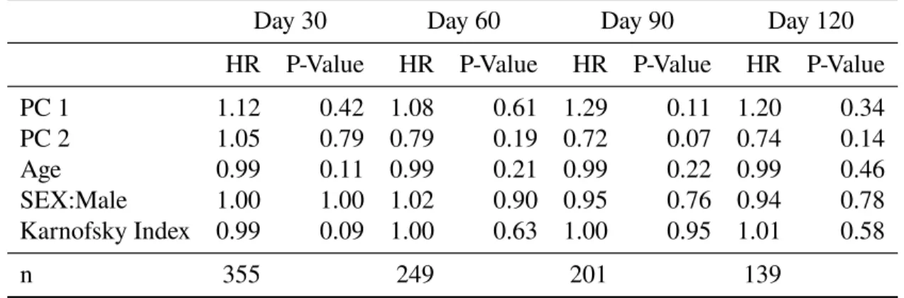
4.5 MPACT trial . . . 59

CHAPTER 5: ROBUST ESTIMATION OF MULTISET CANONICAL COR-RELATION ANALYSIS . . . 67

5.1 Introduction . . . 67

5.2 Multi-set Canonical Correlation Analysis . . . 68

5.3 High dimensional robust mCCA. . . 72

5.3.1 High-dimensional CCA methods. . . 72

5.3.2 Robust correlation estimation in transelliptical family . . . 74

5.3.3 Latent high-dimensional mCCA in the transelliptical family . . . 76

5.3.4 Selecting number of principal directions for each set and identi-fying informative canonical correlation vectors . . . 78

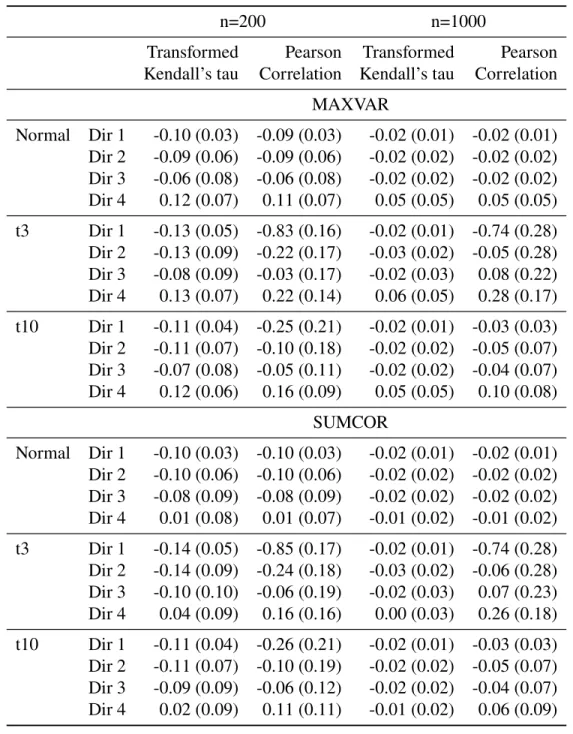
5.4 Simulations Results . . . 83

5.4.1 Estimation of canonical directions . . . 85

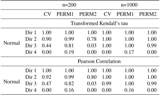
5.4.2 Identifying informative canonical directions . . . 87

5.5 mCCA estimates for executive function and brain structure in six-year-old children . . . 94

CHAPTER 6: SUMMARY AND FUTURE RESEARCH. . . 101

APPENDIX A: TECHNICAL DETAILS AND ADDITIONAL SIMULATION RESULTS FOR CHAPTER 2 . . . 104

A.1 Proof of theorems . . . 104

A.2 Additional Simulation Results . . . 108

(9)

A.2.2 Confidence intervals for canonical correlations and canonical

direction loadings . . . 115

A.2.3 Testing for non-zero canonical correlations . . . 122

A.3 Additional results for White matter tractography data and executive function in six year old children . . . 124

APPENDIX B: TECHNICAL DETAILS AND ADDITIONAL SIMULATION RESULTS FOR CHAPTER 3 . . . 127

B.1 Proof of Theorems . . . 127

B.2 Additional Simulation Results . . . 134

B.2.1 True correlation matrices for martingales and counting processes . . . 134

B.2.2 Additional simulation results . . . 137

B.3 Principal component Loadings for MPACT data. . . 141

APPENDIX C: ADDITIONAL RESULTS FOR CHAPTER 4 . . . 143

C.1 Multi-set Canonical Directions for Executive Function and Brain Struc-ture Data . . . 143

(10)

LIST OF TABLES

3.1 Bias (SD) of canonical correlation and direction estimates, p=q=8, n=200 . . . 26 3.2 Power and type I error for asymptotic, permutation and bootstrap testing procedures 29 3.3 List of white matter tracts used in CCA analysis . . . 30 3.4 Estimates for first canonical correlation and directions for white matter

tract RD values and EF tests for transelliptical and standard CCA . . . 33 3.5 Estimates for first canonical correlation and direction for RD lateralization

measure and EF tests for transformed Kendall’s CCA and standard CCA . . . 35 4.6 Average (SD) of the angle in radians between the true and estimated PCA

directions based on counting process and martingale correlation matrices

with no competing risks . . . 57 4.7 Average (SD) of the angle in radians between the true and estimated PCA

in the presence of a competing risk . . . 58 4.8 Principal component directions at day 360 and proportion of variance

explained for each principal component using estimates based on martingale

covariance matrix . . . 60 4.9 Estimated hazard ratios for landmarked Cox PH models using PC score

estimates as covariates . . . 63 4.10 Comparison of average PC 1 scores and PC 2 scores for patients who

died/progressed before landmark date compared to those who survived up

to landmark date . . . 65 5.11 Bias (SD) of estimated MAXVAR/VAR direction MAXVAR value

com-pared to true direction MAXVAR value and estimated SUMCOR/AVGVAR direction compared to true direction SUMCOR value, selecting between

three and nine principal components per set . . . 88 5.12 Average (SD) of the correlation between estimated and true MAXVAR/VAR

directions and SUMCOR/AVGVAR directions, selecting between three and

nine principal components per set . . . 89 5.13 Type I error for CV and permutation testing procedures using correlation

structure two. . . 91 5.14 Power and type I error for cross-validation and permutation testing

(11)

5.15 Power and type I error for cross-validation testing procedure for correlation

structure one when data come from multivariate t distribution . . . 94

5.16 List of white matter tracts used in CCA analysis . . . 95

5.17 Cross-validated correlation matrices for MAXVAR/VAR mCCA directions . . . 97

A1 Bias (SD) of canonical correlation and direction estimates, p=q=4, n=200 . . . 110

A6 Bootstrap and asymptotic confidence interval coverages for transelliptical canonical correlations, p=q=4 . . . 116

A9 Bootstrap and asymptotic confidence interval coverages for transelliptical canonical directions for data with multivariate normal distribution, p=q=4 . . . 117

A10 Bootstrap and asymptotic confidence interval coverages for transelliptical canonical directions for data with multivariate Cauchy distribution, p=q=4 . . . 118

A12 Bootstrap and asymptotic confidence interval coverages for transelliptical canonical directions for data with multivariate Cauchy distribution, p=q=8 . . . 119

A14 Bootstrap and asymptotic confidence interval coverages for transelliptical canonical directions for data with multivariate Cauchy distribution, p=q=16. . . 121

A15 Power and type I error for permutation and bootstrap testing procedures using standard correlation estimates. . . 123

(12)

A17 Estimates for first canonical correlation and directions for white matter

tract AD values and EF tests for transelliptical and standard CCA . . . 126 B18 Average (SD) of the angle in radians between the true and estimated PCA

with no competing risks . . . 139 B19 Average (SD) of the angle in radians between the true and estimated PCA

in the presence of a competing risk . . . 140 C20 MAXVAR/VAR multi-set canonical correlation analysis direction loadings

for executive function variables . . . 143 C21 MAXVAR/VAR multi-set canonical correlation analysis direction loadings

for diffusion tensor imaging white matter tracts . . . 144 C22 MAXVAR/VAR multi-set canonical correlation analysis direction loadings

for grey matter volume regions . . . 145 C23 MAXVAR/VAR multi-set canonical correlation analysis direction loadings

for grey matter volume regions . . . 146 C24 MAXVAR/VAR multi-set canonical correlation analysis direction loadings

(13)

LIST OF FIGURES

4.1 Principal component direction loadings from day 30 to 360 for first two principal components using martingale correlation matrix estimates. Line

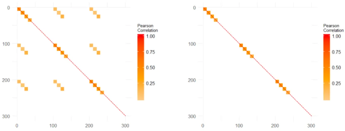
types indicate constitutional, gastrointestinal and hematologic event types. . . 60 5.2 Correlation structure one on the left and correlation structure two on the right . . . 85 5.3 GM and DTI loadings for first canonical direction using MAXVAR/VAR formulation 98 5.4 GM and DTI loadings for second canonical direction using MAXVAR/VAR

formulation . . . 99 B.3.5 Principal component direction loadings from day 30 to 360 for first two

principal components using martingale correlation matrix estimates. Line

(14)

LIST OF ABBREVIATIONS

AD Axial Diffusivity

ARC FP Arcuate fasciculus indirect anterior pathway ARC FT Arcuate fasciculus direct pathway

ARC TP Arcuate fasciculus indirect posterior pathway BASC Behavioral Assessment System for Children BRIEF Behavior Ratinv Inventory of Executive Function CANTAB Cambridge Neuropsychological Test Automated Battery CCA Canonical Correlation Analysis

CGC Anterior cingulum

CIF Cumulative Incidence Function

CTPF Corticothalamic prefrontal projections

CV Cross Validation

DTI Diffusion Tensor Imaging

EF Executve Function

FA Fractal Anisotropy

GM Grey Matter

IFOF Inferior fronto-occipital fasciculus ILF Inferior longitudinal fasciculus

LOESS Locally Estimated Scatterplot Smoothing MCD Minimum Covariance Determinant mCCA Multiset Canonical Correlation Analysis PCA Principal Components Analysis

PH Proportional Hazards RD Radial Diffusivity

(15)

SLF Superior longitudinal fasciculus SOC Stockings of Cambridge

SSP Spatial Span

SVD Singular Value Decomposition

(16)

CHAPTER 1: INTRODUCTION

Many medical or public health data sets have a large number of variables that are collected across the same subjects. Methods such as canonical correlation analysis (CCA) and principal components analysis (PCA) are useful for summarizing entire data sets into a small number of linear combinations of the data. These low dimension representations of the data can make it easier for medical and scientific researchers to understand the structure of complex data sets which can lead to new scientific hypotheses or discoveries.

(17)

Next we consider the multivariate survival setting, where we observe time to event data for many different types of adverse events across the same subjects. The time to event for all of these events may be right censored. In the presence of censoring the covariance between the failure times cannot be estimated without strong parametric assumptions. We instead focus on the counting processes or martingales defined by the failure times. The full covariance or correlation matrices of these counting processes and martingales can be estimated non-parametrically. We use the estimates of the counting process and martingale covariance or correlation matrices to estimate the corresponding principal directions. We also show how this can be extended to the semi-competing risk setting where each of the different event types is subject to a competing risk such as death. We apply our martingale PCA method to data from a clinical trial for patients with pancreatic cancer and are able to define medically relevant groupings of adverse events.

Finally we extend CCA to the multi-set and high-dimensional setting. In this case there are more than two sets of variables, and we use multi-set CCA (mCCA) to get a low dimensional representation of the linear correlation between all the sets of variables. As with standard CCA, previous methods for mCCA work best when data come from a multivariate normal distribution. We combine previously developed methods for mCCA in the high-dimensional setting with our robust correlation techniques to define a robust version of mCCA. We propose a method based on cross-validation for reducing the dimension of the data and identifying informative directions for multi-set CCA. This allows us to include additional brain volume measures across 88 different regions in our analysis of brain imaging and EF data for six-year-old children, and provide added insight for the connection between brain structure and EF ability in children.

(18)

CHAPTER 2: LITERATURE REVIEW

Canonical Correlation Analysis

Canonical Correlation Analysis (CCA) first introduced by Hotelling (1936) is a useful technique for summarizing the linear association between two sets of variables. CCA finds the linear combinations of the two sets of variables that are maximally correlated. Subsequent canonical directions and correlations are found in the same manner subject to the constraint that they are uncorrelated with all previous directions. The solution to the canonical correlations and directions are based on an eigendecomposition involving the joint covariance matrix of the two sets of variables. This is a powerful data reduction technique that allows researchers to look at a much smaller set of correlations than all possible pairwise correlations.

Robust CCA

(19)

estimators is that they primarily focus on data from heavy tailed distributions and do not work well for data from skewed distributions.

Kendall’s tau

One alternative to Pearson’s correlation is Kendall’s tau (Kendall, 1938) which uses the ranks of the data within a sample. For two random variables,X(1)_and_X(2)_{, Kendall’s tau is} defined as

τ(X(1),X(2)) =E[sign(X(1)−X˜(1))(X(2)−X˜(2))],

where [ ˜X(1)_,_X_˜(2)_] is an identically distributed copy of _[_X(1)_{, X}(2)_]. If _[_x(1) 1 , x

(2)

1 ]T, . . . ,

[x(1)n , x(2)n ]T are iid realizations of[X1, X2]T then Kendall’s tau can be consistently estimated by

ˆ

τn(X(1), X(2)) = 1 n

2

X X

1≤k<l≤n

sign(x(1)_k −x(1)_l )sign(x(2)_k −z(2)_l )

Consistency and asymptotically normality follow from U-statistic theoryHoeffding (1961), which makes minimal distributional assumptions on[X(1), X(2)]T.

Elliptical and transelliptical families of distributions

Anyp×1dimensional random vector,Z, is elliptically distributed if it has a characteristic functionΦZ−µ(t) = ψ(tTΣt)whereµis a p-dimensional vector,Σis ap×ppositive

semi-definite matrix and ψ is a function from [0,∞) → _R. This family of distributions includes a number of well known distributions including the multivariate normal and multivariate t distributions. There are a number of theoretical results that can be extended to the entire family of elliptical distributions. One such result is the relationship between the population Kendall’s tau, τ, and Pearson correlation,ρ, for any bivariate elliptical distribution where Pearson correlation exists. Lindskog et al. (2003) shows the following equivalence holds for all such distributions:

τ = 2

(20)

This relationship is also useful for the transelliptical family of distributions, defined by Liu et al. (2012), which includes any multivarate distribution created by transforming an elliptical distribution with a set of univariate monotonic transformations. This is equivalent to the family of multivariate distributions with an elliptical copula (Embrechts et al., 2002; Klüppelberg and Kuhn, 2009). Because Kendall’s tau is invariant to monotone increasing marginal transformations of the data it is very useful for transelliptical distributions. Recent studies have investigated using transformations of Kendall’s tau to estimate the correlation matrix for elliptical and transelliptical distributions (Han and Liu, 2012). This estimator has been shown to work well in high dimensions (Han and Liu, 2013, 2017).

Distribution of canonical correlations and directions

Anderson (2003) shows that CCA estimates corresponding to unique non-zero canonical correlations are asymptotically normal when using the sample covaraince matrix and the data come from multivariate normal distribution. Taskinen et al. (2006) extends this result to elliptical distributions and covariance or correlation estimates that are positive definite functions of the data.

High dimensional Canonical Correlation Analysis

For many modern data sets the number of variables can be larger than the number of observations. Standard CCA estimation techniques do not work in this setting. A number of methods have been proposed for this purpose. One approach for high dimensional CCA is to add a penalty term to the canonical directions (Suo et al., 2017; Witten et al., 2009; Parkhomenko et al., 2007; Waaijenborg et al., 2008; Wilms and Croux, 2016). Vinod (1976) proposes applying a ridge penalty directly to the estimates of the covariance matrix, which can then be decomposed to get the CCA estimates.

Multiset Canonical Correlation Analysis

(21)

(1971) give an overview of the different ways to extend CCA into multiple sets of variables. In this case we havemsets of variables,X1, . . . , Xm, whereXiis andi×1random vector. For

theithset of variables we can define thejthcanonical variate asU_i(j) =a(_ij)TXi. Kettenring

(1971) presents five different ways to think of maximizing the correlation between the canonical variates

1. SUMCOR: Maximize

m

P

i=1

m

P

k=1

Cov(U_i(j), U_k(j))

2. MAXVAR: Maximize the largest eigenvalue for the covariance matrix of[U₁(j), . . . , Um(j)]T

3. MINVAR: Minimize the smallest eigenvalue for the covariance matrix of[U₁(j), . . . , Um(j)]T

4. SSQCOR: Maximize

m

P

i=1

m

P

k=1

Cov(U_i(j), U_k(j))2

5. GENVAR: Minimize the determinant of the covariance matrix of[U₁(j), . . . , Um(j)]T

Nielsen (2002) extended this by allowing for four different constraints on the direction vectors, a(_ij).

1. NORM:a(_ij)Ta_i(j) = 1fori= 1, . . . , d.

2. AVGNORM:Pd

i=1a (j)T

i a

(j)

i = 1

3. VAR: Var(U₁(j)) =. . .=Var(U_d(j)) = 1.

4. AVGVAR:Pd

i=1Var(U (j)

i ) = 1.

This allows for 20 different formulations of the multiset CCA problem. Asendorf (2015) gives a useful overview of the 20 different formulations and shows which have closed form solutions. Principal Components Analysis

(22)

variables that explain the maximum variance subject to the constraint that they are uncorrelated with all previous directions. The principal directions can be shown to be the eigenvectors of the joint covariance matrix of the variables. Estimates of the principal directions are typically the eigenvectors of the sample covariance matrix of the observed data. PCA can be used for both dimension reduction and reducing multicollinearity between the variables. Frequently a large proportion of the variance within a set of variables can be explained by a small number of principal components. Collinearity among predictors can create instability in estimation for various statistical methods including linear regression. Principal component regression deals with this issue by including the uncorrelated principal component scores instead of the original data. Anderson (2003) shows that if the data come from a multivariate normal distribution the estimation of the eigenvalues and eigenvectors of the sample covariance matrix are asymptotically normal when properly standardized.

Estimates of bivariate survival function

Bivariate or multivariate survival data can come in the context of paired or clustered subjects all with a single survival time, or a single person with multiple non-competing failure times. In the bivariate case theithsubject or cluster will have two failure timesT(1) and_T(2) as well as two censoring timesC(1)andC(2). The bivariate survival function for the failure times is

S(1,2)(t, s) =P(T(1) > t, T(2) > s).

If we define X(j) = min(T(j), C(1)) and δ(j) = I(X(j) = C(j)), the observed data will be

(23)

Survival Analysis with Semi-Competing Risks

In many settings failure times can be subject to both independent censoring and competing risks. This includes time to event data for certain diseases in which death acts as a competing risk. This means that once death is observed the disease of interest will never be observed. This competing risk set up can extend both the univariate and bivariate survival set up. In the bivariate competing risk set up there are still two failure times of interest, T₁(1) and T₁(2). In addition, for each failure time of interest there is also a competing risk time, T₂(1) and T₂(2). Without censoring the observed data isT(j) = T₁(j)∧T₂(j) and(j) = 2−I(T₂(j) > T₁(j))for

j = 1,2. If we introduce an independent censoring time for each failure time of interest,C(1) andC(2)_{, the observed data will be}_X(j)₌_T(j)_∧_C(j)_,_δ(j)₌_I₍_T(j) _≤_C(j)₎_{, and}_η(j)₌_δ(j)(j) forj = 1,2. For this competing risk set up it has been shown that the cause specific cumulative

incidence functions (CIF) can be estimated non-parametrically. The univariate cause specific CIF isF_k(j)(tj) =P(T(j) ≤tj,¨(j) =k)forj = 1,2andk = 1,2. Details on estimation of the

univariate cause specific CIF can be found in Kalbfleisch and Prentice (2011). The bivariate cause specific CIF is defined asF_kl(j,j0)(tj, tj0) = P( ¨T(j) ≤t_j,γ¨(j) =k,T¨(j

0₎

≤ tj0,γ¨(j 0₎

=l),

forj, j0 = 1,2andk, l= 1,2. Details on estimation of the bivariate cause specific CIF can be

found in Cheng et al. (2007). Functional delta method

The delta method is a well known result that can be used to derive the distribution of functions of random variables. When an estimator is a functional the functional delta method (Kosorok, 2008) can be used for the same purpose. In order to give the functional delta method we must first define the concept of Hadamard differentiability. For two complete normed spaces

DandEa mapφ : D → Eis Hadamard differentiable athif there exists a mapφ0θ : D→ E

such that

φ(θ+tnhn)−φ(θ)

tn →φ

0

(24)

then φ is Hadamard differentiable with derivative φ0_θ. With this definition we can give the functional delta method which is theorem 2.8 from Kosorok (2008).

Functional delta method For normed spacesDandE, letφ : Dφ ⊂ D → Ebe Hadamard

differentiable atθtangentially toD0 ⊂D. Assume thatrn(Xn−θ) X for some sequence of

constantsrn → ∞, whereXntakes it’s values inDφandX is a tight process taking it’s values

(25)

CHAPTER 3: CANONICAL CORRELATION ANALYSIS FOR ELLIPTICAL COPU-LAS

3.1 Introduction

Canonical correlation analysis (CCA), first introduced by Hotelling (1936), is a useful dimension reduction technique for exploring the relationship between two sets of variables. CCA finds the linear combinations of the two sets of variables that have maximal Pearson correlation. After the first direction, further directions are defined as the linear combinations that are maximally correlated subject to the constraint that they are uncorrelated with all previous directions. Typically a small number of directions may be used to summarize the relationship between the two sets of variables.

In Section 3.4 we present an example where CCA is useful in understanding the relationship between the structure of white matter brain tracts and executive function in six-year-old children. Many of the variables have excess skewness or kurtosis relative to the normal distribution. This suggests transformations may be needed for CCA using Pearson’s correlation to fully capture the association between the two sets of variables. However it is not clear how to optimally transform the data, especially for heavy tailed distributions where transforming may weaken linear associations. In such settings, standard CCA may be problematic, and alternative approaches are valuable.

(26)

rich literature on robust estimators of the covariance matrix that are insensitive to outliers and heavy tailed distributions, and may improve the performance of standard CCA based on Pearson correlation. Examples of these are the minimum covariance determinant (MCD) (Rousseeuw, 1984) and Tyler’s (1987) M-estimator. There have been studies examining the performance of CCA using robust estimators of the covariance matrix or by maximizing other robust correlation measures (Taskinen et al., 2006; Visuri et al., 2003; Branco et al., 2005; Alfons et al., 2017). Many of these robust methods emphasize eigendecompositions employing robust estimates of the covariance or Pearson correlation matrix, which do not exist in the absence of finite moments. Further assumptions are needed to interpret robust CCA in these settings.

(27)

distribution by estimating the scatter matrix based on transformations of Kendall’s tau for all pairs of variables (Liu et al., 2012). We establish that the resulting estimates for CCA directions and non-zero correlations are consistent and asymptotically normal. This result is more general than previous results which require affine equivariant estimators of the scatter matrix for elliptically distributed data (Anderson, 1999; Taskinen et al., 2006). Interestingly, the estimate based on transformations of Kendall’s tau for all pairs of variables is not affine equivariant. Simulations show that these results can be used to construct confidence intervals with close to the desired coverage.

We also develop a testing procedure to identify non-zero canonical correlations using boot-strap bias and standard error estimates. This is necessary because although the asymptotic results for non-zero canonical correlations can be used to construct confidence intervals, asymptotic results for zero canonical correlations are not as straightforward. However based on previous results (Anderson, 2003) it can be expected that the zero canonical correlations will converge at ratenrather than√n. Therefore by inverting a normal bootstrap confidence interval we derive a test that is consistent and conservative for large sample sizes. This testing procedure can be used for CCA estimated using Kendall’s tau or standard methods. This testing procedure is necessary because previously derived asymptotic tests assume the data come from a multivariate normal distribution. Even permutation based tests assume that zero correlation implies independence, which is not true for non-Gaussian elliptical copulas. Both of these types of tests will have inflated type I error when their assumptions are not met. Our bootstrap based testing procedure makes no such assumptions, and is useful even when data do not have an elliptical copula.

(28)

3.2 Rank correlation methodology

AssumeX is ap×1dimensional random vector andY is aq×1dimensional random

vector. The first canonical directions forXandY are thep×1vector,a1, and theq×1vector,b1, for which the correlation betweenU1 =aT1XandV1 =bT1Y is maximized. The first canonical correlation is defined as the Pearson’s correlation betweenU1andV1. In order to uniquely define a1 andb1, it is necessary to add the constraints that Var(U1) = Var(V1) = 1(Hotelling, 1936). After the first canonical direction and correlation, higher directions are a sequence of p×1

vectors,aj, andq×1vectors,bj, such thatUj =aTjXandVj =bTjY are maximally correlated,

subject to the constraints that cor(Uj, Uj0) = cor(U_j, V_j0) =cor(V_j, U_j0) =cor(V_j, V_j0) = 0for allj0 < j, and Var(Uj) =Var(V1) = 1for allj. This uniquely defines the canonical directions corresponding to a non-zero canonical correlation except for multiplication of bothaiandbiby

−1. There are at mostmin(p, q)non-zero canonical correlations assuming bothXandY are full rank.

The canonical directions and correlations forX andY can be shown to be the solutions to an eigendecomposition based on the covariance matrix betweenXandY. Estimates of the canonical directions and correlations are commonly based on the same eigendecomposition of the sample covariance matrix. If we define the joint covariance matrix ofXandY as

Cov([XT, YT]T) =



 

ΣXX ΣXY

ΣY X ΣY Y



 

then the canonical correlations and directions may be derived from:

C = Σ−_XX1/2ΣXYΣ−Y Y1 ΣY XΣ

−1/2

XX , and

D= Σ−_{Y Y}1/2ΣY XΣ−XX1 ΣXYΣ

−1/2

(29)

The matricesCandDshare the same firstmin(p, q)eigenvalues, which are the square root of

the canonical correlations. Ifvciis theitheigenvector ofC, thenvciΣ

−1/2

XX =ai, and ifvdiis the

itheigenvector ofD, thenvdiΣ

−1/2

Y Y =bi.

CCA can be made robust via robust estimation of the covariance matrix. Many robust estimates of the covariance matrix are consistent under the elliptical family of distributions, defined as,

Definition 3.1( Elliptical Distributions). Ad×1random vectorZ is considered to be elliptical if for some d ×1 vector µZ, some d ×d positive semi-definite matrix ΣZ, and a function

ψZ[0,∞) → R, the characteristic function, Φ, satisfiesΦZ−µZ(t) = ψ(t

T_Σ

Zt)for alld×1

vectorst. In this case we would say thatZis ad×1dimensional elliptically distributed random variable, which we can note asZ ∼EDd(µZ,ΣZ, ψZ)

We useΣZ in definition 3.1 because in the elliptical distributionΣZ can be viewed as a

generalization of the covariance matrix for Z. When second moments exist ΣZ equals the

covariance matrix up to a scaling factor, and ψZ can be chosen such that it is equal to the

covariance matrix. We will refer toΣZas the scatter matrix ofZ, which exists even if second

moments do not exist. The following proposition shows that for linear combinations of Z, the scatter matrix,ΣZ behaves in the same way as a covariance matrix. To be precise, linear

combinations of elliptical random variables are also elliptically distributed with a scatter matrix which is a quadratic form inΣZ.

Proposition 3.1(Linear combinations of elliptically distributed random variables). Assume Z ∼EDd(µZ,ΣZ, ψZ). DefineB to be ak×ddimensional matrix. ThenW =BZ is ak×1

dimensional random vector whereW ∼EDk(BµZ, BΣZBT, ψW)

(30)

LettingZ = [XT_{, Y}T_]T_{, the scatter matrix of}_Z_{can be decomposed as}

ΣZ =



 

ΣXX ΣXY

ΣY X ΣY Y



 .

Next we introduce the concept of the scale-invariant scatter matrix ofZ, PZ, which will be

equivalent to the correlation matrix ofZ when second moments exist. Analogously toΣZ,PZ

may be written as,

PZ =



 

PXX PXY

PY X PY Y



 .

The elements ofPZ,ρij, are related to the elements ofΣZ,σij, through the following equality,

ρij = σij

√

σii√σjj. In generalΣZandPZwill be assumed to be positive-definite in order to guarantee existence of unique solutions for canonical correlation analysis.

A useful extension of elliptical distributions is the transelliptical family of distributions, whose definition is given below,

Definition 3.2 (Transelliptical distributions). Ad ×1dimensional random vector Z has a transelliptical distribution if there exists a positive-semidefinite matrixPZ with all ones along the

diagonal, a functionψZ : [0,∞)→R, and a set of functionshZ1, . . . , hZdwherehZi:R→R

is a monotone increasing function for i = 1,2, . . . , d such that [hZ1(Z1), . . . , hZd(Zd)]T ∼

EDd(0, PZ, ψZ). The random variableZ is ad×1dimensional transelliptically distributed

random variable, denoted asZ ∼T Ed(hZ,0, PZ, ψZ).

The elliptical distribution used in Definition 3.2 is scale invariant and has a scatter matrix with all ones along the diagonal as well as centrality parameter zero in order to uniquely identify the transformations, hZ. This definition was given by Liu et al. (2012), but an equivalent

(31)

For the elliptical and transelliptical distributions we propose an alternative definition of CCA using a rank correlation measure. This version of CCA is equivalent to standard CCA based on Pearson correlation in the elliptical family when second moments exist and still well defined if they do not exist. This construction uses properties of the rank correlation measure, Kendall’s tau. For two univariate random variablesZiandZj with joint CDFF(Zi, Zj)Kendall’s tau is

τ(Zi,Zj)₌_E{sign₍_Z

i−Z˜i)(Zj −Z˜j)}

where[ ˜Zi,Z˜j]T is an identically distributed copy of[Zi, Zj]T. This quantity exists for all bivariate

continuous distributions, and does not require the existence of moments. A consistent estimator of Kendall’s tau based on n iid copies ofZi andZj,[zi1, zj1]T, . . . ,[zin, zjn]T, is

ˆ

τ(Zi,Zj)

n =

1 n

2

X X

1≤k<l≤n

sign(zik−zil)sign(zjk−zjl)

This estimator is a U-statistic with consistency and asymptotic normality coming from established U-statistic theory (Hoeffding, 1961).

Within the transelliptical family the following property gives the correspondence between Kendall’s tau and the elements of the transelliptical scatter matrix.

Proposition 3.2(Kendall’s tau for transelliptically distributed random variables). AssumeZ ∼ T Ed(h,0, PZ, ψZ). Ifpijis thei−jthentry ofPZandτ(Zi,Zj)is the Kendall correlation between

theithandjthentries ofZ thenτ(Zi,Zj) ₌ 2

π arcsin(ρij)

(32)

Kendall’s tau to zero. Importantly this relationship still holds between elements of the scale invariant scatter matrix and Kendall’s tau for transelliptical distributions when moments do not exist.

Given propositions 3.2 and 3.1 we define CCA for transelliptically distributed data as follows, Definition 3.3( Canonical correlation analysis for transelliptical distributions). AssumeX is ap×1dimensional random vector andY is aq×1dimensional random vector, and that the random vector[XT, YT]T = Z ∼ T Ep+q(hZ,0, PZ, ψZ). DefinehX to be the element-wise

functions ofhZcorresponding toXandhY to be the element-wise functions ofhZcorresponding

toY. The first canonical direction vectors, thep×1vector, a1, and theq×1vector,b1, are the vectors that maximizeτ(U1,V1) _where_U

1 = aT1hX(X)and V1 = bT1hY(Y), subject to the

constraint thatU1andV1have scale parameter equal to one. Thejthcanonical direction vectors are thep×1vectoraj and theq×1vectorbj that maximizeτ(Uj,Vj) whereUj = aTjhX(X)

Vj =bTjhY(Y), subject to the constraints thatτ(Uj,Uj0) =τ(Uj,Vj0)=τ(Vj,Uj0)=τ(Vj,Vj0)= 0for

allj0 < j, and the scale parameter forUj andVj are equal to one for allj. Thejthcanonical

correlation can be defined assin π₂τ(Uj,Vj)_.

When second moments exist and[XT_{, Y}T_]T has an elliptical distribution this definition

is equivalent to performing CCA based on the correlation matrix. When data are elliptically distributed but moments do not exist CCA for the transelliptical family uses the same eigende-composition of the scatter matrix as standard CCA. A large advantage of this is definition is when[XT_{, Y}T_]T _{is transelliptically, but not elliptically distributed. In this setting standard CCA}

depends heavily on the marginal distributions of the variables inXandY, which depends onhX

andhY. In many caseshX andhY can act to obscure potential linear relationships between the

variables. Definition 3.3 is based onPZ, which does not depend on the marginal distributions

of the data. In this sense CCA using Definition 3.3 can be thought of as first transforming the variables to elliptical symmetry and then performing CCA. As shown in proposition3.1linear

(33)

An issue with estimating CCA for the transelliptical family is estimation of a scatter matrix of transformed versions ofXandY. If[XT_{, Y}T_]T ₌_Z _{is transelliptically distributed and}_h

X,

hY, andψZ are all unknown, then all three must be estimated to transformZto it’s underlying

elliptical distribution. Many methods assume thatψZis the generating function from a Gaussian

distribution, which can introduce bias if this assumption is not met. In order to avoid estimation ofhX,hY andψZ we directly estimate the scatter matrix in the transelliptical distribution as

follows (Liu et al., 2012),

Definition 3.4( Transelliptical scatter matrix estimate). Assume thatZ ∼T Ed(hZ,0, PZ, ψZ).

Assume thatρij is the element ofPZ corresponding to theithandjthelements ofZ. Then we

can estimateρij asρˆn,ij = sin

n

π

2τˆ (Zi,Zj)

n

o

,andPZby estimating all individual entries in this

manner. We will refer to this estimator of the scatter matrix,PˆZn, as the transformed Kendall’s

scatter matrix estimator.

To obtain estimates for the canonical directions and correlations for the transelliptical family, we simply decompose the transformed Kendall’s scatter matrix estimator as we would any correlation matrix estimate when conducting CCA. We note that the transformed Kendall’s scatter matrix estimator is the only known estimate of the scatter matrix that can be used for CCA for all members of the transelliptical family, without having to estimate the transformations hZ, or the generatorψZ.

There are other rank based methods that can be used to estimate the scatter matrix for transellipticals whenψZ is assumed to be the generating function for the Guassian distribution.

(34)

distributed and the generating function,ψZ, is from an elliptical distribution other than a Guassian

this method results in biased estimates of the transelliptical scatter matrix.

A potential issue with the transformed Kendall’s scatter matrix estimator is that it is not guaranteed to be positive-definite even when the true scatter matrix, PZ, is positive-definite.

As discussed by Rousseeuw and Molenberghs (1993) various methods are available to adjust

ˆ

PZn so that it is positive-definite. For simplicity we defineP˜Znto be the matrix with the same

positive eigenvalues as_Pˆ_Zn _{but with with all negative eigenvalues set set to some small positive}

constant._P˜_Zn_{will have the same asymptotic behavior as}_Pˆ_Zn_{based on the following theorem:}

Theorem 3.1(Transformed Kendall’s scatter matrix estimator eigenvalues). Assumez1, . . . , zn

ared-dimensional iid realizations of transelliptically distributed vector,Z, with positive-definite scale invariant scatter matrixPZ. Define the ordered eigenvalues of the transformed Kendall’s

scatter matrix, PˆZn to beλˆn1, . . . ,λˆnd, where ˆλnd is the minimum eigenvalue of PˆZn. Then

P r(ˆλnd >0)→p 1

A proof of theorem 3.1 is presented in Appendix A. Theorem 3.1 gives that the probability of _P˜

Zn being equal toPˆZn converges to one for transelliptically distributedZ with

positive-definite PZ. This means for transelliptical Z when PZ is positive-definite

√

n( ˜PZn − PZ)

and √n( ˆPZn − PZ) will have the same limiting distribution. The limiting distribution of

√

n( ˆPZn−PZ)can be shown to be asymptotically normal with mean zero and finite variance

based on U-statistic theory and the delta method. Theorem 3.2 establishes conditions under which the estimates of transelliptical CCA directions and correlations will be consistent and asymptotically normal.

Theorem 3.2(Asymptotic results for transelliptical CCA). Assume[xT

i, yiT]T fori= 1, . . . , n

are iid realizations of the (p + q) × 1 dimensional random vector [XT_{, Y}T_]T ₌ _Z _∼

T Ep+q(hZ,0, PZ, ψZ), with positive-definite PZ. Further assume that p ≥ q and there are

r ≤ q unique non-zero transelliptical canonical correlations for X and Y. Let λ1, . . . , λr

(35)

Λr = diag(λ1, . . . , λr) to be the diagonal matrix with the ordered non-zero canonical

cor-relations on the diagonal. LetAr= [a1, . . . , ar]be thep×rmatrix where theithcolumn is the

ithtranselliptical canonical direction forX, andBr = [b1, . . . , bTr]be theq×rmatrix where

theithcolumn is theithtranselliptical canonical direction forY. DefineAr+ = [a_r₊₁, . . . , a_p] andBr+ = [a_r₊₁, . . . , b_q]to be a solution to the canonical directions corresponding to the zero canonical correlations. This means forA = [Ar, Ar+]and B = [B_r, B_r+], ATP_XXA = I_p,

BT_P

XXB = Iq, andATPXYB =



 

Λq 0

0 0





.Note thatAr and Br are well defined up to a sign change andAr+ andB_r+ are well defined up to multiplication by an orthogonal matrix on the right. Ar+ andB_r+ can be made unique by imposing suitable constraints. We will assume that the estimates ofΛr,Ar andBr, which we will denote asΛ∗nr,A

∗

nr, andB

∗

nr are based on

the eigendecomposition of a function of a consistent estimate of the scatter matrix,PZ, which is

denoted byP_Zn∗ . For an arbitrary matrix,M, define vec(M)to be the column vector made by stacking the columns ofM on top of each other. The following holds: ifP_Zn∗ is guaranteed to be positive-definite and

√ n



    

vec(P_XXn∗ )

vec(P_{XY n}∗ )

vec(P_{Y Y n}∗ )

−

vec(PXX)

vec(PXY)

vec(PY Y)



    

→d Np3_×_q3(0,Θ),

then √n[vec(Λ∗_nr)−vec(Λr)],√n[vec(A∗_nr)−vec(Ar)]and √n[vec(B∗_nr)−vec(Br)]jointly have multivariate normal limiting distributions with mean zero and a finite limiting variance that is a function ofΘ,A,B, andΛq. The form of the limiting variance can be found in Appendix A.

(36)

is used. Taskinen et al. (2006) expanded this result to CCA in the elliptical distribution when using positive-definite and affine equivariant estimators of the covariance matrix. Because we make minimal assumptions about the form ofΘwe do not get a concise form of the limiting

variances as in previous results. Because_P˜_Zn_{is not affine equivariant our more general result is}

needed. To our knowledge there are no other estimators of the scatter matrix that work for all transelliptical distributions that do not require the estimation ofhZ andψZ.

We have already shown that_P˜_Zn_{is positive-definite, consistent, and asymptotically normal,}

which leads directly to corollary 3.1.

Corollary 3.1(Asymptotic results for transformed Kendall’s scatter matrix estimator). Assume the same set up as in Theorem 3.2 and thatPZis estimated usingP˜Zn. DefineΛñr,Añr, andBñr

as the corresponding estimates for the non-zero transelliptical canonical correlations and their corresponding transelliptical canonical directions. Then√n[vec( ˜Λnr)−vec(Λ)],

√

n[vec( ˜Anr)−

vec(A)], and√n[vec( ˜Bnr)−vec(B)]jointly multivariate normal limiting distributions with

mean 0 and finite variances. The form of the variances can be found using methods from the proof for Theorem 3.2 in Appendix A.

Methods from Rublík (2016) can be used to obtain estimators for the covariance matrix for all pairwise estimates of Kendall’s tau. An estimate of the variance of_P˜

Zn can then be found

using the delta method, which allows for estimates of the limiting variances for_Λn˜ _,_A˜_n_{, and}_B˜_n

to be estimated by a "plug-in" estimator using the form of the variance found in Appendix A. Section 3.3 and Appendix A include simulations studies that compare the coverage of confidence intervals using this method to bootstrapped confidence intervals.

(37)

It is important to note that Theorem 3.2 and Corollary 3.1 only apply to non-zero canonical correlations and cannot be used for hypothesis testing for zero correlations. Anderson (2003) gives the asymptotic distribution for the zero canonical correlations for standard CCA whenX andY are jointly multivariate normal and show that in this case the estimates of the correlations converge at rate n. In addition Muirhead and Waternaux (1980) shows how test statistics used to test for a true canonical correlation of zero whenX andY are multivariate normal can be modified for elliptical distributions. These results exploit special properties of the elliptical distribution and sample covariance matrix, but it is unclear how to generalize these results to transelliptical CCA using the transformed Kendall’s scatter matrix estimator. Because of this we propose a testing procedure based on bootstrapped replicates. To control the type I error atαsimply invert a (1-2α) bootstrapped confidence interval using the normal approximation with bias correction. A (1-2α) is used because this test is only one sided, so using a(1−α)

interval will unnecessarily reduce power. Other bootstrap confidence intervals may be used, although it is important not to use the simple percentile method. This is because as sample size and dimension increase the probability that for each bootstrap sample the estimated canonical correlation will be above zero converges to one. This means some type of bias correction is necessary. Although the asymptotic distribution for true correlations of zero is not normal, the fact that the correlations converge at ratenas opposed to√nimplies that this bootstrap will have conservative type I error as sample size increases. This is shown in simulation results found in Section 3.3.

(38)

permutation test will lead to inflated type I error if the data do not have a Gaussian copula, and asymptotic testing procedures assume the data come from a multivariate Gaussian distribution. Importantly this means that even if all the marginal distributions are Gaussian, permutation and asymptotic tests will result in inflated type I error if the copula defining the joint distribution is not a Gaussian copula. For this reason we recommend using the inverted bootstrap procedure if there is any reason to believe data do not follow a multivariate normal distribution. The inverted bootstrap procedure does not even need the transelliptical assumption, just the assumption that the estimated correlation or covariance matrix is asymptotically normal. For the transformed Kendall’s estimator this only requires that the data from different subjects be independent and identically distributed, and for the sample correlation or covariance matrix this only requires that the data be independent and identically distributed and fourth moments exist. When using the transformed Kendall’s estimator this bootstrap procedure will test the null that for all variables inXthe true pairwise Kendall’s tau coefficient with all variables inY is 0. Therefore even when data do not have an elliptical copula this provides a meaningful test for association between the two sets of variables. Simulation results comparing the bootstrap testing procedures with other testing procedures are presented in section 3.3.3.

3.3 Simulation Results

3.3.1 Empirical bias and variance of CCA with robust covariance estimation

Simulations are conducted to compare transelliptical CCA using the transformed Kendall’s estimator and standard CCA under both elliptical and transelliptical settings. In addition CCA based on two robust covariance matrix estimators are considered, the minimum covariance determinant (MCD) estimator from the R packagerobustbase(Todorov and Filzmoser, 2009a) and the M estimator from the R packagerrcov(Todorov and Filzmoser, 2009b). Standard CCA is calculated using the R packageCCA.

(39)

but not elliptical family. The sample size of the simulated data sets are n=200 and n=1,000, and the dimension ofX and Y are p=q=4,8 and 16. Results for p=q=8 and n=200 are presented below, with the other results given in Appendix A. The true scatter matrix for X and Y is

ΣXX = ΣY Y = Ip, and ΣXY = diag(0.9,0.5,0.4,1/3,0, . . .). The structure of these scatter

matrices is similar to those in Branco et al. (2005). To define_P˜

Zn all negative eigenvalues are

set to 0.001. For each simulation setting, at most0.2%of simulations resulted inPˆZn not being

positive-definite. The total number of simulated data sets for each simulation setting is 1,000. Based on the 1,000 simulated data sets the empirical bias and standard deviation is calculated for the canonical correlations and directions for each of CCA methods. For the canonical correlation estimates the bias and variance are calculated after a Fisher inverse hyperbolic tangent transformation. For theithcanonical direction the angle between the true direction forX,ai, and

estimated direction forX for thejthsimulation,ˆaji, is calculated ascos−1

_|_a_ˆT ji,ai|

||ˆaT

ji,ˆaji||·||aTi,ai||

. The bias for the canonical directions is estimated as the average angle across all simulated data sets and the standard deviation is estimated as the empirical standard deviation of the angles across all simulated data sets. Table 3.1 gives the output for the canonical correlation and canonical direction. BecauseΣXY is symmetric andp=qonly the bias and standard deviation

for theX direction are presented, with the results forY being nearly identical.

(40)

multivariate t with ten degrees of freedom standard CCA using the sample covariance matrix and the transformed Kendall’s scatter estimator, both of them outperforming the other two methods.. Under the lognormal setting the standard estimator, the MCD estimator, and the M estimator all underestimate the transelliptical canonical correlations, while the transformed Kendall estimator provides consistent estimates. This is particularly evident for n = 1,000

presented in Appendix A. These findings illustrate the advantages of the transelliptical CCA with data that are transelliptically but not elliptically distributed. Even without transforming potentially skewed marginal distributions the transformed Kendall’s scatter estimator can consistently estimate the strongest linear relationships based on the underlying copula. As noted previously, the finite sample bias is positive for both standard and transelliptical canonical correlation estimates.

3.3.2 Confidence intervals for non-zero canonical correlations

Simulations are run to compare coverages for normal bootstrapped confidence intervals as well as asymptotic confidence intervals using "plug-in" estimators of the asymptotic variance for the estimates from Theorem 3.2. Details on the form of the variance estimates are in Appendix A. The "plug-in" variance estimator is calculated using estimates of transelliptical canonical correlations, and directions based on the transformed Kendall’s correlation estimate. An estimate of the variance of the transformed Kendall’s scatter matrix is obtained using methods from Rublík (2016). For the bootstrap confidence intervals 1,000 bootstrap replicates are used. The bootstrap confidence intervals for the canonical correlations are constructed from the square of the estimated canonical correlations, and then transformed using the square root to give the bounds for the transelliptical canonical correlations. Bounds may be truncated at one or zero as necessary for both the bootstrap and asymptotic confidence intervals.

(41)

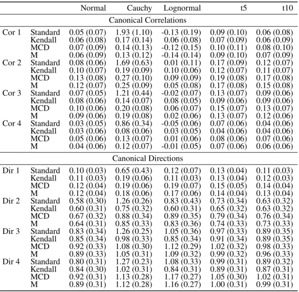
Table 3.1: Bias (SD) of canonical correlation and direction estimates, p=q=8, n=200

Normal Cauchy Lognormal t5 t10

Canonical Correlations

Cor 1 Standard 0.05 (0.07) 1.93 (1.10) -0.13 (0.19) 0.09 (0.10) 0.06 (0.08) Kendall 0.06 (0.08) 0.17 (0.14) 0.06 (0.08) 0.07 (0.09) 0.06 (0.09) MCD 0.07 (0.09) 0.14 (0.13) -0.12 (0.15) 0.10 (0.11) 0.08 (0.10) M 0.06 (0.09) 0.13 (0.12) -0.14 (0.14) 0.09 (0.10) 0.07 (0.09) Cor 2 Standard 0.08 (0.06) 1.69 (0.63) 0.01 (0.11) 0.17 (0.09) 0.12 (0.07) Kendall 0.10 (0.07) 0.19 (0.09) 0.10 (0.06) 0.12 (0.07) 0.11 (0.07) MCD 0.13 (0.08) 0.27 (0.10) 0.09 (0.09) 0.19 (0.08) 0.17 (0.08) M 0.12 (0.07) 0.25 (0.09) 0.05 (0.08) 0.17 (0.08) 0.15 (0.08) Cor 3 Standard 0.07 (0.05) 1.21 (0.44) -0.02 (0.07) 0.13 (0.07) 0.09 (0.06) Kendall 0.08 (0.06) 0.14 (0.07) 0.08 (0.05) 0.09 (0.06) 0.09 (0.06) MCD 0.10 (0.06) 0.20 (0.08) 0.06 (0.07) 0.15 (0.07) 0.13 (0.07) M 0.09 (0.06) 0.19 (0.08) 0.02 (0.06) 0.13 (0.07) 0.12 (0.06) Cor 4 Standard 0.03 (0.05) 0.86 (0.34) -0.05 (0.06) 0.07 (0.06) 0.04 (0.06) Kendall 0.03 (0.06) 0.08 (0.06) 0.03 (0.05) 0.04 (0.06) 0.04 (0.06) MCD 0.05 (0.06) 0.13 (0.07) 0.01 (0.06) 0.08 (0.06) 0.07 (0.06) M 0.04 (0.06) 0.12 (0.07) -0.01 (0.05) 0.07 (0.06) 0.06 (0.06)

Canonical Directions

(42)

asymptotic and bootstrap confidence intervals tend show undercoverage when n=200. This is particularly the case for asymptotic confidence intervals as dimension increases, likely due to the lack of bias correction. Coverage for both the asymptotic and bootstrap confidence intervals improves as sample size increases.

For the transelliptical canonical directions bootstrap and asymptotic confidence intervals are calculated for the loading of each variable in directions corresponding to non-zero canonical correlations. For each bootstrap replicate the estimates of both transelliptical canonical directions are flipped if necessary in order to minimize the sum of the angles between the estimated direction within the bootstrap replicate and the original sample. The coverages are close to95%for the

first canonical direction, with overcoverage for the variable with a non-zero loading for the first direction. For both the bootstrap confidence intervals and asymptotic confidence intervals there is undercoverage for some loadings in the second, third, and fourth directions. This is likely due to the added complexity of additional constraints for higher order canonical directions. We recommend interpreting any confidence intervals for higher order directions with caution. In finite samples it is difficult to fully quantify the uncertainty that arises as the number of constraints increases.

3.3.3 Testing procedures to identify non-zero canonical correlations

In addition to constructing confidence intervals for the non-zero canonical correlations and the associated directions, testing the null hypothesis that the true canonical correlation equals zero is also of interest. As noted in Section 3.2 we propose testing for a true canonical correlation of zero at the0.05significance level by inverting a90%normal bootstrap confidence interval for

the transelliptical canonical correlation, and rejecting the null hypothesis if the lower bound for the confidence interval is above zero. We use a90%confidence interval because the alternative

(43)

moving on to higher order correlations, stopping when the test fails to reject the null hypothesis of a true correlation of zero.

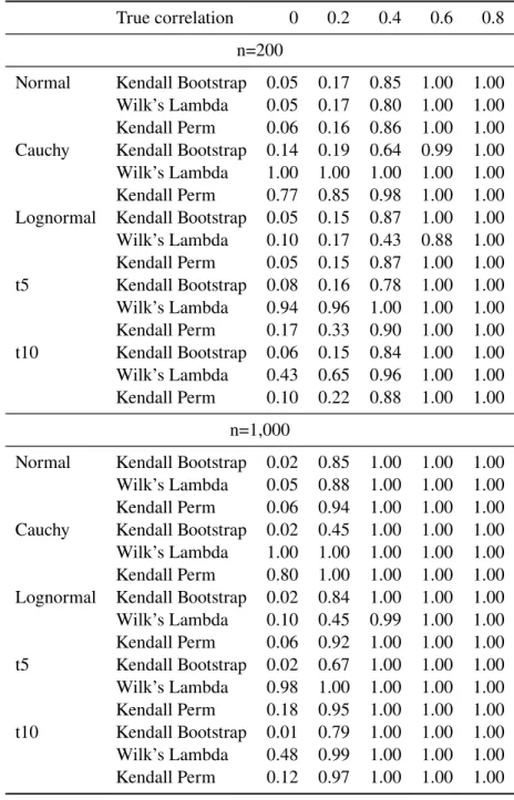
We compare the type I error and power for the bootstrapped testing procedure using the transformed Kendall’s estimator with a permutation test also using the transformed Kendall’s estimator and the asymptotic Wilk’s Lambda from the R packageCCP(Menzel, 2009) using standard CCA based on the sample correlation matrix. In addition the bootstrap and permutation testing procedures using the sample correlation matrix estimator are presented in Appendix A. We consider p = q = 8 and ΣXX = ΣY Y = I where ΣXY has either all zeros or a

single non-zero entry ranging from 0.2 to 0.8 in increments of 0.2. This set up is employed for multivariate normal, multivariate Cauchy, multivariate t with five and ten degrees of freedom, and multivariate lognormal distributions for bothn = 200andn= 1,000. 1,000 data sets are

(44)

distributions also affect this testing procedure. Power for the bootstrap method is generally comparable to the other testing methods, particularly as sample size increases.

Table 3.2: Power and type I error for asymptotic, permutation and bootstrap testing procedures

True correlation 0 0.2 0.4 0.6 0.8 n=200

Normal Kendall Bootstrap 0.05 0.17 0.85 1.00 1.00 Wilk’s Lambda 0.05 0.17 0.80 1.00 1.00 Kendall Perm 0.06 0.16 0.86 1.00 1.00 Cauchy Kendall Bootstrap 0.14 0.19 0.64 0.99 1.00 Wilk’s Lambda 1.00 1.00 1.00 1.00 1.00 Kendall Perm 0.77 0.85 0.98 1.00 1.00 Lognormal Kendall Bootstrap 0.05 0.15 0.87 1.00 1.00 Wilk’s Lambda 0.10 0.17 0.43 0.88 1.00 Kendall Perm 0.05 0.15 0.87 1.00 1.00 t5 Kendall Bootstrap 0.08 0.16 0.78 1.00 1.00 Wilk’s Lambda 0.94 0.96 1.00 1.00 1.00 Kendall Perm 0.17 0.33 0.90 1.00 1.00 t10 Kendall Bootstrap 0.06 0.15 0.84 1.00 1.00 Wilk’s Lambda 0.43 0.65 0.96 1.00 1.00 Kendall Perm 0.10 0.22 0.88 1.00 1.00

n=1,000

Normal Kendall Bootstrap 0.02 0.85 1.00 1.00 1.00 Wilk’s Lambda 0.05 0.88 1.00 1.00 1.00 Kendall Perm 0.06 0.94 1.00 1.00 1.00 Cauchy Kendall Bootstrap 0.02 0.45 1.00 1.00 1.00 Wilk’s Lambda 1.00 1.00 1.00 1.00 1.00 Kendall Perm 0.80 1.00 1.00 1.00 1.00 Lognormal Kendall Bootstrap 0.02 0.84 1.00 1.00 1.00 Wilk’s Lambda 0.10 0.45 0.99 1.00 1.00 Kendall Perm 0.06 0.92 1.00 1.00 1.00 t5 Kendall Bootstrap 0.02 0.67 1.00 1.00 1.00 Wilk’s Lambda 0.98 1.00 1.00 1.00 1.00 Kendall Perm 0.18 0.95 1.00 1.00 1.00 t10 Kendall Bootstrap 0.01 0.79 1.00 1.00 1.00 Wilk’s Lambda 0.48 0.99 1.00 1.00 1.00 Kendall Perm 0.12 0.97 1.00 1.00 1.00

3.4 White matter tractography and executive function in six year old children

(45)

(DTI) and executive function (EF) data from six-year olds. The data come from an ongoing lon-gitudinal study at the University of North Carolina investigating behavior and brain development from birth through adolescence (Gilmore et al., 2010; Knickmeyer et al., 2008, 2016). The data include some sibling and twin pairs in addition to singletons. In our analysis, the data from one randomly selected child per family is used.

For DTI, we focus on 20 white matter tracts previously associated with cognitive function (Girault et al., 2019). The 20 tracts included in the analysis can be found in Table 3.3. Imaging measures of diffusion rate and direction are available on these tracts including fractal anisotropy (FA), radial diffusivity (RD) and axial diffusivity (AD). We employ a single value for each tract, calculated by averaging measurements across all locations in the tract. Additional information on these measures and their interpretations can be found at Alexander et al. (2007). Results for RD are presented in the main text with those for FA and AD given in Appendix A.

Table 3.3: List of white matter tracts used in CCA analysis

Tract Name Abbreviation

Arcuate fasciculus direct pathway left/right ARC FT Left/Right Arcuate fasciculus indirect anterior pathway left/right ARC FP Left/Right Arcuate fasciculus indirect posterior pathway left/right ARC TP Left/Right

Anterior cingulum left/right CGC Left/Right

Corticothalamic prefrontal projections left/right CTPF Left/Right Inferior fronto-occipital fasciculus left/right IFOF Left/Right Inferior longitudinal fasciculus left/right ILF Left/Right Superior longitudinal fasciculus left/right SLF Left/Right

Uncinate Left/Right UNC Left/Right

Splenium of the corpus callosum Splenium

Genu of the corpus callosum Genu

(46)

and Stanford-Binet are child assessments. For all EF variables except BRIEF a higher score indicates better EF, while for BRIEF a lower score indicates better EF. A total of 214 children have data for all EF measures plus all of the white matter tracts, and 216 have data for all EF measures plus all the bilateral tracts.

For each method p-values testing whether the true canonical correlation is zero are based on the bootstrap testing procedure using 1,000 replicates. For both methods bootstrap confidence intervals for the direction loadings are reported using 1,000 bootstrap replicates and the normal approximation bootstrap method. Confidence intervals base on a "plug-in" variance estimator for transelliptical CCA directions using the transformed Kendall’s estimator are also reported. The marginal distributions for each of the variables to be included in the CCA analysis are tested for violations of normality which would indicate that transelliptical CCA may be more effective at summarizing the associations between the variables than standard CCA and that the transformed Kendall’s estimator may be more efficient than the sample correlation estimator. Specifically all variables are tested for excess kurtosis using the Anscombe test, and skewness using the Agostino test. The average RD values for a number of white matter tracts shows excess kurtosis relative to a normal distribution including ARC FT Right, ARC FP Left, ARC TP Right, CTPF Left, CTPF Right, ILF Left, SLF Left, and Splenium. The ARC FP Left, ARC TP right, CTPF Left, CTPF Right, and Splenium also have positive skewness. In addition the Stanford Binet verbal fluid reasoning scores also have excess kurtosis and negative skewness, while the BRIEF scores show positive skewness.

Transelliptical CCA assumes the data are transelliptically distributed which can be tested using the methods from Jaser et al. (2017). This test is based on the equivalence between Kendall’s tau and Blomqvist’s beta for elliptical copulas. Blomqvist’s beta between two variables, Z1andZ2,β

(Z1,Z2)

B , is defined as,β

(Z1,Z2)

B =E[sign(Z1−Z1med)sign(Z2−Z2med)],whereZ1med

(47)

tau at the 0.05 level. This suggests that any deviations from the transelliptical assumption are relatively minor.

Table 3.4 gives the first canonical directions and correlations for both transelliptical CCA and standard CCA. The jackknife corrected estimate for the first transelliptical canonical correlation is 0.49, compared to 0.32 for standard CCA. In both cases, the first canonical correlation has p-value less than 0.05 using the bootstrap testing procedure. No other canonical correlations are significant. The DTI variable loadings are similar for the two methods, with the largest differences arising from tracts such as CTPF, ARC FT, and Splenium that show excess kurtosis or skewness. For all direction loadings the confidence intervals overlap between transelliptical CCA and standard CCA. The asymptotic confidence intervals for the transelliptical CCA direction loadings are narrower than the bootstrap confidence intervals for the DTI variables and similar to the bootstrap confidence intervals for the EF variables. When interpreting the direction loadings for RD values for the white matter tracts we note that lower RD is indicative of higher myelination, which would result in faster transmission of electrical impulses through the white matter tracts.

For all of the bilateral DTI tracts except the CTPF, SLF, and UNC the loading for the left hemisphere is larger than that for the right hemisphere. This is particularly noticeable in the ARC FT and IFOF tracts. Further analysis is done to examine the association between lateralization of RD among the bilateral tracts and EF tests. In order to do this we employ the lateralization measure from Niogi and McCandliss (2006). For theithbilateral tract the lateralization measure, RD_LATi, is defined asRDLATi = ₍_RDRD_Li+Li−_RDRD_Ri)Ri_/₂,whereRDLiis the RD measure from theith

bilateral tract on the left hemisphere andRDRiis the RD measure from the tract on the right

(48)

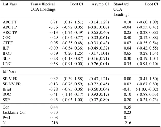
Table 3.4: Estimates for first canonical correlation and directions for white matter tract RD values and EF tests for transelliptical and standard CCA

DTI Vars Transelliptical

CCA Loadings Boot CI Asymp CI StandardCCA Loadings

Boot CI

ARCFT Left 0.93 (0.30, 2.06) (0.39, 1.47) 0.21 (-0.60, 1.09) ARCFT Right -0.83 (-2.53, 0.45) (-1.87, 0.22) 0.48 (-0.38, 1.77) ARCFP Left -0.26 (-1.18, 0.47) (-0.84, 0.32) 0.12 (-0.52, 0.86) ARCFP Right 0.24 (-0.38, 0.98) (-0.32, 0.81) 0.09 (-0.46, 0.67) ARCTP Left 0.05 (-0.62, 0.79) (-0.45, 0.56) 0.10 (-0.55, 0.85) ARCTP Right -0.05 (-1.06, 0.95) (-0.76, 0.65) -0.73 (-1.70, -0.27) CGC Left 0.25 (-0.51, 1.22) (-0.32, 0.82) 0.10 (-0.62, 0.83) CGC Right -0.02 (-0.84, 0.64) (-0.50, 0.47) -0.21 (-0.85, 0.30) CTPF Left 0.27 (-0.13, 0.84) (-0.12, 0.66) 0.11 (-0.27, 0.51) CTPF Right 0.17 (-0.28, 0.83) (-0.21, 0.56) 0.19 (-0.16, 0.69) Genu 0.02 (-0.64, 0.68) (-0.47, 0.51) -0.01 (-0.56, 0.53) ILF Left -0.04 (-0.92, 0.80) (-0.65, 0.57) -0.02 (-0.75, 0.68) ILF Right 0.26 (-0.45, 1.04) (-0.23, 0.76) -0.17 (-0.81, 0.35) IFOF Left 0.89 (0.12, 2.10) (0.19, 1.58) 0.75 (0.16, 1.84) IFOF Right -1.31 (-2.73, -0.52) (-1.89, -0.73) -1.10 (-2.27, -0.52) SLF Left -0.50 (-1.42, 0.26) (-1.06, 0.07) -0.05 (-0.73, 0.62) SLF Right 0.06 (-0.64, 0.72) (-0.47, 0.60) -0.12 (-0.89, 0.54) Splenium -0.66 (-1.39, -0.27) (-1.04, -0.28) -0.65 (-1.39, -0.33) UNC Left -0.26 (-1.09, 0.48) (-0.83, 0.32) -0.02 (-0.75, 0.70) UNC Right 0.64 (0.01, 1.54) (0.14, 1.14) 0.68 (0.23, 1.50) EF Vars

SB V FR 1.02 (0.71, 1.77) (0.86, 1.19) 0.87 (0.55, 1.57) SB NV FR -0.41 (-1.09, 0.22) (-0.94, 0.11) -0.50 (-1.30, 0.08) Brief -0.26 (-0.77, 0.10) (-0.59, 0.07) -0.54 (-1.18, -0.17) SOC -0.01 (-0.64, 0.58) (-0.44, 0.41) 0.14 (-0.40, 0.73) SSP 0.17 (-0.55, 0.91) (-0.24, 0.57) -0.18 (-0.79, 0.31)

Cor 0.63 0.48

Jackknife Cor 0.49 0.32

Pval 4.80E-04 4.138E-03

(49)

Table 3.5 reports the estimated first direction and correlation for transformed Kendall’s CCA and standard CCA. The jackknife corrected estimate for the first canonical correlation using transformed Kendall’s CCA is 0.33, compared to 0.23 for standard CCA. In this case only CCA using the transformed Kendall estimator has a p-value less than 0.05 for the first direction based on the bootstrap testing procedure. The first direction for the DTI lateralization measures is driven by positive loadings for the ARC FT and IFOF tracts. The first direction for the EF test cores is driven by a positive loading for the SB V FR scores. This indicates that higher lateralization score for the ARC FT and IFOF tracts is associated with higher SB V FR scores. A higher lateralization score means that RD is lower on the right hemisphere, indicating higher myelination for the right hemisphere tract. This gives evidence that for ARC FT and IFOF tracts greater development of the right hemisphere relative to the left hemisphere is associated with greater fluid reasoning. To the authors’ knowledge, this is a novel finding.

(50)

Table 3.5: Estimates for first canonical correlation and direction for RD lateralization measure and EF tests for transformed Kendall’s CCA and standard CCA

Lat Vars Transelliptical

CCA Loadings Boot CI Asymp CI StandardCCA Loadings

Boot CI

ARC FT 0.71 (0.17 ,1.51) (0.14 ,1.29) 0.18 (-0.60, 1.09) ARC FP -0.36 (-0.92 ,0.05) (-0.81 ,0.08) -0.04 (-0.55, 0.47) ARC TP -0.13 (-0.74 ,0.49) (-0.65 ,0.40) 0.25 (-0.28, 0.88) CGC 0.29 (-0.04 ,0.77) (-0.03 ,0.61) 0.40 (0.12, 0.88) CTPF 0.05 (-0.35 ,0.48) (-0.33 ,0.43) 0.07 (-0.35, 0.54) ILF -0.09 (-0.54 ,0.36) (-0.49 ,0.32) 0.04 (-0.42, 0.55) IFOF 0.59 (0.20 ,1.25) (0.17 ,1.01) 0.65 (0.28, 1.34) SLF 0.28 (-0.18 ,0.87) (-0.16 ,0.71) 0.30 (-0.19, 1.04) UNC -0.38 (-0.91 ,0.00) (-0.76 ,0.01) -0.35 (-0.94, 0.10) EF Vars

SB V FR 0.82 (0.39 ,1.58) (0.43 ,1.21) 0.80 (0.41, 1.50) SB NV FR -0.13 (-0.76 ,0.59) (-0.72 ,0.45) 0.02 (-0.67, 0.80) Brief -0.28 (-0.75 ,0.06) (-0.60 ,0.04) -0.41 (-1.03, -0.02) SOC -0.41 (-1.14 ,0.17) (-0.93 ,0.12) -0.10 (-0.88, 0.53) SSP 0.43 (-0.05 ,1.00) (0.07 ,0.80) 0.20 (-0.24, 0.73)

Cor 0.44 0.35

Jackknife Cor 0.33 0.23

Pval 0.03 0.11