Silverman_unc_0153D_17427.pdf

METHODS FOR THE SEQUENTIAL PARALLEL COMPARISON DESIGN

Rachel Kloss Silverman

A dissertation submitted to the faculty at the University of North Carolina at Chapel Hill in partial fulfillment of the requirements for the degree of Doctor of Philosophy in the Department

of Biostatistics in the Gillings School of Global Public Health.

Chapel Hill 2017

Approved by: Anastasia Ivanova Jason Fine

©2017

ABSTRACT

Rachel Kloss Silverman: Methods for the Sequential Parallel Comparison Design (Under the direction of Anastasia Ivanova and Jason Fine)

Sequential parallel comparison design (SPCD) has been proposed to increase the

likelihood of success of clinical trials, especially trials with a possibly high placebo effect. SPCD is conducted with two stages, and subjects are randomized into three groups: (1) placebo in both periods, (2) placebo in the first period and active therapy in the second period, and (3) active therapy in both periods. Efficacy analysis of the study data includes all data from stage 1 and all placebo non-responding subjects from stage 2. Each stage is analyzed separately then the data are pooled to yield a single p-value.

We first describe methods to use in a trial where we combine SPCD with the group sequential approach. We examine how to increase the sample size and adjust the design parameters during an interim analysis to increase power; these design parameters include allocation proportion to placebo in stage 1 of SPCD and weight of stage 1 data in the overall efficacy test statistic.

omit covariance in the construction of the overall test statistic and the confidence interval for the weighted sum of treatment effects.

We develop framework and implementation of SPCD using permutation tests and

To Justin, I could not have done this without you.

ACKNOWLEDGEMENTS

TABLE OF CONTENTS

LIST OF TABLES...ix

LIST OF FIGURES...x

CHAPTER 1: LITERATURE REVIEW ... 1

1.1 Overview ... 1

1.2 Next Chapters... 8

CHAPTER 2: SAMPLE SIZE RE-ESTIMATION AND OTHER MIDCOURSE ADJUSTMENTS WITH SEQUENTIAL PARALLEL COMPARISON DESIGN ... 10

2.1 Introduction ... 10

2.2 Simulations ... 13

2.3 Simulation Results ... 15

2.4 Discussion ... 17

CHAPTER 3: SEQUENTIAL PARALLEL COMPARISON DESIGN WITH BINARY AND TIME-TO-EVENT OUTCOMES ... 20

3.1 Introduction ... 20

3.2 Inferences in SPCD with Binary Outcomes ... 22

3.3 Time-to-Event Outcomes ... 26

3.4 ADAPT-A Trial Example ... 28

3.5 Simulation Study, Binary Outcomes... 30

3.6 Simulations, Time-to-Event Outcomes ... 32

CHAPTER 4: PERMUTATION-BASED INFERENCE

FOR SEQUENTIAL PARALLEL COMPARISON DESIGN ... 36

4.1 Permutation Test ... 36

4.2 Permutation test for SPCD ... 37

4.3 The Bootstrap ... 38

4.4 The Bootstrap for SPCD ... 38

4.5 Permutation and Bootstrap SPCD Simulation Study ... 41

4.6 Simulation Results ... 43

4.7 ADAPT-A Example ... 45

4.8 Stage-wise Testing in SAS... 46

4.9 Discussion ... 48

APPENDIX 1: FIGURES AND TABLES...50

LIST OF TABLES

Table 1. Simulated power for SPCD without sample size re-estimation, with sample size re-estimation alone, and with weight and allocation

re-adjustment for six scenarios. ... 54

Table 2. Asymptotic power for SPCD in six scenarios. ... 55

Table 3. Simulated power for SPCD in six scenarios. ... 56

Table 4. Estimated treatment effects, standard errors, and confidence intervals from ADAPT-A trial with analysis using unadjusted logistic regression model and with adjustment for center. ... 57

Table 5. Test statistics from ADAPT-A trial with analysis using unadjusted logistic regression model, logistic regression with adjustment for center, and the score test. ... 58

Table 6. Binary outcome – logistic regression with and without covariates. ... 59

Table 7. Time-to-event analysis – without covariate. ... 60

Table 8. Time-to-event analysis – with covariates. ... 61

Table 9. Type I error for normal, gamma, and Poisson distributed outcomes when the total sample size is 45, 60, and 90. ... 62

LIST OF FIGURES

Figure 1. Placebo lead-in study design. ... 50

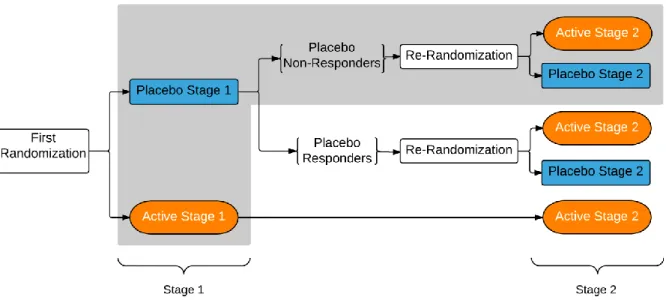
Figure 2. Sequential parallel comparison design. Outcomes highlighted

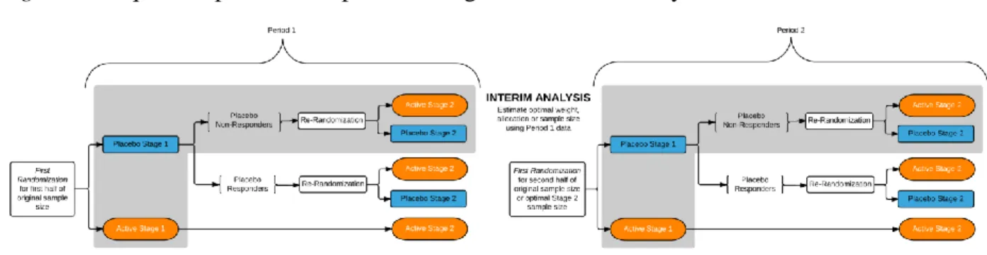
within the grey box are used in the efficacy analysis. ... 51 Figure 3: Sequential parallel comparison design with interim analysis. ... 52

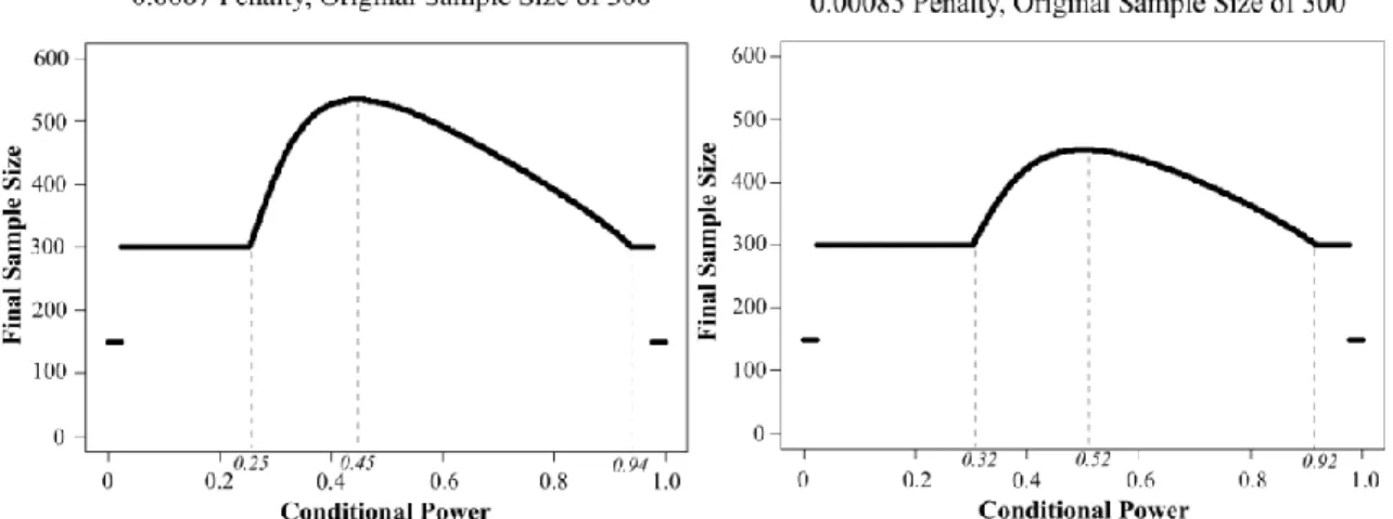
Figure 4. Rules for adding the sample size. Final sample size is plotted by conditional power for different penalty terms and originally

CHAPTER 1: LITERATURE REVIEW

1.1 Overview

The sequential parallel comparison design (SPCD) was developed to combat the issue of large placebo response rates that can occur in traditional randomized clinical trials (Fava, Evins, Dorer, & Schoenfeld, 2003). High rates of placebo response in clinical trials, even of drugs previously approved by the FDA for a particular condition, have often failed to demonstrate a significant difference in the active treatment from placebo (Baer & Ivanova, 2013). This failure arises because large placebo response rates that can occur in traditional randomized clinical trials will decrease the appearance of any true effect size and increase the likelihood of concluding a false-negative at the trial end or an outcome that is no longer clinically meaningful. Such a situation makes it necessary to increase the sample size to achieve the power that is necessary to conclude a true result. As these are extremely costly consequences, there are various trial designs devoted to reducing this placebo effect. In addition to the monetary ramifications of an extensive placebo response rate, there are additional public health implications. Negative results and failed trials can delay the introduction of new therapies on the market which, in turn, raises the cost of development or can cause companies to abandon development of treatments that are effective. In fact, some companies have decided to abandon their drug development efforts in certain fields, such as depression because the risk of an effective treatment failing to show efficacy is so high (Baer & Ivanova, 2013).

design (Figure 1), all patients first receive placebo, and then only those non-responding placebo patients are randomized to the placebo versus active therapy arms for the efficacy analysis treatment phase (Fedorov & Lui, 2007). Ultimately, the placebo lead-in design has been shown to be unsuccessful (Trivedi & Rush, 1994). In fact, on average, the use of the placebo lead-in approach often added time and cost to trials without increasing the effect sizes (Baer & Ivanova, 2013).

In 2003, Fava et al. proposed SPCD where subject assignment is as in a three-sequence, two-stage crossover design with PP, PA, and AA sequences where “P” stands for placebo and “A” stands for active therapy. SPCD takes a different approach to data analysis compared to a crossover design in order to avoid making assumptions about equality of treatment effects in the two stages. SPCD analyzes data from each stage separately and then combines the two analyses are combined to yield a single p-value. To avoid dealing with carry-over effects, SPCD does not utilize stage 2 data from the AA group. Additionally, subjects who responded to placebo in stage 1 (as determined a priori and by some clinically relevant cut point) are identified and their data are not included in the primary efficacy analysis. A more in-depth discussion of the trial design, implementation, and testing is provided later in this chapter. This design is useful in trials with high placebo response. SPCD might yield a higher power than a conventional single-stage design because (1) placebo non-responders contribute two data points to the primary efficacy analysis and (2) the exclusion of placebo responders in stage 2 might lead to an increased treatment effect in stage 2. Ivanova and Tamura (2011) extended SPCD by re-randomizing active treatment responders to P and A in stage 2.

dose-response studies. This advantage exists because, in these cases, it is difficult to recruit for these trials, and there is often a desire to generate adequate power while minimizing the investment or exposure of young people to new compounds. Additionally, SPCD can allow a sponsor to compare a new treatment at several alternative doses to placebo in the population of patients in stage 1, and to compare some of the doses in placebo non-responders in stage 2.

SPCD, when compared to the popular placebo lead-in trials, can be considered a more clinically relevant and generalizable trial (Baer & Ivanova, 2013). This is because SPCD trials give weight to the results of everyone enrolled in the trial. Furthermore, in clinical practice, the more resistant patients (placebo non-responders) seek treatment; therefore, a design that focuses on placebo non-responders can, in fact, address the population that new treatments seek to help. Thus, we can view stage 1 of SPCD as the generalizable stage and stage 2 as the more clinically realistic stage.

We can attribute additional merits of SPCD to the fact that an SPCD trial is typically longer than a placebo lead-in or a single-stage trial, with some patients staying on placebo or active drug therapy for the duration of the SPCD trial. This allows the trial sponsor and the FDA to obtain valuable data on response over time and additional safety measurements (Baer & Ivanova, 2013).

intervals for the weighted combination of the stage-wise treatment effects when the outcome is binary for SPCD. Data analysis strategies for SPCD with continuous outcomes can be found in Tamura and Huang (2007), Chen et al. (2011), and Doros et al. (2013). These researchers base the test statistic on the linear combination of the estimated treatment effects. It is possible to adjust for covariates, but such methods are not applicable to binary data. Baer and Ivanova (2013) reviewed data analysis methods for SPCD and summarized completed trials that used SPCD.

Specifically, the trial is conducted in two stages (Figure 2): randomization of all subjects to active therapy or placebo in stage 1 and then a re-randomization of stage 1 placebo non-responders in stage 2. Placebo non-responders are usually re-randomized in stage 2 as well and subjects who received A in stage 1 usually continue on A in stage 2. If randomization is conducted by flipping a biased coin, an equivalent format would be to randomize all subjects once at the onset of the trial into three groups: (1) placebo in stage 1 and placebo in stage 2 (PP); (2) placebo in stage 1 and active therapy in stage 2 (PA); and (3) active therapy in stage 1 and active therapy in stage 2 (AA). In this format, the primary analysis includes all stage 1 and stage 2 data from placebo non-responders from groups PP and PA. Irrespective of randomization format, all subjects are followed for the duration of both stages to maintain blinding.

Let the total sample size in the trial be n with n₁subjects in the placebo group, n₂subjects in the active therapy group in stage 1, n₁n₂ n, with n₁bn where b, 0 b 1, is the

have enough subjects to evaluate in stage 2. Allocation proportions above 0.75 are not

recommended because the design becomes very similar to the placebo lead-in design which has been shown to be ineffective in identifying placebo non-responders (Trivedi and Rush, 1994). Despite guidelines suggesting b between 0.50 and 0.75, b could be arbitrary. In stage 2, subjects are re-randomized to placebo and active therapy with 50:50 allocation.

For binary responses, denote p = Pr(active therapy response in stage 1), ₁ q₁= Pr(placebo response in stage 1), p = Pr(active therapy response in stage 2 | placebo non-responder in stage ₂ 1), and q = Pr(placebo response in stage 2 | placebo non-responder in stage 1). Let the treatment ₂ effects in stage 1 and stage 2 be defined as follows:  ₁ p₁q₁ and  ₂ p₂ q₂. We are

interested in testing the null hypothesis, H₀:₁ ₂ 0 with the alternative hypothesis that at least one of the treatment effects is different from zero. One possible approach to test

0: 1 2 0

H    is to combine tests of ₁ and ₂. This approach requires the knowledge of the correlation between the tests under the null hypothesis. Alternatively, one may consider the test statistic based on the weighted average of the estimated treatment effects as described. In

practice, we let (X Y_i, )_i be a pair of binary responses of subject i in stage 1 and stage 2 of SPCD, respectively. Then the estimated treatment effects are:

1 1 1 2 1 1 1 1 2

/ _i /

n n n

i

i i n

X

X n n



  

 





1 1

1

1 1

1 /2 1

/2

2 (1 ) / ( /2) (1 ) / ( / 2)

n n

i i i i

i i n

X Y n X Y n

  



 





With the SPCD test statistic,

1 2

2 2

1 2

I

(1 )

) 1 )

( ( ) (

w T

w Var V

where weight w, 0 w 1, is chosen a priori and based on the assumed stage-wise treatment effects, Var( ₁) ₁(1₁) / (n₁n₂) and 1

2 2 ₁

2

( ) (1 ) / n (1 _i)

i

Var   



1 2

1 ₁ / ( 1 2)

n n i

i X n n

 

 



2 ₁(1 ) / 1

n

i i i X Y n

 



Fava et al. (2003) proposed a similar test statistic, but derived the denominator was derived from the asymptotic distribution of a multinomial vector of counts in stages 1 and 2 of SPCD.

For continuous outcomes, the treatment effect in stage 1 of SPCD, D₁, is measured in the population of “all comers,” and the treatment effect in stage 2, D₂, is measured in the population of placebo non-responders. The null hypothesis isH₀:D₁D₂ 0 with an alternative hypothesis that at least one of the treatment effects is larger than zero. One approach to testing the

intersection null hypothesis is by using the weighted average of the estimated treatment effects,

1 (1 ) 2

ˆ _w ˆ

wD   D , where the weight w (0 < w < 1) is pre-specified (Chen et al., 2011).

We assume that responses from stages 1 (represented by X) and 2 (represented by Y) from patients assigned to placebo in both stages (PP group) of SPCD follow bivariate normal distribution:





2 2

2

, ~ P , P PP P ,

P P

P PP P P

X Y N    

   

    

    

 _{   }

 

and that responses from patients assigned to placebo in stage 1 of SPCD and active treatment in stage 2 (PA group) of SPCD also follow bivariate normal distribution:





2 2

, ~ P , P PA P A .

P A

A PA P A A

X Y N     

    

    

    

 _{   }

We further assume that responses of patients receiving active treatment in stage 1 of

SPCD are 2

1 ~ ( , )

A A A

X N   . Treatment effect for stage 1 is D₁_A1_P1. The stage 1 placebo group response probability is rPr(X_P c), where c represents the known response cutoff. The treatment effect in stage 2 is D₂ E Y{ _A|X_P  c} E Y{ _P|X_Pc}. The test statistic given by (Chen et al., 2011):

1 2

2 2

1 2

(1 )

( ) (1 ) ( )

SPCD

wD w D

w Var D w Var D

T  

 

 (1)

has a standard normal distribution T_SPCD ~ N(0,1) under the null hypothesis (Chen et al., 2011), and we reject the null hypothesis when T_SPCD 1.96. In some therapeutic areas that use SPCD (e.g., psychiatry), it is often more appropriate to examine the decline of symptoms and, as such, negative responses with large absolute value correspond to good treatment response. In this case, one would reject a one-sided null hypothesis when T_SPCD1.96. One can apply the methods described here to psychiatry trials after multiplying responses by (-1).

While the framework of SPCD with continuous and binary outcomes has been explored, we are not aware of published methods for the analysis of SPCD with time-to-event outcomes. Instead of comparing the number of occurrences between active therapy and placebo groups, one can evaluate the time to the first occurrence and determine if that time to the first occurrence is elongated or shortened on active therapy as compared to the placebo group. Alternatively, if a recurrent event is measured, one could estimate the mean cumulative function and answer questions about average number of events by some meaningful amount of time between placebo and active treatment groups (Lawless and Nadeau, 1995; Diao, Cook and Lee, 2015;

shorten the time to first event compared to placebo. Addyi (flibanserin) was FDA approved for the treatment of hypoactive sexual desire disorder

(https://clinicaltrials.gov/show/NCT00996164). The conducted trials compared Addyi to placebo by measuring the number of satisfying sexual events in the placebo and the active therapy arm. The baseline counts of satisfying events for the study participants were low, with 25-50% of participants having 0-1 events; as such, time to event could be a better endpoint to evaluate active treatment effect. The active-placebo comparison can be based on the average number of events as well as the time to the first event.

1.2 Next Chapters

We organize the remainder of this dissertation in the following way. For Chapter 2, our purpose is to evaluate various adaptive strategies in an SPCD trial with one interim analysis and continuous outcomes and to provide recommendations regarding their implementation in an SPCD trial. We consider five adaptive strategies in which we modify the following design parameters in period 2 with the goal of increasing the power of treatment comparison: (1)

possibly increase sample size; (2) possibly increase sample size, update the weight and allocation in stage 1 of SPCD with the weight, w*, and allocation, b*, that maximize power based on period 1 data; (3) update w and b, with w* and b*; (4) update w, with w*; and (5) update b, with b*. Additionally, in each of the strategies, we determine if we can stop the trial for futility or efficacy at the interim analysis.

adjusting for covariates and how to construct a confidence interval for the weighted combination of the treatment effects.

CHAPTER 2: SAMPLE SIZE RE-ESTIMATION AND OTHER MIDCOURSE

ADJUSTMENTS WITH SEQUENTIAL PARALLEL COMPARISON DESIGN1

2.1 Introduction

For a completely known distribution of responses in stages 1 and 2 of SPCD, one can compute the optimal pair of the weight, w, and allocation to placebo in stage 1, b, which

maximizes the power of the SPCD analysis. Since we cannot know the treatment effects before the trial (this is especially true for stage 2 treatment effects), one might consider utilizing a blinded interim analysis to estimate the treatment effects from both stages. Then we can compute the optimal pair of the weight and allocation and use that for the remainder of the trial with the intention to increase power. Alternatively, one can ensure adequate power for the trial by increasing the sample size based on the estimated effect sizes and the proportion of placebo non-responders. Mi and Betensky (2013) considered SPCD with binary outcomes with one interim analysis. They performed adaptations that (1) converted SPCD to a single-stage design if the stage 1 placebo response rate was small, (2) converted SPCD to a single-stage design if the stage 1 treatment effect was large, and (3) used sample size re-estimation. Their simulations showed that the type I error rate was inflated to as much as 0.06 when they performed each of the three adaptations was performed; therefore, they proposed an ad hoc adjustment of the critical value to preserve the type I error rate. Wang and Ivanova (2014) described a multi-arm SPCD trial with

1

an interim analysis to possibly drop some of the arms or change the allocation proportion to the arms, depending on the observed responses.

Interim analyses in an SPCD trial are conducted after a proportion (e.g., half) of the planned sample size has completed both stages of SPCD (Figure 3). It is desirable to conduct an interim look in order to check previous placebo response rates and treatment effect assumptions. Thus, if the previous assumptions were not correct, adaptations can be made to increase the power of the study. Let m be the number of subjects enrolled in the study before the interim analysis. We denote the study before the interim look as period 1, and the study after the interim look as period 2. We compute period specific test statistics for SPCD, T₁ and T_{2, for periods 1} and 2, respectively, using Equation 1 from Chapter 1. The final test statistic is (Lehmacher and Wassmer, 1999):

1 1 v 2

vT T

T    . (2)

Here, vm n/ , where n is the originally planned sample size. This test statistic is the same as proposed by Cui, Hung, and Wang (1999). If we perform an interim analysis after half of the subjects complete their follow-up, we set v = 0.5. In psychiatry, a typical SPCD trial has two stages, each 4 weeks long; hence, some subjects will be randomized while subjects 1,…, m complete their follow-up. T₁ and T₂ are independent, since T₁ is computed based on the data from subjects 1,…, m, and T₂ is computed based on the data from subjects m + 1, …, n. As a result,

~ N(0,1)

T and we reject the null hypothesis when T 1.96. (Ivanova, Li, Silverman, Wiener,

& Koch, n.d.)

trial was originally powered (Liu and Chi, 2001) as the observed treatment effect can be rather variable. In SPCD, little information is usually available about the second stage treatment effect, which is why estimated effects are used. There have been a number of proposals on how to set a new sample size(Gao, Ware, & Mehta, 2008; Jennison & Turnbull, 2015; Liu & Chi, 2001; Mehta & Pocock, 2010; Timmesfeld, Schäfer, & Müller, 2007; Wan, Ellenberg, & Anderson, 2015). The method proposed by Jennison and Turnbull (2015) maximizes an objective function:

* *

1

( ,t n ) (n )

CP  n . (3)

Here, T1 = t1 is the test statistic observed in period 1, n* is the new total sample size, CP

is a conditional power given the trend observed in period 1, and γ is a penalty parameter. The penalty parameter is set by the trial sponsor to achieve a trade-off between the cost of adding extra subjects and a power increase. The test statistic at the end of the trial, given period 1 data, is





and hence *

1

( ,t n ) P X( 1.96)

CP   , where X ~N( vt₁ 1vt₁ (n*m) / (nm),1). The new total sample size, n*, is the size that maximizes ₁ * *

( ,t n ) (n )

CP  n . One can also set n_max, the pre-specified maximum allowed total sample size, and choose n* such that *

max nn n . Mehta and Pocock (2010) proposed to increase the sample size when conditional power is in a certain range (i.e., “promising zone”) and set the new sample size n* such that *

1

( ,t n ) 0.8

specification of the penalty parameter. Smaller penalty terms yield more substantial sample size increases and hence higher power. Since effect size is not precisely known at the interim

analysis, one cannot guarantee a certain power at the end of the trial with any sample size re-estimation method.

2.2 Simulations

In period 1, the stage 1 weight, w, and the allocation proportion to placebo, b, are set to be equal to the commonly used stage 1 weight of w = 0.5 and allocation proportion of b = 0.67. To re-evaluate the weight and/or allocation to placebo in SPCD with an interim look, we utilize the data collected in period 1 (from subjects who have completed both stages of SPCD) to estimate the weight and/or allocation that would have produced the largest power in period 2 given the estimated treatment effects, variability of the outcome, and proportion of placebo non-responders. Thus, we found the optimal parameters w* and b* by maximizing the function

( 1.96 T_SPCD( , ))w b

   with respect to w, b, or both w and b. For computational simplicity, we used a grid search method and searched over [0,1] for optimal weight and [0.5,1) for optimal allocation. We then used these optimal weights and/or allocations in period 2.

We conducted an SPCD trial with an interim analysis with initial weight of w = 0.5 and the allocation to placebo in stage 1 of SPCD of b = 0.67. The total planned sample size was n = 300. We conducted the interim look after half of the subjects, n/2 = 150, were enrolled and had completed both stages of SPCD. We also considered trials with an interim look after 100 patients with total planned sample size of n = 200. Placebo non-response probability in stage 1 of SPCD was set to r = 0.75 in all scenarios except the final one where it was r = 0.60. We set the

yielding the variances of the outcomes in stage 2, conditional variances of 0.7 in placebo group, and 0.96 in active treatment group. A typical SPCD trial has two stages, each 3-5 weeks long; hence, we randomized some subjects belonging to period 2 at a time when an updated allocation was not yet available. Upon the availability of the updated allocation, one can set the new period 2 allocation to take into account several subjects randomized with initial allocation. Since the optimal weight is used in the calculation of the period 2 test statistic, there is no issue with any delay in the interim analysis. Therefore, we considered that all period 2 subjects were

randomized using the updated allocation. We simulated data with no dropouts. For the strategy in which we re-evaluated both allocation and weight, we selected the allocations to placebo in stage 1 from [0.5,1]. If we re-evaluated the allocation only, we examined allocations to placebo in stage 1 from [0.5,1), excluding 1. When an allocation to placebo was 1 in stage 1 of SPCD, it was equivalent to the placebo lead-in design. In that case, we based the analysis on stage 2 data only. Therefore, because the notion of weight no longer applied, we excluded 1 when we re-evaluated the allocation only. In all of the adaptive strategies, we considered stopping for futility and efficacy. We stopped for futility at the interim when T1 < 0. To stop for efficacy, we used the

O’Brien-Fleming boundary, performed an interim look after the first half of the trial, and stopped after period 1 if T1 > 2.7959. The final efficacy was established when T > 1.977 (Fleming,

2.3 Simulation Results

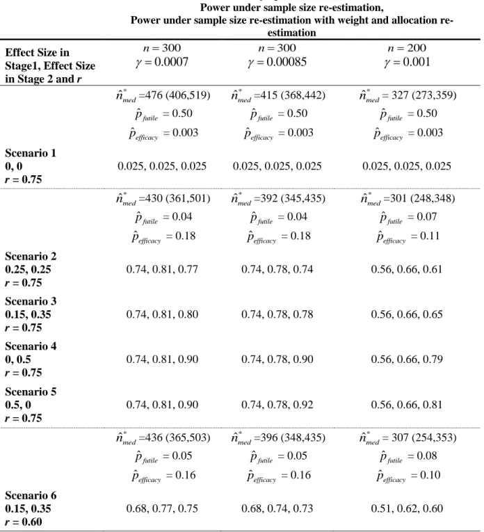
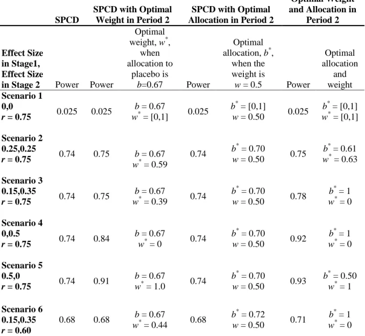
Table 1 displays the simulation results of SPCD with sample size re-estimation and sample size re-estimation with additional estimation of weight and allocation proportion to placebo (i.e., adaptive strategies (1) and (2) from Section 1.2). Scenario 1 is a null scenario. Figure 4 shows how the rules for the sample size increase at the interim analysis for several penalty parameters as a function of conditional power, CP. We selected the penalty term of 0.0007 because it attains 80% power in scenarios 2-5 in our simulation study. When designing a study, the penalty parameter can be chosen to yield a required power for potential efficacy scenarios. The penalty parameter can also be viewed as guiding a cost/benefit trade-off per each patient added.When the originally planned sample size is 300 and the penalty parameter is 0.0007, the sample size is increased for conditional powers of 25% to 94% (Figure 4), or,

alternatively, for T1 values between 0.93 and 2.49 with the maximum sample size increase to the

total sample size of 535 when conditional power is 45%. When the sample size is 300 and the penalty parameter is 0.00085, the sample size is increased for conditional powers of 32% to 92%, or, alternatively, for T1 values between 1.03 and 2.38 with the maximum sample size increase is

to the total size of 452 when conditional power is 52%. When the sample size is 200 and the penalty parameter is 0.001, the sample size is increased for conditional powers of 24% to 94%, or, alternatively, for T1 values between 0.91 and 2.53 with the maximum sample size increase is

the first 150 patients leads to a better-powered trial. The median total sample size after sample size re-estimation is 430 and 392 for a sample size of 300 and penalty terms 0.0007 and 0.00085, respectively. When the original sample size is 200, the median total sample size after sample size re-estimation with penalty parameter 0.001 is 301, yielding the power of 66% for scenarios 2-5. In comparison, when we used a fixed sample size of 300 is used, the power in scenarios 2-5 is 74%.

Re-estimation of weight and allocation together with sample size shows a further power increase, but not in all scenarios. For example, for scenarios 4 and 5, in which the original sample size is 300, after sample size re-estimation, the power is 81% and 78% for penalty parameters of 0.0007 and 0.00085, respectively. If we additionally re-estimate w and b, the power goes to 90% for scenario 4 (for both penalty parameters), 90% for scenario 5 (when the penalty is 0.0007), and 92% for scenario 5 (when the penalty parameter is 0.00085). In scenarios 2, 3, and 6, re-estimation of weight and allocation together with sample size decreases the gained power from the sample size re-estimation. This finding is a result of the initial weight and

allocation being close to optimal. As such, we see that re-estimating weight and allocation leads to selecting a sub-optimal weight and/or allocation.

To shed light on the advantages and disadvantages of re-estimating weight and allocation to placebo, we simulated the adaptive strategies (3), (4), and (5) (outlined in Section 1.2), fixed the sample size at 300, and re-estimated the weight and/or allocation. Table 2 shows the

unless the effect size in one of the stages is 0, in which case we can increase the power by using an optimal w or an optimal pair w and b. Interestingly, in the six scenarios we considered, there is no power benefit when using the optimal allocation alone while the weight remains w = 0.5; in fact, when we fix weight at 0.5, the optimal allocation for scenarios 1-5 is 0.70 and 0.72 for scenario 6. For this reason, we do not recommend this strategy or the strategy where the

allocation to placebo is updated alone with the sample size re-estimation. In scenario 4, when we adjust weight, the power can increase from 74% to 84% and further to 92% when we adjust both weight and allocation. In scenario 5, the power increases from 74% to 91% to 93%.

Table 3 shows the results from the corresponding simulations. For the scenarios where the initial weight and allocation were close to optimal (scenarios 2, 3, and 6), re-estimating the weight and/or allocation leads to selecting a sub-optimal weight and/or allocation and therefore to decreased power by 0-5%. When there is no treatment effect in one of the stages (i.e.,

scenarios 4 and 5), we can increase the power from 73% to 81% to 88% (as in scenario 4) or from 73% to 89% to 90% (as in scenario 5) when the weight is updated and when both the weight and allocation are updated.

2.4 Discussion

to improve power. As such, we advise using the default parameters in period 2 when treatment effects appear similar in both stages in period 1. We observed that changing the allocation alone did not lead to increased power in any of the scenarios; however, changing the weight can be beneficial. If the weight is changed and there is an interest in reporting the estimate of the weighted treatment effect wD1 + (1-w)D2 at the end of the trial, the estimate of this quantity can

be obtained for any given weight w using the four estimated treatment effects (from the two stages of SPCD for each of the two periods of the trial). For example, it might be beneficial, in order to preserve blinding, to always assign a certain proportion of patients to active arm in the first stage of SPCD, that is, to limit allowable allocation proportions to placebo to [0.5,.8]. As previously mentioned, SPCD generally has higher power than a single-stage design because some patients contribute two data points. We examined this potential increase in power through computing the expected value of the test statistic after the trial and extracting an equivalent effect size from it. For a single stage parallel arm trial, the expected value of the test statistic after a total of n patients complete the study is





0.3 300 / 2 , corresponding to an effect size equivalent of 0.3. Hence, one can think of SPCD as detecting an effect size of 0.25 as if it were an effect size of 0.30 (20% increase) in a traditional randomized clinical trial. Alternatively, one can think of SPCD as decreasing the sample size by a factor of 0.69 more than a traditional randomized clinical trial

since0.3 n / 20.25 1.22n / 20.25 1.44 / 2n .

longer due to the two-stage nature of the design; however, this aspect does not interfere with the successful application of these adaptive methods. In this paper, we examined continuous

CHAPTER 3: SEQUENTIAL PARALLEL COMPARISON DESIGN WITH BINARY AND TIME-TO-EVENT OUTCOMES

3.1 Introduction

A number of recent publications discussed crossover trials with time-to-event outcomes (Buyze & Goetghebeur, 2013; Makubate & Senn, 2010; Nason & Follmann, 2010). Care is needed when integrating the time-to-event endpoints into the SPCD framework. In each of the two stages, we define the time variable is defined as the time of event (for uncensored outcomes) or the end of follow-up for that stage (for censored outcomes). Stage 1 assesses this time-to-event endpoint for all randomized to active therapy or placebo. We consider the case where events are favorable and therefore regard as non-responders those subjects without events in stage 1. We would evaluate only those censored in the stage 1 placebo group in stage 2. As such, we condition the SPCD test statistic from stage 2 on a negative response (in this case, censored time) from stage 1. In fact, this setup is analogous to the case of SPCD with binary outcomes. Inferential results for continuous data are not applicable with time-to-event outcomes, owing to the specialized methods needed in the presence of right censoring.

Recall that with binary outcomes, the SCPD test statistic is as follows:

1 2

2 2

1 2

I

(1 )

) 1 )

( ( ) (

w T

w Var V

w ar w          ,

where weight w, 0 w 1, is chosen a priori, V ra ( ₁) ₁(1₁)(1 /n₁1 /n₂) and





1

/2

2 2 ₁

2 _{/2 1}

( ) (1 ) 1 / n (1 _i) 1 / n (1 _i)

i X i n

Var   





1 ₁ / ( 1 2)

n n i

i X n n

1 1

2 1(1 ) / 1(1 )

n n

i i i

i X Y i X

 





defined here are valid test statistics to test the SPCD null hypothesis that preserve the type I error rate under the null hypothesis.

The most common approach to adjust for covariates is to fit a logistic regression model to stage 1 SPCD data and separately to stage 2 SPCD data to test the null hypothesis

0: 1 2 0

H    , where ₁ and ₂ are log odds ratios in stages 1 and 2. Let ˆ₁ be the estimated log odds ratio from the stage 1 logistic regression model, and T₁ be the test statistic based on ˆ₁. Similarly, ˆ₂ and T₂ are the log odds ratio and the test statistic from stage 2 of SPCD. Consider the following test statistics:

1 2

2 2

1 2

II

(1 ) ) (1 )

( ( )

w T

w Var V

w ar w          ,

III 1 1 2

T  vT  vT .

In the above, Var( )1 and Var(2) are the corresponding elements of the asymptotic variance-covariance matrix that is computed as the inverse of the Fisher information. The weight v, 0 v 1 should be chosen in advance and plays a similar role to the weight w in TI and TII.

To address which test statistic, TIIor TIII, yields better power, we examine the optimal

weights w* and v*. Writing TII as:

1

1 2

2

2 2 2 2

1 2

II

2 1

) (1 ) )

) (1 ) )

( (

) (1 ) )

( ( ( (

w Var Var

T

w Var Var w V

w T ar Va w r T w             

illustrates the connection between the two test statistics. Given observed data, one can choose the optimal weights w* and v* so that max(T w_II( ))max(T_III( ))v T w_II( *)T_III( )v* . This

interested in finding the optimal weight to maximize power, we consider the case when T₁0 and T₂ 0. It is easy to see that when T₁0 and T₂ 0, the optimal weight for T_III is

* 2 2 2

1 / ( 1 2 )

v T T T . The optimal weight, w*, for TII can be obtained from the equation:

1

* 2

1 2 2

* *

1 1 2

2 2 2 ) ) (1 ( ( ) ( )

w Var T

T T

w Var w Var



      ,

* 2

1 2 2

2 1 ) / ) / ) / ( ( ( Var w

Var Var T

T T



  

 .

The weights w and v should be chosen in advance. However, the formulas for w* and v* can be useful if an investigator has prior knowledge about treatment effects and their variability in the two stages of SPCD.

In the next section, we will show that the treatment effect estimates from the two stages are uncorrelated and that any of T_I, T_II, and T_III are asymptotically mean zero under the null hypothesis and can be used to test the SPCD hypothesis.

3.2 Inferences in SPCD with Binary Outcomes

Let

1

1

( ,..., )

P X Xn

X be a vector of responses of subjects assigned to placebo in stage 1, and

1

1

( ,..., )

P Y Yn

Y be a corresponding vector of stage 2 responses. Let

1 1 1 2

( _n ,..., _{n n} )

A  X  X 

X

be a vector of responses of subjects assigned to active therapy in stage 1, and

1 1 1 2

( _n ,..., _{n n} )

A Y  Y 

Y be the corresponding vector of stage 2 responses. Define all stage 1 data as ,

( _{P A}) 

participants n₁1 through n₁n₂ as their stage 2 data are not included in the primary analysis. We consider the inferential issues associated with combining test statistics and treatment effect estimators from the two stages with binary data.

Consider a function (f X Z, ) of stage 1 data, which may involve stage 1 responses and baseline covariates. This can be an estimated treatment effect or test statistic, potentially adjusted for covariates. Since our analysis only includes stage 2 data from stage 1 placebo

non-responders, the stage 2 test statistics and treatment effect estimates are functions not only of stage 2 responses but also of stage 1 responses, denoted by a function ( , , )g X Y Z of data from both stages. It is important to recognize that the stage 2 analysis is based on the conditional distribution of Y given X and potentially Z. Thus, with binary data, the full likelihood function based on both stage 1 and stage 2 data factors into the stage 1 likelihood based on the marginal distribution of the stage 1 responses and the stage 2 likelihood based on the conditional distribution of the stage 1 responses given the data observed at stage 1. Such likelihood

factorization does not occur with continuous outcomes when response is defined by dichotomizing the continuous response. The lack of factorization in the case of continuous outcomes arises because the distribution of the stage 2 data conditions on an event that subject’s stage 1 outcome belongs to the set of stage 1 placebo non-responders and not the underlying continuous outcome itself. Factorization of the likelihood, and the fact that the expectation in stage 2 of SPCD is conditioned on the stage 1 outcomes, allows us to write:













cov( ( , ), ( , , )) ( , ) ( , , ) ( , ) ( , , ) | ,

( , ) ( , , ) | , [ ( , ) 0] 0.

f g E f g E E f g

E f E g E f

 

 _{  }

 

 _{ }  

X Z X Y Z X Z X Y Z X Z X Y Z X Z

X Z X Y Z X Z X Z

Let f(X Z, )n1/2(₁₁) and g(X Y Z, , )n*1/2(₂₂), with * 1

1

n

i i

n 



that when considering the distribution of the appropriately standardized _j , under the

alternative, for each fixed value of βj, the functions (f X Z, ) and ( , , )g X Y Z are not functions of unknown βj and are mean zero when βj is equal to the true value of the parameter, for j = 1, 2. Under the usual regularity conditions, the standardized maximum likelihood estimators

1/2

1 1

( , ) ( )

f X Z n   and g(X Y Z, , )n*1/2(₂₂) have an asymptotic multivariate normal distribution for all values of ₁ and ₂. When ₁ and ₂ are true parameter values,

asymptotically, the stage 1 quantity is unconditionally mean zero and the stage 2 quantity is mean zero conditioned on the results of stage 1. When g(X Y Z, , )n*1/2(2 2)0, asymptotically, using the above result, cov( (f X Z, ), ( , , ))g X Y Z 0 and the vector





1/2 *1/2

( ), ( )

n   n   converges in distribution to bivariate normal with mean zero and a

diagonal variance-covariance matrix. Hence, the covariance of the asymptotic distribution of ₁ and ₂ is 0. Because the treatment effect estimators from the two stages are asymptotically normal and uncorrelated, they are independent. A similar argument can be made when (f X Z, ) and ( , , )g X Y Z are test statistics as long as E g





(2) In the presence of covariates, the estimated logistic regression coefficients ˆ₁ and

2 ˆ

 are uncorrelated under the null and alternative hypotheses. As a result of potentially differing sample sizes in each stage, it is important to note here that all parameter estimates are standardized, that is, 1/ 2

1 1) (

n   and * 1/2 ₂ 2

( )

n    . (3) The test statistics T1 and T2 computed at stages 1 and 2, respectively, are

asymptotically uncorrelated under the null hypothesis.

The standardized test statistics are only mean zero under the null hypothesis and not the alternative hypothesis. Note that if we center the test statistics around their mean, they will be uncorrelated. The standardized treatment effect estimators are mean zero for fixed values of the β1 and β2 under both the null and alternative hypotheses. Having shown that the standardized

estimators are asymptotically normally distributed and uncorrelated for all values of the parameters, we can then use the delta method to establish the asymptotic normality of the

weighted combination of the estimators (after standardization) and derive its variance. This result enables the construction of confidence intervals which are valid under both the null and

alternative hypotheses.

Specifically, we have the following:

(1) The distribution of each standardized T_I, T_II, and T_III is asymptotically N(0,1) under the null hypothesis;

(2) The confidence interval





2 2

1) ( ) 2)

( 1 (

1) ˆ1 ˆ1) 1 ˆ1 ˆ1 2 ( (1 /n q(1 q) / Var   p p   n ,

1 1

1

/2

2 2 ₁ 2 2 _/

2) ˆ ˆ ) / (1 ˆ ˆ ₂

( (1 n _i) (1 ) / n (1 _i)

i i n

Var   p p





where 1

1 ₁ 1

ˆ n_i Xi /n

p 



1 ₁ 2

ˆ n n _i/

i n

q 



1/2 1/2

2 ₁ (1 ) ₁ (1 )

ˆ n _{i i}/ n _i

i Y i X

p 





1 1

2 _{/2 /2}

ˆ n (1 _i) _i/ n (1 _i)

i n i n

q 





The confidence interval (w₁ (1 w)₂Z_1/2SE,w₁ (1 w)₂Z_1/2SE) for

1 (1 ) 2

w  w has the coverage of 1. Here ₁ and ₂ are the log odds ratios and

2 2

1) ( ) 2)

( 1 (

SE w Var   w Var  .

3.3 Time-to-Event Outcomes

Under the SPCD setting, we define time-to-event outcomes in the classical way for both stages 1 and 2, and censoring for each stage occurs at the end of the stage. Let (1)

i

T be subject i's first event time in the first stage of SPCD. If the subject does not have an event until the end of stage one, the subject is censored at the end of stage 1. Let C_i(1) be the subject’s censoring time in stage 1, (1) (1)

i i

i

X T C be the observed stage 1 time for the subject, and (1) (1) (1)

( _i )

i I T Ci

   be

the indicator of whether the event was observed in stage 1. Let Z_i be the subject-specific vector of baseline covariates. Thus, the observed data for subject i in stage 1 are {X_i,_i(1),Z_i}. Let T_i(2) be subject i's event time in the second stage of SPCD where the time starts from the beginning of stage 2. Similarly to stage 1, if the subject does not have an event until the end of stage 2, the subject is censored at the end of stage 2. Let (2)

i

C be the subject’s censoring time in stage 2, (2) (2)

C

i i

i

Y T  be the observed stage 1 time for the subject, and (2) (2) (2)

( i )

i I T Ci

   be the

stages to maintain blinding, but primary analysis in SPCD only includes stage 2 data from subjects who did not respond to placebo in stage 1. Thus, we include only data from subjects assigned to placebo in stage 1 with X_i C_i(1) in SPCD primary analysis. Therefore,

(1) (2)

(X_i,_i , ,Y_i _i ,Z_i) are the full data of subject i in stage 1 and stage 2 of SPCD. The vectors of responses for each treatment group and stage are defined similar to the binary case.

A popular choice in evaluating the time-to-event data is the Cox proportional hazards model (Cox, 1972). The model is ( |t Z_i)₀( ) exp{t Z_i} where ₀( )t is the baseline hazard and  is the hazard ratio for active treatment versus placebo. To analyze SPCD data, we can consider stage-wise Cox models without or with covariates:

0

( | ) ( ) exp{ (Treatment Active)}

j t i j t jI j

 Z    , or

0 (Trea

( | ) ( ) exp{ tment Active) }

j t i j t jI j j i

 Z     Z .

We are interested in testing the null hypothesis that the treatment effects from both stages are zero, H₀:₁₂ 0. Similarly to the binary data setup, with time-to-event outcomes, test statistics and treatment effect estimators computed at stage 2 are evaluated conditionally on the stage 1 results. That is, ₂ refers to the hazard ratio for active treatment versus placebo

conditionally on an event not occurring during the stage 1 follow-up. One may argue along the lines in Section 3.2 to show that the likelihood function for the stage 1 and stage 2 survival outcomes factors under our definition of response and thus the estimated regression parameters based on partial likelihood are the maximum likelihood estimators based on separate estimation using the stage 1 and stage 2 data. As a result, the test statistics derived from the partial

bivariate normal and uncorrelated under both null and alternative hypotheses. The test statistics and parameter estimates may be combined, as with binary outcomes, with the theoretical properties of the weighted combination derived from the delta method. Analogous results in Section 3.2 will also apply to count data (e.g., Poisson type outcome) as long as the definition of placebo non-responder is a subject with no events.

To test the SPCD null hypothesis, we can use the weighted average of the estimated treatment effects, w₁ (1 w)₂ , where 0 w 1 and is chosen a priori, with the following test statistic:

1 2

IV

2 2

1 2

(1 ) ) (1 )

( ( )

w T

w Var V

w ar w

 

 

   

 .

Alternatively, we can use the test statistic T_V  vZ₁ 1vZ₂, where T1 and T2 are

stage-wise test statistics. These test statistics can be for testing the coefficients ₁ and ₂ in the Cox model, or, for example, can be stage-wise log-rank test statistics.

3.4 ADAPT-A Trial Example

ADAPT-A trial was a clinical trial to assess the efficacy of low-dose aripiprazole added to antidepressant therapy in patients with major depressive disorder and inadequate response to prior antidepressant therapy (Fava et al., 2012). SPCD was used with two stages of 30 days each. In the first stage, 167 patients were randomized to placebo and 54 to aripiprazole (3:1

patients responded to aripiprazole, and 29 out of 167 (17.4%) responded to placebo. Including stage 2 data from stage 1 placebo non-responders into the primary analysis yields the following counts in stage 2: 14 out of 65 (21.5%) patients responded to aripiprazole, and 5 out of 65 (7.7%) responded to placebo. The primary analysis reported by Fava et al. (2012) used binomial

repeated-measures regression, accounting for correlation between subject data in stages 1 and 2. The model was analyzed using SAS Proc Genmod (with identity link, binomial repeated

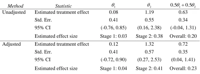
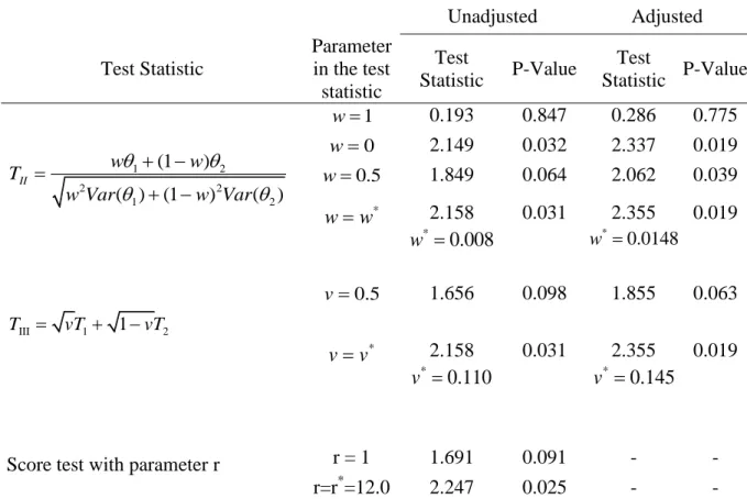
measures) and included study stage, treatments and their interaction, and control for categorical study center variables as randomization was stratified by center. In contrast, our method allows for performing stage-wise analyses and then combining either the estimated treatment effects or the test statistics without a need to estimate correlation between estimates in the two stages. Since there were a total of 21 centers, for the sake of this illustration, we combined the centers creating two larger centers. We performed stage-wise logistic regression analysis unadjusted and adjusted for center (Tables 4 and 5).

the discussion about optimal weights in Section 2.1, we computed optimal weights given observed data and corresponding test statistics. As discussed earlier, if the optimal weight computed based on observed data is used, the two test statistics are exactly the same. Table 5 also shows the results for the score test (Ivanova et al., 2011) with default parameter r = 1 and with the optimal parameter computed from observed data. The optimal parameter is equal to the ratio of the treatment effects *

(14 / 65 5 / 65) / (10 / 54 29 / 167) 12.0

r     .

We see in Table 4 that the effect size, defined as the treatment effect divided by the pooled standard deviation, is close to zero in stage 1, equaling to 0.03 and 0.04 for the

unadjusted and adjusted analyses, respectively. Clearly, using a single-stage design would give the impression that there is no benefit to low-dose aripiprazole in reducing the MADRS score. In contrast, the effect size is substantial in stage 2 with 0.38 for unadjusted and 0.41 for adjusted analyses, respectively. Since the treatment effect is much higher in stage 2 of SPCD, one might argue that the placebo lead-in design would have led to an even smaller p-value if used in ADAPT-A trial. This is because it would have had all patients assigned to placebo in stage 1, resulting in more subjects contributing to the primary analysis in stage 2. However, the placebo lead-in design might not have been as effective as SPCD in identifying placebo non-responders and increasing the treatment effect in stage 2 (Trivedi & Rush, 1994) resulting in a smaller treatment effect in stage 2. Also, if stage 1 treatment effect is slightly higher than observed in ADAPT-A trial, the SPCD is more powerful than the placebo lead-in design due to combining data on treatment comparison from both stages.

3.5 Simulation Study, Binary Outcomes

and 80 show that type I error is preserved even when the sample size is low. Data were generated using the inverse logit function with pre-specified treatment effect and covariate parameters. The correlations from the observations from the same subject were set to ρPP = 0.8 and ρPA = 0.3. The

covariate is assumed to be normally distributed and increases the odds of an event by 22% with a unit increase in the covariate (corresponds to a logistic regression parameter of 0.2). Simulation results are based on 150,000 runs. All tests were two-sided with a significance level of 0.05 and were conducted in R version 3.3.1.

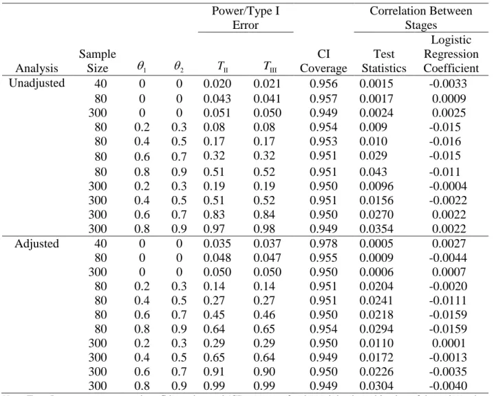
Table 6 displays the results of SPCD with binary outcomes with and without adjustment for covariates. In both cases, type I error is maintained at 0.05. Coverage of the 95% confidence interval for the overall treatment effect, defined as the weighted average of stage 1 and stage 2 treatment effects, is maintained for all scenarios. To verify the uncorrelatedness of stage 1 and 2 analyses, we estimated the correlation between the estimated treatment effects in the two stages of SPCD. With M simulation runs, the standard error for the estimated correlation is

2

(1 ) / ( 2)

3.6 Simulations, Time-to-Event Outcomes

In each simulation, both stages 1 and 2 were 28 days long, and stage 1 allocation to placebo was b2 / 3. The sample size was 300 for all scenarios with additional null simulations having sample sizes of 40 and 80 to show that type I error is preserved even when the sample size is low. We used exponential distribution with a scale parameter of 0.01 to simulate time to event on placebo in stage 1, yielding a stage 1 placebo response rate of 25%. We chose the exponential distribution to help uphold the proportional hazards assumption, which is not an unreasonable assumption when the stages are short in duration as in SPCD. A placebo non-responder is a subject who did not have an event in the first 28 days. Since having an event is a favorable outcome, active therapy is expected to reduce time to event compared to placebo. We sampled time to event in stage 1 in both the placebo and active therapy group using the inverse probability method proposed by Bender, Augustin, and Blettner (2005). This method ensures that the time to event follows the proportional hazards model assumptions. We censored all stage 1 times at 28 days. For those placebo non-responders re-randomized to placebo in stage 2, their stage 2 times to event were calculated as 28 days less than their original time to event. Thus, in the PP group, Y_P  X_P28 1 _P . This makes intuitive sense, as nothing has changed for these subjects. Times to event for placebo non-responders that are re-randomized to active therapy in stage 2 were calculated as, YP exp{₂I(Treatment₂ Active)}(XP28 1 ) P . These subjects,

and 8 report the results of these simulations with and without a covariate. Simulation results are based on 150,000 trial runs. All tests were two-sided with a significance level of 0.05.

As in the binary outcome simulations, the type I error rate is preserved. The 95%

confidence interval of the overall treatment effect provides correct coverage with 95% coverage for all scenarios both without and with covariates (Tables 7 and 8). The estimated treatment effects from stages 1 and 2 are uncorrelated under both the null and alternative hypotheses as expected. The results also confirm the uncorrelatedness of the stage-wise log-rank statistics under the null hypothesis but not under the alternative hypothesis, where the estimated mean correlation is outside the interval (-0.005,0.005), indicating that the true correlation is not 0.

3.7 Discussion

SPCD is an efficient design for comparing a novel intervention with placebo. Similar to a crossover design, it utilizes two data points from subjects, though not from all subjects as in a crossover, instead of one data point as with a standard trial design. Unlike crossover, one does not need to worry about the carry-over effect to analyze SPCD data as there is no required assumption about the relevant magnitude of treatment effects in the two stages. Researchers propose SPCD for trials with high placebo response because they believe it eliminates placebo responders from stage 2 and leads to higher treatment effect in stage 2. This, combined with the ability to collect two data points from subjects, in general, leads to a higher power of SPCD compared to a standard trial. One disadvantage of SPCD is that not all data are used in the primary analysis. For example, data of subjects who received active treatment in stage 2 are not utilized. These data, however, allow for important secondary analysis. For example, one can compare placebo and active treatment for the duration of the two stages of SPCD by comparing the responses from PP and AA groups at the end of stage 2.

For normal outcomes, many authors have proposed combining treatment effects with weights for the primary SPCD analysis. Chen et al. (2011) showed that the covariance between the estimated treatment effects is zero under the null hypothesis and, therefore, can be omitted in the denominator of the test statistic based on the weighted combination of the estimated

CHAPTER 4: PERMUTATION-BASED INFERENCE FOR SEQUENTIAL PARALLEL COMPARISON DESIGN

4.1 Permutation Test

Let U(u₁,...,u_n) and V (v₁,...,v_m) be two independent random samples, potentially drawn from two different distributions, F and G. The two-sample permutation test tests the null hypothesis, H₀:F G. Let N represent the combined sample of U and V of size nm. Additionally, let Z ( , )U V and Z' be the ordered vector of size N of all the data. Let

1,..., )

( N







belongs to. We have that ˆ  f( , Z) u v where u and v are the computed means of the

observed samples of U and V . All





! !

N N

n m n m

  

  _

  permutations of  are equally likely

under the null hypothesis that FG. We denote * as any one of these permutations of  and

can compute all N n    

  permutation replications of ˆ

 as  ( *) f(*,Z'). This provides the

permutation distribution of ˆ, and the probability that * exceeds ˆ represents the permutation significance level. Measuring the observed test statistic in relation to the null distribution

provides the exact p-value for the test. Thus, we can reject the null hypothesis at the 0.05 significance level when * ˆ) 0.05

the data. Dwass (1957) proposed using “modified randomization tests” which randomly samples a subset of reference datasets from the set of all data permutations to provide a valid test. The validity of the test is maintained even when the subsets are small in comparison to the possible number of permutations.

4.2 Permutation test for SPCD

Let n n₁, ₂ and n₃ be the stage 1 sample sizes for the PP, PA, and AA groups, respectively. For the PP group, let

1

1

( ,..., )

PP  X Xn

X be a vector of stage 1 responses, and

1

1

( ,..., )

PP  Y Yn

Y a corresponding vector of stage 2 responses. For the PA group, let

1 1 1 2

( _n ,..., _n )

PA X  X n

X be a vector of stage 1 placebo responses, and

1 1 1 2

( _n ,..., _n )

PA Y  Y n

Y a

corresponding vector of stage 2 active treatment responses. For the AA group, let

2 2 3

1 1 1

( _{n n} ,..., _{n n n} )

AA X   X  

X be a vector of stage 1 active treatment responses, and

2 2 3

1 1 1

( _{n n} ,..., _{n n n} )

AA Y   Y  

Y be the corresponding vector of stage 2 active treatment responses.

Also, let X_P(X_PP,X_PA) and Z (X_P,X_AA,Y_PA,Y_AA) be the collection of all the study data. We assume that XP and YPP are sampled from some probability distribution F and that

,

AA AA

X Y and Y_PA are sampled from some probability distribution G. We are interested in testing the null hypothesis that H₀:FG.

Here, Z' is a vector of size n of the ordered data, and  is the corresponding group assignment (P or A) vector of size n for Z'. We choose B independent vectors,





each consisting of n₁ PP’s, n₂ PA’s, and n₃ AA’s, from the set of all

1 2 3 N n n n

 

 _{ } 

  potential