TECHNICAL UNIVERSITY OF CLUJ-NAPOCA
ACTA TECHNICA NAPOCENSIS
Series: Applied Mathematics, Mechanics, and Engineering Vol. 62, Issue I March, 2019
MATRIX EXPONENTIALS IN ROBOT ELASTOKINEMATICS
Iuliu NEGREAN, Adina CRIŞAN
Abstract: The main objective of this paper consists in the establishment of the generalized elastokinematics equations
for robot structures with flexible links. For kinematics and differential matrices in the case of the robot structures with rigid and elastic links will be applied the matrix exponentials, in accordance with the algorithm developed by the main author. Consequently, the matrix exponentials will stay at the basis of establishment the linear and angular transfer matrices. By means of the same matrix exponentials will be also determined all kinematic parameters. In the second part of this paper elastokinematics structure of the serial robot will be analyzed. Applying the properties of the matrix exponentials, the locating matrices and their time derivatives corresponding to small deformations will be also established. On the basis of these differential transformations, in the final part of the paper, will be determined the linear and angular velocities and accelerations, as well as Jacobian matrix.
Key words: elastokinematics, elastodynamics, advanced mechanics, robotics.
1. INTRODUCTION
According to [2] – [7], transfer equations of any kinematic chain, with (R)-rotation or
(T)-prismatic joints, typical of MRS can be expressed WITH the locating transformations. The locating term substitutes the position and orientation between two kinetic links, shown in the Fig.1 and Fig.2. For analyze the transfer equations the mechanical robot structure (MRS)
is represented in the initial configuration:
T
i
0 q 0;i1n
. In the robot
kinematics the linear and angular transfer matrices will be defined, in the following, by means of matrix exponentials. As a result the DKM Equations answerable to linear and angular velocities and accelerations will be presented by their defining expressions. Considering these transfer matrices, in the following, the study with matrix exponentials will be extended about robotic structures with flexible links. The kinematic transformations for structures with rigid and elastic links will be compulsively applied in the second part of this paper devoted to the establishment of the elastokinematics equations. In the view of this, new formulations about matrix exponentials and
2. LINEAR TRANSFER MATRICES
In this section, according to [8]-[19] and [21], the expressions from the MEK Algorithm (MEK―Matrix Exponentials in Kinematics)
will be presented. At beginning, the partial derivative, with respect to qi of the locating
matrix between 0 n is established as:
i i n 0
n0 ii 1 i n
i 1 1
i 1 i
0 U q
jj 1 jj 1 jj 1
j 1 j 1
1
i i
0 0
jj 1 jj 1 jj 1
j 1 j 1
T T T q
T e E
where E T T
; (1)
0
jj 1 jj 1 4
where T ; i 2 ; I ; i 1
x
x 0 x 0 ii 1
i 1 n
0 i i x 0 i 1
R p
T T
0 0 0 1 exp A q T where x n ; n 1
; (2)
n
0 0
x 0 i i i x 0 i 1
R exp k q R
i 1 n 0j j i j
i 1 j 0 n
0 0
i i x i
i 1
exp k q b
p
exp k q p
xwhere 0; xn ; 1; x n 1
n0 ni ni
i
T A R A p
q 0 0 0 0
(3)
i 1 n
0 j j i k k n
j 0 k i
exp A q A exp A q T
The last column from (3) is taken into account for establish the exponential of the linear transfer matrix. According to [3], first and second matrix exponential from (3) shows as:
i 1
j j j 0
exp R exp p exp A q
0 0 0 1
; (4)
i 1 0 j j j j 0 i 1 i 1 0k k j 1 k
j 0 k 0
where exp R exp k q , and
exp p exp k q b
n k k k k k iexp R exp p exp A q
0 0 0 1
; (5)
n
0
k k k k
k i k 1 n
0
k m m m k
k i m i 1
where exp R exp k q , and
exp p exp k q b
;
m 0; m i 1 ; 1; m i
.
In keeping with the transfer matrix algorithm [5], it is known that the ith column from the linear transfer sub-matrix will represent the last column from (3) expression:
0i iv n ni i i 1 0 0 j j j i j 0 n 0 0
k k n k
k i i 1
0 0
i j j j i mk j 0
k 1 n
0
mk m m m k
k i m i 1
V J p A p
q
exp k q v
exp k q p
exp k q k A ,
and A exp k q b
. (6)Considering [4] and [6], the linear component
iv 0J
can be written under another matrix form:
i 1 0i1 j j j 3 x 3
j 0
ME V exp k q
; (7)
0 i2 3 i i 3 6ME V I k
; (8)
0T T n T k T 0 i 1 i n 3 9 iv p 3 i k ; b vM
; (9)
3 i 3
i 322 i 323 6 x 9 3 n i
I 0 0
ME V
0 ME V ME V
; (10)
k 1 0m m m m m i 1
i 322
m
exp k q
ME V
where k i n 0 ; m i 1 ; 1; m i
n
0
i 323 k k k
k i
ME V exp k q
.The above expressions are swinging for:i1n. So, the exponential of the linear matrix0JV
V , from Jacobian matrix
J
0
, will be characterized by the expression:
0 V 0 iv 3 x 3i1 i 2 i 3 iv
V J
J where i 1 n ME V ME V ME V M
. (11)
Remark: The second expression from (11) is
matrix one. It can be easily applied in the DKM generalized algorithm. As a result, this will dignify a few advantages of the matrix calculus.
3. ANGULAR TRANSFER MATRICES
In keeping with MEK Algorithm from [8]-[19] and [21], at beginning, the first time derivative for the exponential (2) of the locating matrix between 0 n is defined, that is:
i 1 n 0
n0 j j
n
i 1 j 0 n
0 i i k k n0
k i
T T exp A q A
where A A q exp A q T
& & & ;(12)
1 1
0 1 1 0
n0 n0 i i
n
i n
and T T T exp A q
.Performing the matrix product between the two matrices from (10), the expression is obtained:
0 1
0 1
n n n0 n0 i 1
n
j j i j i 1 j 0
0
j j j i
j i 1
T T T T
exp A q A A
where A exp A q q
& & &; (13)
0 0 1 1
n0 n0 n n
i i
i 1 0
j j i j j
j 0 j i 1
T T T T
q q
exp A q A exp A q
The inverses of the exponentials (4) and (5) are characterized by the following expressions:
1
n 1
i i i i
i 1 i n
i i
exp A q exp A q
exp R exp p
0 0 0 1
. (14)
1
0
i i i i
i n i i
0
i j j j i
i n j n
where exp R exp k q , and
exp p exp k q b
.In keeping with MEK Algorithm, to above expressions another is compulsory added:
i 1
j k
j j j 0
exp R exp p exp A q
0 0 0 1
; (14)
i 1 0j j j j
j 0 i 1 i 1
0
k k k k j 1
j 0 k 0
where exp R exp k q , and
exp p exp k q b
; 0 k k j j j i 1exp R exp p exp A q
0 0 0 1
.(15)
0 0k j j j
j i 1 j 0
0
k k k k j
j i 1 k i 1
where exp R exp k q , and
exp p exp k q b
.The skew-symmetric matrix associated to column vectori of the angular component from the velocity transfer matrix is the result of the following partial derivative:
i 1
0
i j j j j
j 0 0
0 0
j i i j j j
j i 1
exp k q ,
k exp k q
. (16)
Performing the product in (16), the 31 column vector i is a matrix exponential:
i 1 0 0i j j j i
3 1 j 0
exp k q k
. (17)The angular matrix
0J
, from the Jacobian matrix0J
, shows as:
0 i 1 0 0i j j j i
j 0
J
exp k q k i 1 n
Remark: When the driving joint (j) is prismatic
one (j 0), then it obtains: exp 0 I3.
Taking into consideration the same MEK Algorithm from [8] - [20], the Jacobian matrix, also named the velocity transfer matrix, can be determined by means of the matrices (6) - (11) and (18). In the view of this, the other new matrices are implemented as follows:
6 12 3 ni i i1 i2 i3
0J ME J ME J ME J
ME
; (19)
i1 i1
(6 6 ) i1
i 2 i 2
(6 9 ) 3
i 3 i 3
3 9 12 3 n i
ME V 0
where ME J ,
0 ME V
ME V 0
ME J ,
0 I
ME V 0
and ME J
0 I
;
0 T T 0 T 0 T T
iv i k n i i
12 3 n i 1
M v b ; k i n p k
.
Considering the above notations, the new expression of the Jacobian matrix is:
0
0 iV 0
i iv 0
i
J
J i 1 n ME J M
J
. (20)
and 0Ji d
ME
0Ji Miv
, i 1 nd t
& ; (21)
where (21) is the first time derivative for every column from Jacobian matrix as exponentials.
4. KINEMATICS EQUATIONS
Considering the same MEK Algorithm from [8] and [20], the DKM Equations can be likewise defined by means of the matrix exponentials. So, for every i1n the next expressions are:
(22)
0 1 1
0
i 0
i i0 j j j i
j i
R exp k q
;
; (23)
0 i k 1
0
j j m m m k
k j m j 1
C k exp k q b
;
(24) On the basis of the same papers [3], [4] and [6], the differential matrices of first and second order, are determined with the exponentials:
i 1 k
0 ki j j i l l k 0
j 0 l i
A exp A q A exp A q T
;
m 1
0 kjm l l m kjm k 0
l 0
j 1 k
kjm i i i p p
i m p i
A exp A q A B T
B exp A q A exp A q
(25)
Remarks: The matrix exponentials (ME) enjoy important
advantages due to their compact form, easy geometric visualization and especially they avoid the frames typical to every kinetic link. As a result the matrix exponentials will stay at the basis of defining the dynamic control functions for whatever mechanical robot structure, regardless of its building complexity.
5. EXPONENTIALS AT FLEXIBLE ROBOT
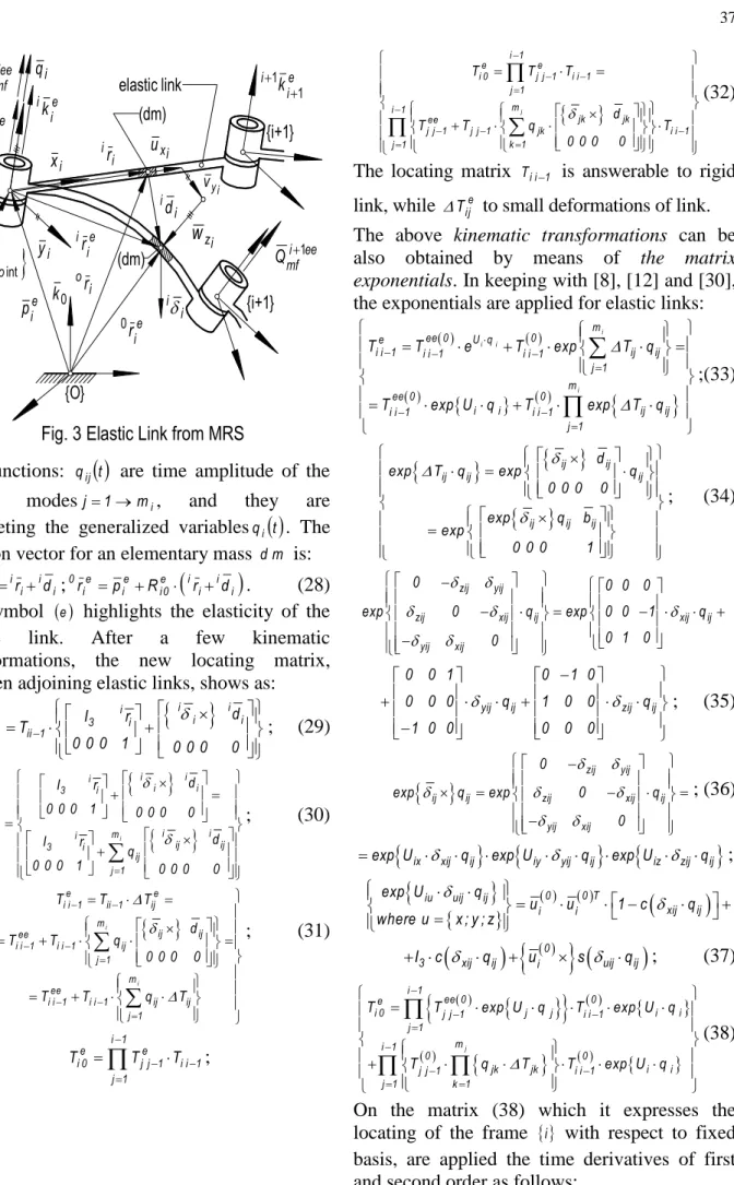
This section is devoted to define the generalized elastodynamics equations, when the robot links are dominated of flexibility properties. At first, a few kinematic transformations are described. In the aria of the small deflections, and considering the aspects from Fig.3, the time functions for the angular and linear deformations of the link i are written, according to [30] and [22] – [29] as follows:
zij yij ij x i
m 1 j
ij ij
i i m
1 j
ij i
z yi
i x i
i q t q t
(26)
ij ij ij i
m 1 j
ij ij
i i m
1 j
ij i
z yi i x i i
w v u t q d
t q w
v u
The functions: qij
t are time amplitude of the proper modesj1mi, and they arecompleting the generalized variablesqi
t . The position vector for an elementary mass dm is:i i i i e i
ir r d
;0rie pieRei0
iriidi
. (28) The symbol e highlights the elasticity of the kinetic link. After a few kinematic transformations, the new locating matrix, between adjoining elastic links, shows as:
i ii
i i
e 3 i
i i 1 ii 1
d
I r
T T
0 0 0 1 0 0 0 0
; (29)
i i i i i i 3 i eij m i i
i ij ij 3 i ij j 1 d I r
0 0 0 1 0 0 0 0
T
d
I r
q
0 0 0 1 0 0 0 0
; (30)
ii
e e
i i 1 ii 1 ij m
ij ij ee
i i 1 i i 1 ij j 1
m ee
i i 1 i i 1 ij ij j 1
T T T
d
T T q
0 0 0 0
T T q T
; (31)
i 1 e e i 0 j j 1 i i 1
j 1
T T T
;
j i 1 e ei 0 j j 1 i i 1 j 1
m i 1
jk jk ee
j j 1 j j 1 jk i i 1
k 1 j 1
T T T
d
T T q T
0 0 0 0
(32)The locating matrix Tii1 is answerable to rigid
link, while Tije to small deformations of link.
The above kinematic transformations can be also obtained by means of the matrix exponentials. In keeping with [8], [12] and [30], the exponentials are applied for elastic links:
i i i i m ee 0 U q 0e
i i 1 i i 1 i i 1 ij ij j 1 m
ee 0 0
i i ij ij i i 1 i i 1
j 1
T T e T exp T q
T exp U q T exp T q
;(33)
ij ijij ij ij
ij ij ij
d
exp T q exp q
0 0 0 0
exp q b
exp
0 0 0 1
; (34)
zij yij
zij xij ij xij ij yij xij
0 0 0 0
exp 0 q exp 0 0 1 q
0 1 0 0
yij ij zij ij
0 0 1 0 1 0
0 0 0 q 1 0 0 q
1 0 0 0 0 0
; (35)
ij ij zij zij yijxij ij yij xij0
exp q exp 0 q
0 ; (36)
ix xij ij
iy yij ij
iz zij ij
exp U q exp U q exp U q
;
0 0 T
iu uij ij
xij ij i i
exp U q
u u 1 c q
where u x ; y ; z
0
3 xij ij i uij ijI c q u s q
; (37)
j
i 1
ee 0 0
e
i 0 j j 1 j j i i 1 i i j 1
m i 1
0 0
jk jk i i j j 1 i i 1
j 1 k 1
T T exp U q T exp U q
T q T T exp U q
(38)On the matrix (38) which it expresses the locating of the frame i with respect to fixed basis, are applied the time derivatives of first and second order as follows:
{O} (dm) {i+1} elastic link {i} {i+1} (dm) i ir e i ir i id
e jo ik int
e i
p k0
e i r 0 i i e i i k 1 1 i x ee i mf
Q 1
iee mf
Q qi
e i ik iz w i y i y v i x u iee i Qö i or
;
(39)
; ;
(40)
; (41)
(42) In these expressions are substituted the matrices defined by means of the exponentials above shown. Considering (41) and (42), the angular rotation velocity and acceleration are defined as:
;
0 e
0 e 0 e 0 e T i ix iy izvect ;
;
. (43)
The linear velocity and acceleration of the elementary mass dm are defined by means of the time derivative applied on the position vector (3). As a result, the next expressions are:
0 e e e i i e i i i i0 i i i0 i
r p R r d R d ;
; (44)
(45)
Unlike MRS dominated of stiffness hypothesis, the column vector of the generalized variables, in the case of the structures with flexible links, is completed with (26) and (27) as below:
eT T
e
i ij
t t j 0 m i 1 n
; (46)
eT
i ij
ij t q t if j 0 ; q t if j 1
;
; ; (47)
;
; (48)
e 0 e i 0
e iv 0
j jk j
e i
0 J
J J m 1 k i 1 j
t q t q
J
. (49)
The above expression shows that every column of Jacobian matrix is function of generalized variables. Considering [8] and [30], its expression is defined by means of the classical transformations or matrix exponentials.
6. CONCLUSIONS
Within of this paper, the generalized elastokinematics equations have been analyzed for robot structures with flexible links. For define the kinematics and differential matrices functions in the case of the robot structures with rigid and elastic links have been applied the matrix exponentials, in accordance with the ME Algorithm. They are characterized through important advantages with respect to classical transformations. So, the matrix exponentials (ME) enjoy important advantages due to their compact form, easy geometric visualization and especially they avoid the frames typical to every kinetic link. As a result the matrix exponentials will stay at the basis of defining the linear and angular transfer matrices. By means of the matrix exponentials have been also determined all kinematic parameters. They characterize the equations of direct and control kinematics for any mechanical robot structure, regardless of its constructive complexity.
7. REFERENCES
[1] Appell, P., Sur une forme générale des equations de la dynamique, Paris, 1899
[2] Book, W. J., Recursive Lagrangian Dynamics
of Flexible Manipulator Arms, International Journal of Robotics Research, Vol. 3, 1984, pp.87-101.
[3] J.J. Craig, 2005, Introduction to Robotics: Mechanics and Control, 3rd edition, Pearson Prentice Hall, Upper Saddle River, NJ. [4]Fu K., Gonzales R., Lee C., Control, Sensing,
Vision and Intelligence, McGraw-Hill Book Co., International Edition, 1987
[5] Negrean I., Vușcan I., Haiduc N., Robotics. Kinematic and Dynamic Modeling, Editura Didactică și Pedagogică, R.A. București, 1998
[6] Negrean, I., Kinematics and Dynamics of Robots - Modelling•Experiment•Accuracy, Editura Didactica si Pedagogica R.A., ISBN 973-30-9313-0, Bucharest, Romania, 1999. [7] Negrean I., Mecanică avansată în Robotică,
ISBN 978-973-662-420-9, UT Press, Cluj-Napoca, Romania, 2008.
[8] Negrean, I., Negrean, D. C., Matrix
Exponentials to Robot Kinematics, 17th International Conference on CAD/CAM, Robotics and Factories of the Future, CARS&FOF 2001,Vol.2, pp. 1250-1257, Durban, South Africa, 2001.
[9] Negrean,I., Negrean, D.C., The Acceleration Energy to Robot Dynamics, Proceedings of A&QT-R (THETA 13) International Conference on Automation, Quality and Testing, Robotics, Tome II , pp. 59-64, Cluj-Napoca, Romania, 2002.
[10] Negrean, I., Negrean, D. C., Albeţel, D. G.,
An Approach of the Generalized Forces in the Robot Control, Proceedings, CSCS-14, 14th International Conference on Control Systems and Computer Science, Polytechnic University of Bucharest, Romania,
ISBN 973-8449-17-0, 2003, pp. 131-136. [11] Negrean, I., Pîslă, D., Negrean, D. C., New
Modeling with Matrix Exponentials in the Robot Accuracy, Proceedings, CSCS-14, 14th International Conference on control Systems and Computer Science, 2–5 July, 2003, Polytechnics University of Bucharest, ISBN 973-8449-17-0, pp. 143-148.
[12] Negrean, I., Albeţel, D. G., The Generalized Elastodynamics Equations in Robotics, Proceedings of AQTR 2004 IEEE-TTTC (THETA 14), International Conference on Automation, Quality and Testing, Robotics, Tome II, pp. 159-164, Cluj-Napoca, Romania, 2004.
[13] Negrean, I., Vușcan, I., New Formulations in the Applied Mechanics to Robotics,IEEE, International Conference on Automation, Quality and Testing, Robotics, pp. 284-289, Cluj-Napoca, Romania, 2006.
[14] Negrean, I., Energies of Acceleration in Advanced Robotics Dynamics, Applied Mechanics and Materials, ISSN: 1662-7482, vol 762, pp 67-73 Submitted: 2014-08-05 ©(2015)TransTech Publications Switzerland [15]Negrean I., New Formulations on
Acceleration Energy in Analytical Dynamics,
Applied Mechanics and Materials, vol. 823 pp 43-48 © (2016) TransTech Publications Switzerland Revised: 2015-09.
[16] Negrean I., New Formulations on Motion Equations in Analytical Dynamics, Applied Mechanics and Materials, vol. 823 (2016), pp 49-54 © (2016) TransTech Publications. [17] Negrean I., Advanced Notions in Analytical
Dynamics of Systems, Acta Technica Napocensis, Series: Applied Mathematics, Mechanics and Engineering, Vol. 60, Issue IV, November. 2017, pg. 491-502.
[18] Negrean I., Advanced Equations in Analytical Dynamics of Systems, Acta Technica Napocensis, Series: Applied Mathematics, Mechanics and Engineering, Vol. 60, Issue IV, November 2017, pg. 503-514.
[19] Negrean I., New Approaches on Notions from Advanced Mechanics, Acta Technica Napocensis, Series: Applied Mathematics, Mechanics and Engineering, Vol. 61, Issue II, June 2018, pg. 149-158.
[20] Negrean I., Generalized Forces in Analytical Dynamic of Systems, Acta Technica Napocensis, Series: Applied Mathematics, Mechanics and Engineering, Vol. 61, Issue II, June 2018, pg. 357-368. [21] Park, F.C., Computational Aspects of the
[22] Bratu, P., et all., The Dynamic Isolation Performances Analysis of The Vibrating Equipment with Elastic Links to a Fixed Base,
Acta Technica Napocensis, Series: Applied Mathematics, Mechanics and Engineering, Vol. 61, Issue I, March, pg. 23-28, 2018. [23] Mihălcică, M., Vlase, S., Identifiers for
Human Motion Analysis, Acta Technica Napocensis, Series: Applied Mathematics, Mechanics and Engineering, Vol. 60, Issue II, June, pg. 239-244, 2017.
[24] Vlase, S. Danasel, C. Scutaru, M. L. et al., Finite Element Analysis of a Two-Dimensional Linear Elastic Systems with a Plane "Rigid Motion". Romanian Journal of Physics, Vol. 59 (5-6), pp. 476-487, 2014. [25] Vlase, S., Dynamical Response of a
Multibody System with Flexible Elements
with a General Three-Dimensional
Motion. Romanian Journal of Physics, Vol. 57 (3-4),pp. 676-693, 2012.
[26] Vlase, S., Munteanu, M.V., Scutaru, M.L.,
On the Topological Description of the Multibody Systems. 19th International Symposium of the
Danube-Adria-Association-for-Automation-and-Manufacturing, Trnava, Slovakia, pp. 1493-1494, 2008.
[27] Vlase, S.; Teodorescu, P. P., Elasto-Dynamics of a Solid with A General "Rigid" Motion Using Fem Model Part I. Theoretical Approach. Romanian Journal of Physics, Vol.:58(7-8),pp. 872-881, 2013.
[28] Vlase, S., Itu, C., Structures with Symmetries Used in Civil Engineering, Acta Technica Napocensis, Series: Applied Mathematics, Mechanics and Engineering, Vol. 55, Issue III, pg. 689-692, 2012.
[29]Vlase, S., Năstac, C., Marin, M., Mihălcică, M., A Method for the Study of the Vibration of Mechanical Bars Systems with Symmetries,
Acta Technica Napocensis, Series: Applied Mathematics, Mechanics and Engineering, Vol. 60, Issue IV, pg. 539-544, 2017.
[30] Yuan, B.–S., Book, W. J., Huggins, J. D.,
Dynamics of Flexible Manipulator Arms: Alternative derivation, Verification, and Characteristics for Control, ASME Journal of Dynamics Systems, Measurements and Control, Vol. 115, 1993, pp.394-404.
Exponențiale de matrice în elastocinematica roboților
Rezumat: Obiectivul principal al lucrării constă în stabilirea ecuațiilor generalizate ale elastocinematicii structurilor de roboți cu elemente flexibile. Pentru cinematica și matricele diferențiale ale structurilor de robot cu elemente rigide și elastice se vor aplica exponențiale de matrice, în conformitate cu algoritmul dezvoltat de autorul principal. Ca urmare, exponențialele matrice vor sta la baza stabilirii matricelor de transfer liniare și unghiulare, determinându-se toți parametrii cinematici. În partea a doua a lucrării se va analiza structura elastocinematică a unui robot serial. Utilizând aceleași proprietăți ale exponențialelor de matrice, se vor stabili matricele de situare și derivatele în raport cu timpul corespunzătoare deformațiilor mici. Pe baza transformărilor diferențiale în partea finală a lucrării se vor determina vitezele și accelerațiile lineare și unghiulare, precum și matricea Jacobiană.
Iuliu NEGREAN Professor Ph.D., Member of the Academy of Technical Sciences of Romania, Director of Department of Mechanical Systems Engineering, Technical University of Cluj-Napoca, [email protected], http://users.utcluj.ro/~inegrean, Office Phone 0264/401616.