International Symposium on Information Theory and its Applications, ISITA2004 Parma, Italy, October 10–13, 2004
Decoder Implementation Issues for Low Density Parity Check Convolutional Codes
Andrew Schaefer
†, Arvind Sridharan
‡, Bernhard Koenig
†, Daniel J. Costello, Jr.
‡† Institute for Communications Engineering
Munich University of Technology email: [email protected]
‡ Department of Electrical Engineering
University of Notre Dame email: {asridhar,costello.2}@nd.edu
Abstract
1With the aim of implementing decoders for low density
parity check convolutional codes (LDPC-CC) in analog VLSI, we extend the investigations of [1].
We first provide further evidence of equivalent per-formance of digital and analog decoders by comparing probability density functions of output log-likelihood ratios and by examining the EXIT chart trajectories of each decoder type.
Next we make use of the fact that the shape of an analog decoding trajectory depends on the relative de-lays between processing elements in the decoder. These delays in turn are dependent on the circuit layout. By assuming a simple circuit layout model in which the total delay is constrained to be a constant, we de-termine the distribution of delays that results in the fastest decoder. We obtain initial ‘speed’ results from the EXIT charts, the accuracy of which we check with BER curves for particular signal to noise ratios (SNR) against simulation time. We finally provide two meth-ods for predicting trajectories for the analog decoders from the characteristic curves only, thus saving compu-tationally expensive simulations.
1. Introduction
In [2] an algebraic construction of LDPC-CC’s based on QC block codes was introduced. LDPC-CC’s have sparse factor graph representations, making BP decod-ing feasible: in fact, high memory LDPC-CC’s can be decoded in this fashion. Furthermore, LDPC-CC’s can be decoded by a BP based sliding window decoder that outputs decoding results continuously. With time-invariant LDPC-CC’s, the regular graph structure of the LDPC-CC’s can be exploited to implement decod-ing in analog usdecod-ing a simple rotatdecod-ing rdecod-ing architecture [1].
1This work was supported in part by NSF Grant
CCR02-05310, NASA Grant NAG5-12792 and the state of Indiana Sci-ence and Technology Fund.
Analog decoding involves the implementation of de-coding algorithms for channel codes in analog VLSI (for overviews see, e.g., [3][4][5]). The core idea is that the operations performed at the check and variable nodes of a belief propagation decoder can be implemented with simple transistor circuits. This differs from a conven-tional time discrete decoder in that messages are passed between nodes as time continuous signals, such that we can talk of ‘soft time’ decoding. Thus the analog de-coder attempts to solve the set of non-linear equations represented by the factor graph in continuous rather than discrete time. In the paper we will also use the term ‘time continuous decoder’ to refer to the analog decoder and the term ‘time discrete decoder’ to refer to the digital decoder.
After introducing some notation and terminology in section 2, section 3 compares the output probabil-ity densprobabil-ity functions (pdfs) of the log-likelihood ratios (L-values) of each decoder type. We make further com-parisons by examining decoder trajectories in section 4. In section 5 we show that circuit layout, which influ-ences the delays between the processing nodes of the decoder, has a significant effect on convergence speed. We use EXIT charts as well as BER curves as tools for determining convergence speed and also introduce methods for predicting analog decoding trajectories.
2. Definitions and Preliminaries
Let U ∈GF(2) with elements{+1,−1}, where +1 is the null element under⊕addition. The L-value (or LLR) of U is defined as L(U) = logP(U = +1) P(U =−1) and P(U =±1) = e±L(U) 1 +e±L(U), (1) whereP(U =u) denotes the probability that the ran-dom variableU takes on the valueu.
For descriptions of algebraically constructed LDPC-CCs, an introduction to the message passing algorithm used in decoders for these codes, and the fundamentals
!"# ! $# &' (
Figure 1: Structure of Rotating Ring Decoder. of analog decoding, we refer the reader to [1] and the references therein.
The proposed implementation idea for the analog rotating ring decoder is shown in figure 1. The de-coding of bits at time t is based only on the received L-values in the window from timet−Kto timet+K. In the rotating ring design, we rotate both the position where the decoded L-values are read out and the posi-tion where new received L-values are written into the ring at the transmission rate.
3. Decoder Output Distributions
For our analysis we considered a code of small mem-ory to reduce the complexity of testing (in an actual implementation we would use a code with much larger memory to take full advantage of the power of LDPC-CCs). Its parity check matrix is given by
H(D) = 1 D3 D1 D5 D2 D4 . (2)
Output L-value distributions for analog and digital rotating ring decoders at different values of the chan-nel SNR,Es/N0, are shown in figure 2. We see that in
all cases the L-value distributions show negligible dif-ferences. We have also performed tests for other codes which have given similar results. Finally, the results of [1], where we compared BERs, also imply that the tails of the pdfs are close to identical.
4. Convergence Points of Trajectories in EXIT Charts
Since the technique of EXIT charts is well estab-lished, we refer the reader to [6] for details. Briefly, based on the characteristic curves of component codes in a concatenated system, it is possible to predict it-erative decoding performance. We do this for
LDPC-−100 0 10 20 30 40 50 0.01 0.02 0.03 0.04 0.05 0.06 0.07 0.08
LLR L(z)
p(L(z))
digital analog−1dB
1dB
3dB
5dB
Figure 2: Probability distributions of output L-values.
L(z) is the output L-value andp(L(z)) is the pdf of the random variableL(z). VAR CHK R C R C L T VAR CHK L T z-1 z-1 IE,V IA,C IE,C IA,V IE,V IA,C IE,C IA,V
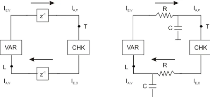
Figure 3: Schematic diagrams for the iterative decoders and points of measurements, L and T, for the extrinsic information on the EXIT charts.
CC’s by considering the set of variable nodes as one component decoder and the set of check nodes as the other. Referring to figure 3, we can model the time dis-crete decoder as having unit delay elements between the processing units (the mutual information I is la-belled with A and E for apriori and extrinsic, respec-tively, and C and V for check node and variable node, respectively). Likewise we model the time continuous decoder as having a simpleRC delay element between processing units. In each case, we can plot decoding trajectories by plotting the mutual information of ex-trinsic messages measured at points L and T on the figure at each time discrete step (for the time discrete decoder) or continuously (for the time continuous de-coder). In terms of the rotating ring design, we use only extrinsic messages close to the ’read out’ point of the decoder as our mutual information points. A trajectory is obtained by doing multiple decoder runs.
0 0.2 0.4 0.6 0.8 1 0 0.2 0.4 0.6 0.8 1 IA IB characteristic curves analog trajectories digital trajectories 2dB −4.1dB
Figure 4: Average trajectories for analog and digital decoders for Es/No of -4.1dB and 2dB. In each case both decoder trajectories reach the same point, as pre-dicted by the intersection of the characteristic curves.
Figure 4 shows two cases of channel SNR. We see that both types of decoders converge at the same points on the EXIT chart.
5. Using Circuit Layout to Enhance Analog De-coding Speed
We now wish to gain some insight into how circuit layout can affect the speed of analog decoding. We use a simplified model where we assume equal wire lengths for all connections from variable to check nodes and equal wire lengths for all connections from check to variable nodes (one can imagine that we set all lengths equal to the average wire length for that connection type). We further constrain the system such that the sum of this average wire length is constant. A justifica-tion for using this average model is that in the LDPC-CC, the connection lengths between variable and check nodes are limited to the code memory and cannot span the whole length of the code.
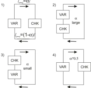
With reference to figure 5 (part 1), we set up the following problem: We are given a fixed wiring length
l that we arrange in the form of a square. The vari-able node and check node processing blocks may be placed anywhere on the square such that we assign a wire length lv→c = αl for the variable to check node connections and a wire lengthlc→v = (1−α)l for the check to variable node connections. We now ask which
α∈(0,1) results in the fastest decoding convergence? Parts 2), 3) and 4) of figure 5 show some example lay-outs for different values ofα.
VAR CHK VAR CHK VAR CHK VAR CHK a large a small a~0.5~ 1) 3) 2) 4)
l
v c=
a
l
l
c v=(1-
a)
l
Figure 5: Simplified circuit layout model 1), with ex-ample layouts for different values ofα, 2),3) and 4).
Note that in this experiment we are assuming the delay within the transistors themselves to be negligi-ble. This assumption is supported by the fact that the interconnect length is increasingly a dominant factor in circuit design [7]. If we were, however, to take this extra delay into account, it would mean only that we have a smaller available design range ofα.
Since the resistance and capacitance of a wire are both proportional to the length of the wire, if RC is the delay associated with the total length of wire, then
RCv→c =α2RC andRCc→v = (1−α)2RC.
Figure 6 shows how different EXIT trajectories are obtained for different values ofα. We see, for example, that forα= 0.1, the trajectory ’hugs’ the characteristic curve of the variable node. Later, in figures 11 and 12 we will plot the simulation time taken (as well as pre-dicted decoding time) to reach a point within a distance of 0.05 from the point (1,1) on the EXIT chart. We use this as an indication of convergence and hence decod-ing speed. We see that the decoddecod-ing speed is highest at
α= 0.5. For asymmetrical designs, a smallerαresults in a faster decoder than does a largerα. Tests at lower SNRs indicate similar results.
5.1. Confirmation of Results with BER Curves
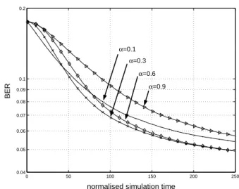
If the method of determining decoder speed with EXIT charts is to be useful, it should be verified also through BER measurements. Figure 7 shows the BER against simulation time at Es/N0 = 2dB for various
values of α. In figure 7 we see that after 250 time units we have the lowest BER for α = 0.3. Further
0 0.2 0.4 0.6 0.8 1 0 0.2 0.4 0.6 0.8 1 I A I B α = 0.1 α = 0.9 contours of equal elapsed time
characteristic curves
Figure 6: EXIT trajectories for different values of α
(dotted lines), points reached by different decoders at equal times (dashed lines), and bounds given by char-acteristic curves (outer solid lines). The top curve is forα= 0.1, the following curves are for increasingαin steps of 0.1.
emphasizing the need for proper circuit layout design, we see that the decoder with α= 0.3 reaches a BER of 10−4 about 1.5 times faster than the decoders with
α= 0.1 andα= 0.9.
The results compare reasonably well with those of the EXIT charts, although the EXIT charts indicate that the decoder withα= 0.5 is slightly faster than the decoder with α= 0.3 (this small difference compared to the BER results may be due to the definition of convergence assumed for the EXIT charts).
To check that other SNR values do not have other optimal α, we performed an additional BER test at
Es/N0 = −2.8dB, the results of which are shown in
figure 8. Again we find a similar behaviour with respect toαand that a choice ofα= 0.3 results in the fastest decoder (at a target BER of 0.06, this decoder is more than 1.5 times faster than the decoder havingα= 0.9).
5.2. Prediction of Analog EXIT Trajectories
We now investigate two techniques for predicting analog decoding trajectories. Note that in a time dis-crete decoder, trajectory prediction means simply draw-ing a step function between the two characteristic curves. In the time continuous domain, this task is more de-manding.
The first technique (which we will refer to as method A), involves working with mutual information values
0 50 100 150 200 250
10−4 10−3 10−2
BER
normalised simulation time
α=0.1
α=0.3
α=0.6
α=0.9
Figure 7: BER at Es/No = 2dB as a function of de-coding time for circuit layouts with varying values of
α. 0 50 100 150 200 250 0.04 0.05 0.06 0.07 0.08 0.09 0.1 0.2 BER
normalised simulation time
α=0.1
α=0.3
α=0.6
α=0.9
Figure 8: BER at Es/No = −2.8dB as a function of decoding time for circuit layouts with varying values of
α.
only. We view the decoder as only processing mutual information values, which are also exchanged between decoders through the RC delay elements. We now for-malize the description.
For the component decoders (which we label now as 1 and 2) in a concatenation, we haveIE1 =f1(IA1) and
IE2 =f2(IA2). Given the functionsf1(.) andf2(.), the
evolution of the mutual informations in the discrete timealgorithm can bepredicted by the equations
IE1,k+1=f1(IA1,k) and IE2,k+2 =f2(IA2,k+1). (3)
problem such that we are effectively looking for theIE1 that satisfies,
IE1 =f2(f1(IE1)). (4) How we solve for the fixed point of equation (4) is our choice. One possibility is to use the method of successive substitution by applying the equations of (3). We may also introduce step sizesh1 and h2 into
(3) to obtain,
IE1,k+1 = (1−h1)·IE1,k+h1·f1(IA1,k),
IE2,k+1 = (1−h2)·IE2,k+h2·f2(IA2,k), (5) where the equations now run in parallel and IA1,k =
IE2,k and IA2,k =IE1,k. Note again that we are oper-ating directly on mutual information values.
Now, we allowh1andh2 to tend to zero (and here
we emphasize that the delays need not be uniform) to obtain the time continuous equations,
τ1dIE1
dt = f1(IA1)−IE1,
τ2
dIE2
dt = f2(IA2)−IE2 (6)
whereτ1andτ2 represent delay constants.
Examining (6), and with IA1,k=IE2,k andIA2,k=
IE1,k, we see that if dIE 1 dt = 0 and dIE 1 dt = 0 (i.e., the algorithm converges), then we have the same equation as (4).
In the second technique (which we will refer to as method B), we no longer pass mutual information val-ues through RC delay elements. Instead, the mutual information values are first converted to equivalent L-value means. These L-values are then passed through the RC delay elements and at the output they are converted to mutual information values again.
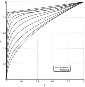
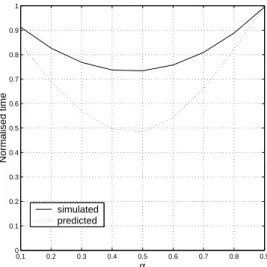
Results are shown in figures 9 and 10. We see that for both prediction methods, the trajectories match reasonably well. Figures 11 and 12 show the predic-tion of decoder speed against the actual decoder speed as measured using the EXIT chart. Here we note that, although the predictions are not exact, they show the same tendencies. Method A predicts that the fastest decoder has α = 0.5 and that this decoder requires half as much time as the slowest decoder to converge. Method B predicts the fastest decoder has α = 0.4 and that this decoder requires 3/4 as much time as the slowest decoder to converge (the simulated EXIT chart results show that α = 0.5 gives the fastest decoder). Also of note in these figures is that prediction method B approximates the convergence time more accurately than method A. 0 0.2 0.4 0.6 0.8 1 0 0.2 0.4 0.6 0.8 1 I L I T simulated predicted
Figure 9: Simulated (solid line) and predicted (dashed line, prediction method A) decoding trajectories for analog decoders having varying values of α. Results are forEs/N0= 2dB. 0 0.2 0.4 0.6 0.8 1 0 0.2 0.4 0.6 0.8 1 I L I T simulated predicted
Figure 10: Simulated (solid line) and predicted (dashed line, prediction method B) decoding trajectories for analog decoders having varying values of α. Results are forEs/N0= 2dB.
6. Conclusions
We have extended the results of [1] and further demonstrated that analog implementations of LDPC-CC decoders produce equivalent results to their digi-tal counterparts by comparing the probability distribu-tions of the decoder output reliabilities. Additionally,
0.1 0.2 0.3 0.4 0.5 0.6 0.7 0.8 0.9 0 0.1 0.2 0.3 0.4 0.5 0.6 0.7 0.8 0.9 1 Normalised time α simulated predicted
Figure 11: Simulated (solid line) and predicted (dashed line) convergence times (prediction method A). Time is normalized such that the slowest decoder in each case, corresponding toα= 0.9, has the same speed. Results are forEs/N0= 2dB.
we have seen that, given a certain SNR, both digital and analog decoders converge to the same point on the EXIT chart as predicted by the characteristic curves of the variable and check nodes.
We then considered the effect of circuit layout on analog decoder speed, assuming a fixed wire length for interconnects which could be assigned freely between the check to variable connecting wires and the vari-able to check connecting wires. This simple experiment demonstrates that circuit layout can have a significant effect on decoder speed (up to a factor of approximately 1.5 as measured using a target BER). In particular, it is unwise to allow a large delay for the variable to check node connection.
The same principle can be applied to all types of analog decoders for concatenated codes. A general rule seems to be to try and keep the delays between compo-nent decoders approximately the same. This depends, however, on the degree of asymmetry between the de-coder characteristic curves. We see that EXIT chart trajectories give a good indication of decoder speed for various values of α. Finally, note that we have used a relatively simple delay model for this concatenated code, and it is certainly possible to construct more com-plicated models that are closer to actual circuit layout designs.
References
[1] A. Schaefer, A. Sridharan, M. Moerz, J. Hage-nauer, D.J. Costello, ”Analog Rotating Ring
De-0.1 0.2 0.3 0.4 0.5 0.6 0.7 0.8 0.9 0 0.1 0.2 0.3 0.4 0.5 0.6 0.7 0.8 0.9 1 Normalised time α simulated predicted
Figure 12: Same results as in figure 11 but for predic-tion method B.
coder for an LDPC Convolutional Code”, inProc. Inf. Theory Workshop, Paris, France, April 2003, p. 226-229
[2] A. Sridharan, D.J. Costello, D. Sridhara, T. Fuja, R.M. Tanner, “A Construction for Low Den-sity Parity Check Convolutional Codes Based on Quasi-Cyclic Block Codes”, inProc of IEEE Int. Symp. on Inf. Theory, Lausanne, Switzerland, July 2002, p. 481.
[3] H.-A. Loeliger, F. Lustenberger, M. Helfenstein, F. Tark¨oy, “Probability and Propagation in Ana-log VLSI”, inIEEE Transactions on Information Theory, vol. 47, pp. 837-843, Feb. 2001.
[4] C. Winstead, J. Dai, S. Yu, R. Harrison, C. Myers, C. Schlegel, “Analog Decoding of Product Codes”, in Proc. of Int. Symp. on Inf. Theory, Lausanne, Switzerland, July 2002, p. 230.
[5] J. Hagenauer, M. Moerz, A. Schaefer, “ Analog Decoders and Receivers for High Speed Applica-tions”, inProc. of 2002 Int. Zurich Sem. on Broad-band Comm., Zurich, Switzerland, Feb. 2002, pp. 3.1-3.8.
[6] S. ten Brink, “Convergence behavior of iteratively decoded parallel concatenated codes,” in IEEE Transactions on Communications, vol. 49, pp. 1727–1736, Oct. 2001.
[7] D. Mlyinek, Y. Leblebici, ”Design of VLSI Sys-tems”, http://vlsi.wpi.edu/webcourse, chapter 4.