XA PIPING BENCHMARK PROBLEMS

3.2 PIPING BENCHMARK PROBLEMS COMPUTER ANALYSIS WITH THE CEASEMT FINITE

ELEMENT SYSTEM by

H. Bung, G. Clement, A. Hoffmann and H. Jakubowicz

This section presents results for the analyses of all three International Piping Benchmark Problems. An inelastic analysis of each problem was performed using a full three-dimensional shell analysis (TRICO code) and a simplified piping analysis based on beam theory

PIPING BENCHMARK PROBLEMS

COMPUTER ANALYSIS WITH THE CEASEMT FINITE ELEMENT SYSTEM

H. BUNG, G..CLEMENT, A. HOFFMANN, H. JAKUBOWICZ

Les informations contenues dans ce document sont reservees aux destir.ataires noramement designes. Elles ne peuvent

recevoir aucune autre diffusion sans 1'autorisation expresse du Departement des Etudes Mecaniques et Thermiques.

FOREWORD

In accordance with recommandations, at the 1976 IWGFR specialists1 Meeting on High-Temperature Structural Design, three experimental benchmark piping problems were selected. The D.E.M.T (Departement des Etudes Mecaniques et Thermiques) of the French Atomic Energy Commission has contributed to this benchmark effort by computing the three proposed problems.

Two different types of analyses were conducted for each problem. Firstly a full three dimensional shell analysis was performed then a simplified piping analysis method is used. The comparison of these twc analyses 'with the experimental results and between themselves permits not only to assess non linear finite element analysis for piping but also the advan-tages and limitations of simplified methods.

This report is divided in three parts. The first part presents the three dimensional analyses for the benchmark problems. The second part presents the simplified piping ana-lysis of the same problems. The third part is devoted to the comparaison between the two analysises.

The first and second parts present the respectively used computer codes and a brief summary of the theories used in them. Special mention is made of the global method and of the e Hoffmann method for non linear analysis. The elbow element of the simplified method is described. Input and output of both codes are presented. Then the three benchmark problems are described with all relevant data for the computation. The finite element idealisation is given and the results are shown on

tables and diagrams. The computed results are compared to the measured results.

The third part presents the hypotheses made to explain the observed differences between the three dimensional computa-tion and the measured data. Then are explained the differences

between the two types of analyses. All these explanations are supported by further computations with different shapes, mate-rial data or thicknesses. A cost effectiveness analysis is made for the two types of analysis methods.

CONTENTS

Pages FOREWORD. 0 . 1 PART ONE - PIPING BENCHMARK PROBLEMS ANALYSIS WITH THE THREE DIMEN-SIONAL SHELL ANALYSIS COMPUTER CODE TRICO.

1.- A three dimensional e l a s t i c - p l a s t i c - c r e e p s h e l l analysis program.

1 . 1 . - Introduction. l.l 1.2.- Description of the code TRICO. 1.1 1 . 2 . 1 . - General f e a t u r e s . 1.1 1 . 2 . 2 . - The global method. 1.2 1 . 2 . 3 . - The £*-Hoffmann method 1.5 1.2.4.- Material data input. 1.15 1 . 2 . 5 . - Input and output of TRICO. 1.17 1.3.- Elbow-pipe assembly subjected to in-plane moment 1.17 loading a t 593° C. 1 . 3 . 1 . - Problem d e s c r i p t i o n . 1.17 1 . 3 . 2 . - The f i n i t e element i d e a l i s a t i o n . 1.20 1 . 3 . 3 . - Results. 1.22 1.3.4.- Conclusions. 1.25 1.4.- Elevated temperature e l a s t i c - p l a s t i c - c r e e p t e s t of an elbow subjected to in plane moment loading. 1.51

1 . 4 . 1 . - Problem d e s c r i p t i o n . 1.5! 1 . 4 . 2 . - The f i n i t e element i d e a l i s a t i o n 1.53 1 . 4 . 3 . - Results. 1.55 1.4.4.- Conclusions. 1.55 1.5.- Room-temperature e l a s t i c - p l a s t i c response of a thin walled elbow subjected t o in plane bending loads. 1-69

1 . 5 . 1 . - Problem d e s c r i p t i o n . '-69 1. 5. 2. - The finite element idealisation 1.70 1. 5. 3. - Description of the implementation of large

displacements in the £ -Hoffmann method for non linear

structural analysis 1.73 1.5.4. - Results 1.76

PART TWO - PIPING BENCHMARK PROBLEMS ANALYSIS WITH A SIMPLIFIED PIPING ANALYSIS METHOD.

2.- A simplified method for non linear piping analysis.

2.1.- Introduction. 2.1 2.2.- Description of the simplified piping analysis

computer code TEDEL. 2.1 2.2.1.- General features. 2.1 2.2.2.- The global method applied to pipes. 2.2 2.2.3.- The elbow element. 2.5 2.2.4.- Other features. 2.8 2.2.5.- Input and output of the TEDEL computer code. 2.8 2.3.- Elbow-pipe assembly subjected to in-plane moment

loading at 593° C. 2.11 2.3.1.- The finite element idealisation. 2.11 2.3.2.- Results. 2.13 2.3.3.- Conclusions. 2.17 2.4.- Elevated temperature elastic-plastic-creep test of an elbow subjected to in-plane moment loading. 2.43

2.4.1.- The finite element idealisation. 2.43 2.4.2.- Results. 2.45

2.5.- Room-temperature elastic-plastic response of a

thin walled elbow subjected to in plane bending loads. 2.52 2.5.1.- The finite element idealisation. 2.52 2.5.2.- Results. 2.55 2.5.3.- Conclusions. 2.56

PART THREE - ANALYSIS OF BENCHMARK TESTS AND COMPUTER RESULTS. 3.- Evaluation of the benchmark problems. 3.1

3.1.- Introduction. 3.1 3.2.- Influence of material data. 3.2

3.3 - Influence of straight parts on elbows. 3.7

3.4 - Influence of geometrical data. 3.11

3.5 - Cost effectiveness. 3.17

3.6 - Closure. 3.19

PART ONE

PIPING BENCHMARK PROBLEMS ANALYSIS WITH THE THREE DIMENSIONAL SHELL ANALYSIS

COMPUTER CODE TRICO

1 A THREE DIMENSIONAL ELASTIC-PLASTIC-CREEP SHELL ANALYSIS PROGRAM

1.1 Introduction

The TRICO shell analysis computer code is part of the CEASEMT finite element system. It has access to all of this system capabilities. This system is caracterised by a modular architecture especially designed for non linear and dynamic structural problems. A complete library of elements is available as well as a huge capability of pre and post-processors for two and three dimensional problems.

The COCO pre-processor {reference 3) is a mesh generator with its own geometrically oriented language. The TEMPS and ESPACE post-processors (reference 4) are used to display graphically all relevant results respectively in time for a given point and in space for a given time.

1.2 Description of the code TRICO {references 1, 2)

1.2.1 General features

As raost of the CEASEMT system programs the TRICO program is based on the finite element method. The TRICO program uses a flat three nodes triangulare constant stress element. Each node has six degrees of freedom. A truss element is also included and can be used in connection with the plate element.

The TRICO program can solve static or dynamic problems. It can search for eigenvalues or give the response to any

excitation or to a varying load by time step integration. It can solve Elastic-plastic-creep analysis with large displace-ments as well as problems in thermoplasticity.

Due to its dynamic storage allocation capability, the TRICO program can solve problems with a large number of unknows. Its limits being those of the out of core storage of the computer center.

The loading conditions and boundary conditions are numerous and general enough for all engineering needs. It is possible to apply concentrated or distributed forces and

moments as well as pressure, dead weight or thermal loads. The displacements can be imposed in any direction. Relations between displacements or between forces and displacements are easily taken in account as well as the symetry conditions.

1.2.2 The global method (Ref.9)

The basis of this formalism is the notion of genera-lised stresses and strains introduced by Prager (reference 18). These generalised stresses and strains are placed in duality by a bilinear form expressing the virtual work. The equations of plasticity are then expressed directly in terms of these generalised stresses and strains.

For the plate (or shell) element the generalised stresses are the membrane tensions (N., No, N O and the bending moments (M,, V\.~, M J . Corresponding to these stresses are the generalised strains defined by membrane strains (e., e_, e.)

and curvature variations (x-,, x^/ x3) •

To define a generalised yield surface the second order invariants of the generalised stresses deviator are used in conjonction with the Von Mises criterion. The three invariants are

N2 M2 MN = Nx 2 = M l 2 cosQ =

and the yield surface is an expression of the form

P(M,N/cos0,u1,u2/«--) = °

where vu, y2, ... are material history parameters.

Hill's principle for plastic flow applied to these relations produces the following relations

dex dX dX de3 3E 3N 3F 3N 3F N N 3 -0 N

2-°

N .bNo 1 + — -1 N 1 N 3F i £ 3cosQ 3F 3cos0 3M, M.-0.5M, ± £ M M2- O . 5M l M 3N N N 3cos9 M 3F M,-0.5M2 1 3F N1~0.5N2 dX dx2 dX dx3 dX 3M 3F 3M 3F 3M M2 3M M M -0. M 3 | 1 M M 3cos0 1 ? F N M 3 cos's 3F 3N3 3cos0 N N

2-°-

5N

l

N

As usually dX is obtained by identifying the relation between equivalent generalised stress and strain intensities to the tensile curve.

In practice in the computer program these generalised stresses and strains are normalised to stress and strain quan-tities by taking in account the thickness of the plate or the shell.

The hardening law can be either one of the following rules : isotropic hardening, kinematic hardening or a multi-layer model.

Then the usual initial stress method, with some

improvements described below, is applied to solve by increments and iterations these non linear equations. For a load increment AF the static equilibrium equation must obviously be satisfied.

This is accom-plished by the so called "external iterations". If the associated stress distribution does violate the yield criteria in some part of the structure, the stress must be brought back on the stress-strain curve by allowing plastic flow in that part. This is accomplished by the so called "internal iterations".

To be more specific let AF be the load increment and AU the displacement increment. Then [ K J {AU} = {AF} where^V) is the stiffness matrix. If the yield criterion is violated the internal iterations will produce a plastic flow increment

Aep. To satisfie equilibrium a load increment

I

=

£ '

v m CBm] T [DmI1

-

i

-is computed where {em} = C ^ l {°} '• {°m} = C^iiO {zm) r m -is an element number and Vrn. the volume of the element. And then an external iteration is performed that is to say the

[K] {AU}2 = {AR} + {AFP11

The yield criterion is then verified again and so on. The iterations are stopped when {AFP} = {AFP} or if they differ only by a small amount.

1.2.3 The e*-Hoffmann method

At an equilibrium position the equation

[ B ] T {aQ} = {FQ} (1)

is verified. Let {dF} be an infinitesimal increment of load then

[ B ] T {a} = {FQ} + {dF} (2) if {cr} = {aQ} + {da} then it can be deduced that

[ B ] T {da} = { d F } (3) But {da} = [ D ] {dee}= [ D ] ({det} - {dep}) (4)

and {det} = [ B 3 {du} (5)

where ee, e , ep are the elastic, total and plastic strains an u the displacement. Finally the incremental equilibrium equation can be written as

[iff {du} = [ B ] T [ D ] [ B ] {du}={dF} + [B] T [ D ] {dep} (6)

The Prandtl-Reuss equation for the Von Mises yield criteria can be written as

{dep} = [ M ] ±2i d e * (7) a

CM]'

=

2

0

0

thus equations (4) and (7) produces

{da} = C

D

3 {de

1

} - M W ^-

de

*

ax

and dividing by de a fondamental equation is obtained

<H*>

-

M

(8)

(9)

with [Vj = [ D ] [ M ] and {do

1

} = [D] {d£

fc

} .

This differential equation is valid only if de 5^ 0. To summarise the previous discussion the following two equations must be integrated in order to solve the plasticity problem :

if a*({a} + {da}) < f(£*) then de* = 0 and {da} = {dat}=[A] {du}

if o*\{o} + {da}) > f(e*) then de > 0 and { — J } = {S 2J } - [ A ]

wheref is the yield surface.

For a finite increment of load {DR} the first external iteration produces the first displacement by

[ ] X = {AR} (10)

and the stress increment is known by

{Ao*} = [A] { A U )3 (11)

If a* ({ao> + {Aa*}) < f(e*Q) then Ae* = 0

and {Aa} = {Aat}.

But if a* ({ao> + {Aafc}) > f(e*Q)then Ae* > 0 and {Acr} is given by the relation

a* ({aQ} + {Aa}) = f(e*o + Ae*)

which says only that the stress is on the tensile curve at the end of the load step.

The problem now is how to integrate the differential stress equation between e and e + Ae with

. e equivalent strain at the beginning of the load step

. £ *+ Ae* equivalent strain at the end of the load step

. {a } stress at the beginning of the load step

• {a } + {Aa} stress at the end of the load step

1.2.3.1 The fondamental hypothesis

The value of {—j} is not known so it will be supposed o*

}This consists

*

{ j

to be constant on the e Ceo*' e * + A e -I interval and equal to {——-}. This consists only to assume that the stress

Ae*

To solve the differential system t da de Aa } " (12) Ae

a diagonalisation is performed on the A matrix whose eigenvalues are X = 0 and X_ = X- = X. =

ding eigenvectors are

= j. The correspon-Vl " 1/VS 1/V3 l/VT 0 0 0 V2 = 1/V5" -1/V2 0 0 0 0 V3 = 1/VS" 1/V^ -2/V6 0 0 0 V4 " 0 0 0 1 0 0 V5 = 0 0 0 0 1 0 V6 = 0 0 0 0 0 1

In this base the {a} vector has a. components and

{a} Z a. {v.}

thus the differential system can be written da. Aa.t a.

d£ As

—

a* (13)

these equations are uncoupled and can be solved separately. The equations are analyticaly integrated and the solutions included in the computer program. Two cases will be developped perfec plastic material and hardening material.

1.2.3.2 Perfect plastic material

The solutions of the differential equations are * t

a. (e*) = C exp( £ — ) + — £— (14)

i Ae the C constant being given by the relation

ai( £o

cr^ is the stress value at the beginning of the load step expressed in the base {vi> of eigenvectors of [ V ] - Then

Aa.t i X.i k A ait Xi A e * _!L _ i _} e x p (_ i u (15)

at the end of the load step (in fact at e * + A e * ) , where {Aa } = Z A ai t { v±} .

The only unknow in the last equation is Ae*. Its ietermined by writti

stress-strain curve. That is _*

value is determined by writting than the stresses o. are on the

({a±}) = k ₍₁₆₎

The Newton-Raphson iterative method is used to solve this non linear equation in Ae*. Only a few iterations (2 or 3) are necessary. This method is shown schematically on figure

1.2.3. ^ ^

1.2.3.3 Hardening material (isotropic case)

In this case a is not any nore a constant in equation (13). In the Zeo*t e o* + A e* D interval o* does increase and

this variation is accounted for approximatively.

A limited expansion to the first order, in Ae , of equation (15) and of the tensile curse is made and this leads to a± Aal Ae 0 ( A E*? ) (17) and a* = aQ* + h A E * ,dc (18) * where h = (—r-) . is the tangent to the tensile curve at e

o

This set of equations (17 and 18) is solved in Ae and a point (a. , Ae() is obtained as shown on figure 1.2.4.

Fig 1.2.4 - Solution of equations 17 and 18.

The internal iterations are carried on now on equations (15) and (16) as in the perfect plasticity case but with the mean valve <J = k = jio + a ) for the load step. This choice does verify the flow equations only in average on the load step but the error which is introduced is very low.

At the end of the internal iterations the stresses are given by {a } + {Aa} and they are on the stress-strain curve. The new value e + Ae is known as well as the plastic defor-mation variation.

{Aep} = [ D ] -1 ({Aafc} - {Aa})

The plastic load {AFP} necessary to reeguilibrate the structure is then given by

{ A FP} = i / CBm: T H A O J O - Ucm}) dvm

m vm

This force is added to the second member of the equi-librium equation

0 0 {AU> = {AR} + {AFP}

which is solved by external iterations.

1.2.3.4 Convergence criteria.An acceleration method

The external iterations are stopped when {AFP} does not change any more. That is done in the computer program by the following criteria. Let a be the value of a (a + Aa - Aa p)

ij. j . " i . p o n n

and a . the value of a (a + Aa - Aa , ) . Then these n~i o n n— i.

iterations are stopped when

Pn "• ^ ^" max an

for all the elements and where p is the convergence criteria supplied by the user.

The same method applies to the internal iterations but with p /^ as convergence criteria.

Depending on material caracteristics this convergence can be slow. An acceleration method based on the following extrapolation method was then included in the program.

Let Ae be the variation of equivalent plastic

deformation obtained at the issue of the n external interation the associat

is defined by

and the associated internal iterations. The rate of convergence xn

T

n n—1 A en - 1 ~ A en-2

This rate is suppose to stabilise after only a few iterations. At the user's demand every m iterations the limit of the Ae n sequence is then calculated by

A * A *

A em-1 " A em-2 and

Ae* = ^ L (Ae *

-which is the limit of the geometric sequence. Then the plastic deformations are modified in the same proportions

{ A e

P) =

^ 1

n

(The upper index p is for plastic) and the corresponding plastics loads ^ are used for the following external iterations.

For some problems if this extrapolation method fails every few iterations the tangential stiffness matrix can be cal-culated at the users demand.

1.2.3.4 Hardening material (Kinematic hardening)

The yield criteria is written F({a-«}) = 0 and the stress-strain curve supposed to be bilinear. The Prager-Ziegler hypothesis is used to determine the hardening parameter {q}.

{do} = du ({a -a})

dp is obtained by differentiating the yield surface equation and using the plastic flow equations. That is

= de*p 3f 9{a-ct} ({c-a}) and {- df a* = f({a-a}) d f({a-a}) = 0 => 1 {da} = f df ld{a-nJ T = 0 {(a-a)} dy Then

But for constant a

and

dy = da* = h de*P

where h is the derivative of the tensile curve at eQ . This modifies the algorithm previously described in the following manner

{da} = {da

t

}

-

[M]

— — {a

-

a}

0

{da}n = -4- de*P {a - a},

{d(a-a)}1 = {dat}1 - C M ] + h [l]){o-a)1 de* P

where £l] is the unit matrix. It is seen that this equation is the equation (8) by changing {o-a} to {a}. The same integration method can then be applied. This method gives simultanously the solutions of the equation of plasticity and the displacements of the yield surface defined by {da}.

1.2.3.5 Application to creep problems

As usually the first step is to write the equation of equilibrium

C B ] {a} = {F} (1)

and the equation for the stresses

{a} = {aQ} + [ D ] ({Aet} - {AeF}) (2)

The creep flow is given by the following equation

on the time interval Cfco' tQ + At].

Equations (1) and (2) are combined and as above it is obtained

= {AF} + M [D] { A£P }Q + [ B ] [D] {A£P}

and the same iterative method is applied. The question here is how do one obtain {&e } from (3). The integration is nume-rically conducted with the simple equation

and {Aep} is then put in equation (4). This last equation replaces the internal iterations previously defined. After equilibrium is obtained at the n^1 iterate it is necessary to verify that the stress at the end of the time step is the stress which was used to determine {Ae^1}. If it is not the case a new iteration is performed.

1.2.4 Material data input

For plastic or creep analyses the ability to intro-duce easily material datas in various manners is very important. Generaly these data are given point by point, sometimes an

analytical curve- is assumed and they are also cases where it is necessary to smooth and fit the datas by numerical means. In the TRICO program the stress-strain curves are supplied by either two ways : point by point with the other clatar related to the problem or by a user supplied subroutine where any type of constitutive equation can be accounted for. The point by

point data are used by TRICO in conjonction with a quadratic inter-polation. The creep data a*"e always given by the user supplied subroutine in the form of the function.

•* * *

e = 0 <e , a , t, T, ..., ...)

where e is the strain intensity, a the stress intensity, t the time, T the temperature etc ... Any argument of this function can be omitted and other arguments can be added. If the creep data are given point by point the user supplied subroutine must be provided with an interpolation scheme. This way of dealing with creep leaves the designer free to choose any hardening rule

1.2.5 Input and output of TRICO

The input must always begin with some parameters on the number of nodes and elements and other values, to allocate the computer memory necessary for the problem. All the other data are input in free format fields in any order due to the use of code names to specify the different data categories. The input is generaly composed by

- The mesh : coordinates of the points, numbers defining the elements

- The thicknesses of the elements

- Some material properties :

. Young modulus . Poisson's ratio

. Stress-strain curves {if given point by point)

- The loads

- The load and time increments

- The boundary conditions

- Parameters for non linear analysis : maximal number of itera-tions , convergence criteria

- Parameters for selection of the printed output.

The results are listed or stored on computer files for latter retrieval by post-processor codes. They can be visua-lized on graphic display units, hard copy or plotters.

These post-processor codes can be used either by the batch processing mode or the interactive time sharing mode.

All input data are printed. Then for each time or load steps the following results are printed :

- number of plastic elements,actual convergence error, maximal stress and strain intensities. Actual loads and time incre-ments. Number of iterations.

- At selected elements : the principal strains and curvature variations.

For selected time or load steps the following results are printed

- The displacements and rotations

- The boundary reactions

-• The principal stresses and moments

1 3 Elbow-Pipe Assembly Subjected to&In-Plane Moment Loading at S93°C

1.3.1 Problem description (ref. 6)

1.3.1.1 Geometry

The Elbow-pipe Assembly tested at Battelle-Columbus Laboratories is a 101.6 mm sched-10 90° elbow with a 152.4 mm bend radius welded to two 324 mm lenghts of sched - 10 pipes.

(Fig. 1.3.1) . The elbow wall thicknesses and diameter were measured at selected grid points (table 1.3.1 and Fig. 1.3.2) .

a 0° 22.5° 45° 67.5° 90° Wall thicknesses in mm <j>=0° 3.02 2.74 2.76 3.37 2.79 90° 3.2 2.84 2.54 2.81 3.07 180° 3.12 2.94 2.94 2.99 3.12 270° 2.97 3.40 3.50 3.40 3.02 Outside diameter 0° to 180° 114.25 114.50 114.78 115 115.34 90° to 270° 114.88 114.75 114 114.22 113.66

Table 1.3.1 - Dimensions of elbow

The average wall thickness is 3 mm and average outside diameter is 114.53 mm. The pipe legs have a wall thickness of 3.07 + 0.05 mm, an outside diameter of 114.25 + 0.25 mm and a length of 323.85 mm.

A rigid frame shown on fig. 3.1 is used to apply the loads.

1.3.1.2 Loads and boundary conditions

As system of dead weights was used to load the assembly. These loads produce a constant moment in the assem-bly. On figure 1.3.3 the loads are noted as Fj^ and F2 > The load histogram is shown on figure 1.3.4. A first load of 1382 N is applied on each loading point producing a bending moment of 843 Nm. The specimen is held at this load for 295 hours. The load is then increased to 1827 N producing a bending moment of 1114 Nm. This load is held for another 44 hours. At this time the test is ended. The temperature during all the test is maintained at 593°C + 5.6°C.

The Elbow pipe assembly is rigidly fastened at the other end.

1.3.1.3 Material

The elbow and pipe legs are made of type 304 stainless steel. The material properties are given in reference 5.

Young modulus 149 652 N/iran

Poisson's ratio 0.3

The stress-strain curve at 593°C is given by the following formula

ep = 4.59 x 1 0 "4 1 a9'3 3 7 7

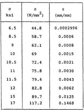
where a is in psi and £„ the plastic strain is in/in. The tensile curve values are given below in table 1.3.2 and the correspon-ding graphe is shown on fig. 1.3.5.

a ksi 6.5 8.5 9 10 10.5 11 11.5 12 15 17 a (N/mm2) 44.8 58.7 62.1 69 72.4 75.8 79.4 82.8 89.7 117.2 e (mm/mm) 0.0002996 0.0006 0.0008 0.0015 0.0021 0.0030 0.0043 0.0062 0.0125 0.1468

The creep data are given by the reference 5 table 2.

1.3.2 The finite element idealisation

1.3.2.1 Geometry

Half of the elbow pipe assembly due to symmetry

conditions) is meshed with 770 triangular elements and 432 nodes. The mesh, the element numbering and nodal numbering are

presented on figures 1.3.6, 1.3.7 and 1.3.8.

Each element is given its appropriate thickness. The eguithickness^ lines are represented on figure 1.3.9.

The frame at the free end was not meshed but repre-sented by a rigid flange. This flange is reprerepre-sented in the mesh by the last row of elements (749 to 770) which were given a 45 mm thickness.

1.3.2.2 Loads and boundary conditions

The forces are introduced directly on the mesh on points number 421 and 432. They are given a value taking in account the effect of the beams length. That is

F

F * x R = — x 304.8 mm 1 2

where R is the mean radius of the pipe, and, due to the symmetry condition, only half of the load is applied.

* _ 1382 x 304.8 _ , _, _-Fl " 2 x 55.63 " 3 7 8 6-0 3 N The same value is given to F» .

By the same formula the second load is obtained as 5005.12N.

The boundary conditions as mentionned previously are symmetry conditions for the XOY plane and of the clamped type conditions for the fixed pipe end. This was imposed by setting to zero value all the degrees of freedcmn of nodes 1 to 12 and

symmetry condition an nodes 13, 25, ..., 421 and 2.4, 36, ..., 432.

1.3.2.3 Material

The stress-strain curve was entered point by point with the values of table 1.3.2.

The creep data were replaced by a similar matrix but with strain rates. These rates were calculated from

table 1.3.3 by taking the ratio between strain differences and time differences for a given stress level. (For exemple at a stress of 14 Ksi between the 50 t h and 100 t h hour the rate is 89x10 in/in/hour). These rates were included in a user

supplied subroutine where linear interpolation between stress levels was programmed.

1.3.2.4 Miseellanious data

The maximum number of iterations is set to 23 and the convergence criteria x to 10"^. The total number of time and loadincrements is 51 (Fig. 1.3.10). The first five steps are used to impose the initial load at constant time

(no hold time). Then the following time table is used :

between 0 and 10 hours 10 steps between 10 and 100 hours 10 steps between 100 and 295 hours 14 steps

Then the load is incremented in five steps at cons-tant time and between the 295t h and 33 9t h five time steps are used. The unloading is made in two load steps at 339 hours.

1.3.3 Results

1.3.3.1 Displacements

Due to the idealisation some additional computation are necessary to provide typical displacements that are compa-rable to the set presented in the Benchmark problem. The

quantities $., Sjr S-w <5V and 0 as defined in reference 6 and on figure 1.3.11 are obtained by taking the mean values of u and vn,the displacements in the x and y directions respec-tively,/Df the points 425 and 426 of the mesh. The following formulas are applied

6. = vA - 304.8 9A 62 = - v ^ - 304.8 GA

63 = - 165.1 9A + uA

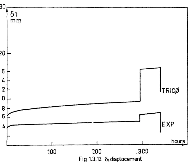
The results are presented on table 1.3.3 and

figures 1.3.12, 1.3.13, 1.3.14, 1.3.15, 1.3.16. The comparison with experimental results shows that these computations over estimate the displacement. This difference is supposed to come for the material data which do not seem to take in account the metallurgical charges of the elbow material which was

rolled , welded and hot bended. Some complementary work was conducted with ASME material data. These results are presented in Part 3 of this report.

Step number 5 10 15 20 25 30 35 39 44 46 49 51 time (hours) 0 5 10 55 100 169.64 293.29 295 295 312,26 339 339

h

(mm) 5.71 6.251 6.507 7.373 7.732 8.157 8.491 8.685 14.956 15.078 15.262 10.324 62 (mm) 3.526 3.857 4.012 4.55 4.775 5.039 5.246 5.365 9.465 9.54 9.652 6.77 63 (mm) 8.7 9.518 9.903 11.225 11.776 12.425 12.933 13.226 23.079 23.264 23.543 16.248 \ (mm) 1.092 1.197 1.248 1.411 1.478 1.559 1.623 1.66 2.745 2.769 2.805 1.777

e

(lO~3rd) 15.15 16.58 17.25 19.56 20.52 21.65 22.53 23.05 40.06 40.38 40.87 28.04

Tableau 1.3.3 - Calculated displacements 1.3.3.2 Strains

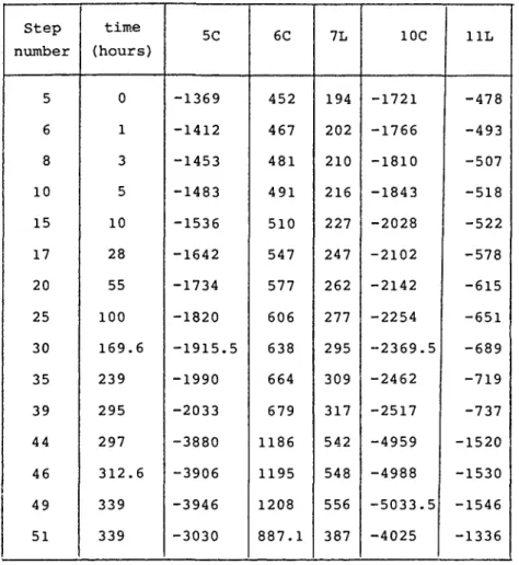
The computed strains are given for the strain gages located on figure 1.3.17. The table 1.3.4 gives this values in micro deformation in function of time. The number of the gage corresponds to the number on figure 1.3.17.

Step number 5 6 8 10 15 17 20 25 30 35 39 44 46 49 51 time (hours) 0 1 3 5 10 28 55 100 169.6 239 295 297 312.6 339 339 5C -1369 -1412 -1453 -1483 -1536 -1642 -1734 -1820 -1915.5 -1990 -2033 -3880 -3906 -3946 -3030 6C 452 467 481 491 510 547 577 606 638 664 679 1186 1195 1208 887.1 7L 194 202 210 216 227 247 262 277 295 309 317 542 548 556 387 IOC -1721 -1766 -1810 -1843 -2028 -2102 -2142 -2254 -2369.5 -2462 -2517 -4959 -4988 -5033.5 -4025 11L -478 -493 -507 -518 -522 -578 -615 -651 -689 -719 -737 -1520 -1530 -1546 -1336

Table 1.3.4 Calculated strains

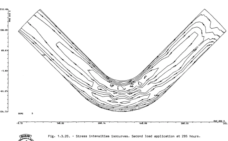
1.3.3.3 Stresses

The stress distribution is represented by the Von Mises stress intensity isocurves. A map of theses isocurves is given at the beginning and at the end of each load. Figure 1.3.18 for the initial load, figure 1.3.19 after 295 h, figure 1.3.20 at 295 h for the second load and figure 1.3.21 after 44 hours of hold time for the second load. The same maps are shown in close

13.4 Conclusions

The results presented for the Elbow-pipe assembly benchmark problem are very different from the measured values as given in reference 6. The deflection curves and strain curves in function of time have the same shape but the end values differ by a factor of 2 on total displacement (or a factor of 3 on creep displacement). Does the material data used in the 'computation correspond to the elbow material which was

subjec-ted to some metallurgical charges during the elbow manufactu-ring ?

3.2 PIPING BENCHMARK PROBLEMS COMPUTER ANALYSIS WITH THE CEASEMT FINITE

ELEMENT SYSTEM by

H. Bung, G. Clement, A. Hoffmann and H. Jakubowicz

This section presents results for the analyses of all three International Piping Benchmark Problems. An inelastic analysis of each problem was performed using a full three-dimensional shell analysis (TRICO code) and a simplified piping analysis based on beam theory

PIPING BENCHMARK PROBLEMS

COMPUTER ANALYSIS WITH THE CEASEMT FINITE ELEMENT SYSTEM

H. BUNG, G. ..CLEMENT, A. HOFFMANN, H. JAKUBOWICZ

Les informations contenues dans ce document sont reservSes aux destinataires nommement designes. Elles ne peuvent

recevoir aucune autre diffusion sans 1'autorisation expresse du Departement des Etudes Mecaniques et Thermiques.

FOREWORD

In accordance with recommandations, at the 1976 IWGFR specialists' Meeting on High-Temperature Structural Design, three experimental benchmark piping problems were selected. The D.E.M.T (Departement des Etudes Mecaniques et Thermiques) of the French Atomic Energy Commission has contributed to this benchmark effort by computing the three proposed problems.

Two different types of analyses were conducted for each problem. Firstly a full three dimensional shell analysis was performed then a simplified piping analysis method is used. The comparison of these twc analyses with the experimental results and between themselves permits not only to assess non linear finite element analysis for piping but also the advan-tages and limitations of simplified methods.

This report is divided in three parts. The first part presents the three dimensional analyses ror the benchmark problems. The second part presents the simplified piping ana-lysis of the same problems. The third part is devoted to the comparaison between the two analysises.

The first and second parts present the respectively used computer codes and a brief summary of the theories used in them. Special mention is made of the global method and of the e Hoffmann method for non linear analysis. The elbow element of the simplified method is described. Input and output of both codes are presented. Then the three benchmark problems are described with all relevant data for the computation. The finite element idealisation is given and the results are shown on

tables and diagrams. The computed results are compared to the measured results.

The third part presents the hypothesis made to explain the observed differences between the three dimensional computa-tion and the measured data. Then are explained the differences

between the two types of analyses. All these explanations are supported by further computations with different shapes, mate-rial data or thicknesses. A cost effectiveness analysis is made for the two types of analysis methods.

CONTENTS

Pages FOREWORD. 0 . 1 PART ONE - P I P I N G BENCHMARK PROBLEMS ANALYSIS WITH THE THREE DIMEN-SIONAL SHELL ANALYSIS COMPUTER CODE T R I C O .

1 . - A three dimensional e l a s t i c - p l a s t i c - c r e e p shell analysis program.

1 . 1 . - Introduction. 1.1 1.2.- Description of the code TRICO. 1.1 1 . 2 . 1 . - General features. 1.1 1.2.2.- The global method. 1.2 1 . 2 . 3 . - The £*-Hoffmann method 1.5 1.2.4.- Material data input. 1.15 1 . 2 . 5 . - Input and output of TRICO. 1.17 1.3.- Elbow-pipe assembly subjected to in-plane moment 1.17 loading a t 593° C. 1 . 3 . 1 . - Problem description. 1.17 1.3.2.- The f i n i t e element i d e a l i s a t i o n . 1.20 1 . 3 . 3 . - Results. 1.22 1.3.4.- Conclusions. 1.25 1.4.- Elevated temperature e l a s t i c - p l a s t i c - c r e e p t e s t of an elbow subjected to in plane moment loading. 1.51

1 . 4 . 1 . - Problem description. 1.51 1.4.2.- The f i n i t e element i d e a l i s a t i o n 1.53 1 . 4 . 3 . - Results. 1.55 1.4.4.- Conclusions. 1.55 1.5.- Room-temperature e l a s t i c - p l a s t i c response of a thin walled elbow subjected t o in plane bending loads. 1.69

1 . 5 . 1 . - Problem description. i.(>9 1. 5. 2. - The finite element idealisation 1.70 1. 5. 3. - Description of the implementation of large

displacements in the £ -Hoffmann method for non linear

structural analysis 1.73 1.5.4. - Results 1.76

PART TWO - PIPING BENCHMARK PROBLEMS ANALYSIS WITH A SIMPLIFIED PIPING ANALYSIS METHOD.

2.- A simplified method for non linear piping analysis.

2.1.- Introduction. 2.1 2.2.- Description of the simplified piping analysis

computer code TEDEL. 2.1 2.2.1.- General features. 2.1 2.2.2.- The global method applied to pipes. 2.2 2.2.3.- The elbow element. 2.5 2.2.4.- Other features. 2.8 2.2.5.- Input and output of the TEDEL computer code. 2.8 2.3.- Elbow-pipe assembly subjected to in-plane moment

loading at 593° C. 2.11 2.3.1.- The finite element idealisation. 2.11 2.3.2.- Results. 2.13 2.3.3.- Conclusions. 2.17 2.4.- Elevated temperature elastic-plastic-creep test of an elbow subjected to in-plane moment loading. 2.43

2.4.1.- The finite element idealisation. 2.43 2.4.2.- Results. 2.45

2.5.- Room-temperature elastic-plastic response of a

thin walled elbow subjected to in plane bending loads. 2.52 2.5.1.- The finite element idealisation. 2.52 2.5.2.- Results. 2.55 2.5.3.- Conclusions. 2.56

PART THREE - ANALYSIS OF BENCHMARK TESTS AND COMPUTER RESULTS. 3.- Evaluation of the benchmark problems. 3.1

3.1.- Introduction. 3.1 3.2.- Influence of material data. 3.2

3.3 - Influence of straight parts on elbows. 3.7

3.4 - Influence of geometrical data. 3.11

3.5 - Cost effectiveness. 3.17

3.6 - Closure. 3.19

PART ONE

PIPING BENCHMARK PROBLEMS ANALYSIS WITH THE THREE DIMENSIONAL SHELL ANALYSIS

COMPUTER CODE TRICO

1 A THREE DIMENSIONAL ELASTIC-PLASTIC-CREEP SHELL ANALYSIS PROGRAM

1.1 Introduction

The TRICO shell analysis computer code is part of the CEASEMT finite element system. It has access to all of this system capabilities. This system is caracterised by a modular architecture especially designed for non linear and dynamic structural problems. A complete library of elements is available as well as a huge capability of pre and post-processors for two and three dimensional problems.

The COCO pre-processor (reference 3) is a mesh generator with its own geometrically oriented language. The TEMPS and ESPACE post-processors (reference 4) are used to display graphically all relevant results respectively in time for a given point and in space for a given time.

1.2 Description of the code TRICO (references 1, 2)

1.2.1 General features

As most of the CEASEMT system programs the TRICO program is based on the finite element method. The TRICO program uses a flat three nodes triangulare constant stress element. Each node has six degrees of freedom. A truss element is also included and can be used in connection with the plate element.

The TRICO program can solve static or dynamic problems. It can search for eigenvalues or give the response to any

excitation or to a varying load by time step integration. It can solve Elastic-plastic-creep analysis with large displace-ments as well as problems in thermoplasticity.

Due to its dynamic storage allocation capability, the TRICO program can solve problems with a large number of unknows. Its limits being those of the out of core storage of •che computer center.

The loading conditions and boundary conditions are numerous and general enough for all engineering needs. It is possible to apply concentrated or distributed forces and

moments as well as pressure, dead weight or thermal loads. The displacements can be imposed in any direction. Relations between displacements or between forces and displacements are easily taken in account as well as the symetry conditions.

1.2.2 The global method (Ref.9)

The basis of this formalism is the notion of genera-lised stresses and strains introduced by Prager (reference 18). These generalised stresses and strains are placed in duality by a bilinear form expressing the virtual work. The equations of plasticity are then expressed directly in terms of these generalised stresses and strains.

For the plate (or shell) element the generalised stresses are the membrane tensions (N. , N~, N,) and the bending moments (M1# M2, M , ) . Corresponding to these stresses are the generalised strains defined by membrane strains (e., e_, e3) and curvature variations (x-., x^i Xo) •

To define a generalised yield surface the second order invariants of the generalised stresses deviator are used in conjonction with the Von Mises criterion. The three invariants are

N2 =

M2 =

MN cose = NjM + - 0.5(M1N2+M2N1) +

and the yield surface is an expression of the form

F(M,N,cos0,ii1,y2,...) = 0

where y , y2, ... are material history parameters.

Hill's principle for plastic flow applied to these relations produces the following relations

/ de, 3F N -0.5N 1 3F M -0.5M i. ^ . X dA de2 dA de3 dA d xi dA dX2 dA dx3 3N 3F 3N 3F 3N 3F 3M 3F 3M 3F N N2-0. N 3 N3 , N M - 0 . M M

2~°"

M 3 M3 , 1 N 5 M2 1 N N 3F 3cosG 1 M .1 M 3F 3cos0 3F 3cos0 3M3 ) M 3F 3cos0 3 cos'P 3N3 M 2 " 1 M N1- 0 . 5 N2 N N -O.5NJ N dA 3M M M 3cosG N

As usually dA is obtained by identifying the relation between equivalent generalised stress and strain intensities to the tensile curve.

In practice in the computer program these generalised stresses and strains are normalised to stress and strain quan-tities by taking in account the thickness of the plate or the shell.

The hardening law can be either one of the following rules : isotropic hardening, kinematic hardening or a multi-layer model.

Then the usual initial stress method, with some

improvements described below, is applied to solve by increments and iterations these non linear equations. For a load increment AF the static equilibrium equation must obviously be satisfied.

This is accom-plished by the so called "extsnal iterations". If the associated stress distribution does violate the yield criteria in some part of the structure, the stress must be brought back on the stress-strain curve by allowing plastic flow in that part. This is accomplished by the so called "internal iterations".

To be more specific let AF be the load increment and AU the displacement increment. Then £ K J {AU} = {AF} whereJ^K^ is the stiffness matrix. If the yield criterion is violated the internal iterations will produce a plastic flow increment

Ae^. To satisfie equilibrium a load increment

is computed where {e^} = C % 3 W '• tofe'} = \psn~\ {em>, m is an element number and Vm, the volume of the element. And then an external iteration is performed that is to say the

[K] {AU}2 = {AR} + {AFp}1

The yield criterion is then verified again and so on. The iterations are stopped when {AFP} = {AFP} or if they differ only by a small amount.

1.2.3 The e*-Hoffmann method

At an equilibrium position the equation

[ B ] T

{a

Q

} =

{FQ}

(1)

is verified. Let {dF} be an infinitesimal increment of load then

[ B ] T {0} = { FQ} + {dF} (2)

if {a} = {a } + ida} then it can be deduced that

[ B ] T {da} = {dF} (3)

But {da} = [XI {cleel= M ({det} - {dep}) (4)

and {det} = O H {du} (5)

where ee, e , ep are the elastic, total and plastic strains an u the displacement. Finally the incremental equilibrium equation can be written as

[ K ]

{du} =

[ B ] T [ D ]

[B]

{du} ={dF} +

[B]

T [D]

{de

P

}

(6)

The Prandtl-Reuss equation for the Von Mises yield criteria can be written as

{de

p

} =

[ M ] i2l

d£

*

(7)

CXJ =

1 2 1 2 0 0 0 1 2 1 1 2 0 0 0 l-l 1 2 1 0 0 0 0 0 0 3 2 0 0 0 0 0 0 3 2 0 0 0 0 0 0 3 2

thus equations (4) and (7) produces

{da} =

-

[D] [M]

(8)

and dividing by de a fondamental equation is obtained

- W

de

(9)

with JX) = [ D ] [ M ] and {dot} = [D] |d£

fc

} .

This differential equation is valid only if de jt 0. To summarise the previous discussion the following two equations must be integrated in order to solve the plasticity problem :

if a*\{o} + {da}) < f(e*) then de* = 0 ana {da} = { d a * } ^ ] {du}

if a*{{a) + {da}) > f (e*) then de* > 0 and {•

de* de

-

[A] ^Ta* where f is the yield surface.

For a finite increment of load {DR} the first external iteration produces the first displacement by

[ K ] { A U }X = {AR} (10)

and the stress increment is known by

{Aat} = [A] { A U }1 (11)

If a* ({aQ} + {Aot}) < f(e*o) then Ae* = 0

and {Aa} = {Aat}.

But if a* ({aQ} + {Aat}) > f(e*Q)then Ae* > 0 and {Aa} is given by the relation

a* ({oo} + {Aa}) = f(e*o + Ae*)

which says only that the stress is on the tensile curve at the end of the load step.

The problem now is how to integrate the differential stress equation between e and e + Ae with

. e equivalent strain at the beginning of the load step

. e + Ae equivalent strain at the end of the load step

. {a } stress at the beginning of the load step

. {a } + {Aa} stress at the end of the load step

1.2.3.1 The fondamental hypothesis dafc

The value of {——} is not known so it will be supposed to be constant on the e £e , e * + Ae ]] interval and equal to { — — } . This consists only to assume that the stress

Ae*

To solve the differential system t da de Aa Ae {a} a (12)

a diagonalisation is performed on the A matrix whose eigenvalues are X = 0 and X_ = X, = X. =

ding eigenvectors are

= X, = -~. The correspon-Vl = 1/V5 1/V3 l/VT 0 0 0 V2 = 1/V2~ -1/V2" 0 0 0 0 V3 " l/VS" i/Ve -2/V6 0 0 0 V4 -0 0 0 1 0 0 V5 = 0 0 0 0 1 0 V6 = 0 0 0 0 0 1

In this base the {a} vector has a. components and

{a} = a. {v } 1 x

thus the differential system can be written da. Aa.t 1 _ J-. * J-. * de A E a. * a (13)

these equations are uncoupled and can be solved separately. The equations are analyticaly integrated and the solutions included in the computer program. Two cases will be developped perfec plastic material and hardening material.

1.2.3.2 Perfect plastic material

The solutions of the differential equations are

X,e Aa*

a (e ) = C exp(- - ± — ) + ^ — i _

the C constant being given by the relation

(14)

o. is the stress value at the beginning oL the load step o

expressed in the base {v±} of eigenvectors of [ V ) - Then

a, (e*) k Ao*fc Xi * 1o Ai Ae* k ° . k ^ i *

e*)) + (15)

at the end of the load step (in fact at e * + A c * ) , where 6

= 1 {v.}.

The only unknow in the last equation is Ae . Its value is determined by writting than the stresses o. are on the stress-strain curve. That is

o* •({oi}) = k ₍₁₆₎

The Newton-Raphson iterative method is used to solve this non linear equation in Ae . Only a few iterations (2 or 3) are necessary. This method is shown schematically on figure

1.2.3. * "~

1.2.3.3 Hardening material (isotropic case)

In this case a is not any nore a constant in equation (13). In the Ceo*r e o* + A e* 3 interval 0* does increase and

this variation is accounted for approximatively.

A limited expansion to the first order, in Ae , of equation (15) and of the tensile curse is made and this leads to

IT

A e } (17) and a* = aQ* + h Ae* where h = ( de* e

the tangent to the tensile curve at e (18)

This set of equations (17 and 18) is solved in Ae and a point (a, , A E , ) is obtained as shown on figure 1.2.4.

Fig 1.2.4 - Solution of equations 17 and 18.

The internal iterations are carried on now on equations (15) and (16) as in the perfect plasticity case but with the mean valve CJ * = k = j ( o * + o *) for the load step. This choice does verify the flow equations only in average on the load step but the error which is introduced is very low.

At the end of the internal iterations the stresses

The new value e + Ae is known as well as the plastic defor-are given by {a } + {Aa} and they defor-are on the stress-strain curve. The new value e

mation variation.

{Aep} = [ D ] "1 ({Aofc} - {Aa})

The plastic load {AFP} necessary to reeguilibrate the structure is then given by

{AFP} = z I C B J 1 ({Aa/} -{Aam}) dVm m vm

This force is added to the second member of the equi-librium equation

D O (AU} = {AR} + {AFP}

which is solved by external iterations.

1.2.3.4 Convergence criteria. An acceleration method

The external iterations are stopped when {AFP} does not change any more. That is done in the computer program by the following criteria. Let a be the value of a (a + Aa -Aa

fl Lj M&M ^^ * ^ XX XX

and a .. the value of a (a + Aa,, - Aa , ) . Then these n—l o n n— l

iterations are stopped when

i •«*-:-! i

Pn = X ^ Pmax

V

for all the elements and where p _= v is the convergence criteria supplied by the user.

The same method applies to the internal iterations but with pm /_ as convergence criteria.

Depending on material caracteristics this convergence can be slow. An acceleration method based on the following extrapolation method was then included in the program.

Let Ae be the variation of equivalent plastic

deformation obtained at the issue of the n external interation the associate

is defined by

and the associated internal iterations. The rate of convergence -rn

= A en " A en-1 n * *

A e

n - r

Ae

n-2

This rate is suppose to stabilise after only a few iterations. At the user's demand every m iterations the limit of the Ae n sequence is then calculated by

T =

Ae*_! - Ae~_2

em-and

Ae* = •—- (Ae - T Ae ,)

•1-T m m-1

which is the limit of the geometric sequence. Then the plastic deformations are modified in the same proportions

7

a eni

(The upper index p is for plastic) and the corresponding plastics loads {AFP} are used for the following external iterations.

For some problems if this extrapolation method fails every few iterations the tangential stiffness matrix can be cal-culated at the users demand.

1.2.3.4 Hardening material (Kinematic hardening)

The yield criteria is written F({a-a}) = 0 and the stress-strain curve supposed to be bilinear. The Prager-Ziegler hypothesis is used to determine the hardening parameter {a,} .

{da} = dp ({a-a})

dp is obtained by differentiating the yield surface equation and using the plastic flow equations. That is

{<*£?} = de*p ({o-a}} 3{a-a}

a* = f ({a-ct})

d f({a-a}) = 0 => df T = 0

and {da} = {(a-a)} dp

Then

But for constant a

and

dy = da h de *

where h is the derivative of the tensile curve at e . This modifies the algorithm previously described in the following manner

t {d0}x = {do*} - [ M ] — — {0 - a} o {da} = -^ de*P {0 - a} 1 0* x t}1 - ( [ M ] + h dE*P

where £ l ] is the unit matrix. It is seen that this equation is the equation (8) by changing {o-a} to { o } . The same integration method can then be applied. This method gives simultanously the

solutions of the equation of plasticity and the displacements of the yield surface defined by { d a } .

1.2.3.5 Application to creep problems

A s usually the first step is to write the equation of equilibrium

[>] {0} = {F} (1)

and the equation for the stresses

{0} = {0Q} + [D] ({Aefc} - {AeF}) (2)

The creep flow is given by the following equation {Aef} = / V ^ t _ | f ^ -*dt ( 3 )

on the time interval C^--,* to + At]»

Equations (1) and (2) are combined and as above it is obtained

M O ]

n

= <AF} + CB] [D] {Ae

P

}

Q

+ M M

(4)

and the same iterative method is applied. The question here is how do one obtain {Ae } from (3). The ir

rically conducted with the simple equation

is how do one obtain {Ae } from (3). The integration is

nume-9f •* , 3f .*>

't=t~ VH o T t=t +At_{o v o}

and {Aep} is then put in equation (4). This last equation replaces the internal iterations previously defined. After equilibrium is obtained at the nt h iterate it is necessary to verify that the stress at the end of the time step is the stress which was used to determine {Ae^}. If it is not the case a

new iteration is performed.

1.2.4 Material data input

For plastic or creep analyses the ability to intro-duce easily material datas in various manners is very important. Generaly these data are given point by point, sometimes an

analytical curve- is assumed and they are also cases where it is necessary to smooth and fit the datas by numerical means. In the TRICO program the stress-strain curves are supplied by either two ways : point by point with the other datar related to the problem or by a user supplied subroutine where any type of constitutive equation can be accounted for. The point by

point data are used by TRICO in conjonction with a quadratic inter-polation. The creep data a r e always given by the user supplied subroutine in the form of the function.

* * *

e = 0 (e , a , t, T, ..., ...)

where z is the strain intensity, a the stress intensity, t the time, T the temperature etc ... Any argument of this function can be omitted and other arguments can be added. If the creep data are given point by point the user supplied subroutine must be provided with an interpolation scheme. This way of dealing with creep leaves the designer free to choose any hardening rule

1.2.5 Input and output of TRICO

The input must always begin with some parameters on the number of nodes and elements and other values, to allocate the computer memory necessary for the problem. All the other data are input in free format fields in any order due to the use of code names to specify the different data categories. The input is generaly composed by

- The mesh : coordinates of the points, numbers defining the elements

- The thicknesses of the elements

- Some material properties :

. Young modulus . Poisson's ratio

. Stress-strain curves (if given point by point)

- The loads

- The load and time increments

- The boundary conditions

- Parameters for non linear analysis : maximal number of itera-tions , convergence criteria

- Parameters for selection of the printed output.

The results are listed or stored on computer files for latter retrieval by post-processor codes. They can be visua-lized on graphic display units, hard copy or plotters.

These post-processor codes can be used either by the batch processing mode or the interactive time sharing mode.

All input data are printed. Then for each time or load steps the following results are printed :

- number of plastic elements,actual convergence error, maximal stress and strain intensities. Actual loads and time incre-ments. Number of iterations.

- At selected elements : the principal strains and curvature variations.

For selected time or load steps the following results are printed

- The displacements and rotations

- The boundary reactions

- The principal stresses and moments

1 3 Elbow-Pipe Assembly Subjected to&In-plane Moment Loading at 593°C

1.3.1 Problem description (ref. 6)

1.3.1.1 Geometry

The Elbow-pipe Assembly tested at Battelle-Columbus Laboratories is a 101.6 mm sched-10 90° elbow with a 152.4 mm bend radius welded to two 324 mm lenghts of sched - 10 pipes.

(Fig. 1.3.1). The elbow wall thicknesses and diameter were measured at selected grid points (table 1.3.1 and Fig. 1.3.2).

a 0° 22.5° 45° 67.5° 90° Wall thicknesses in mm <j>=0° 3.02 2.74 2.76 3.37 2.79 90° 3.2 2.84 2.54 2.81 3.07 180° 3.12 2.94 2.94 2.99 3.12 270° 2.97 3.40 3.50 3.40 3.02 Outside diameter 0° to 180° 114.25 114.50 114.78 115 115.34 90° to 270° 114.88 114.75 114 114.22 113.66

Table 1.3.1 - Dimensions of elbow

The average wall thickness is 3 mm and average outside diameter is 114.53 mm. The pipe legs have a wall thickness

of 3.07 + 0.05 mm, an outside diameter of 114.25 + 0.25 mm and a length of 323.85 mm.

A rigid frame shown on fig. 3.1 is used to apply the loads.

1.3.1.2 Loads and boundary conditions

As system of dead weights was used to load the assembly. These loads produce a constant moment in the assem-bly. On figure 1.3.3 the loads are noted as Fj and F_. The load histogram is shown on figure 1.3.4. A first load of 1382 N is applied on each loading point producing a bending moment of 843 Nm. The specimen is held at this load for 295 hours. The load is then increased to 1827 N producing a bending moment of 1114 Nm. This load is held for another 44 hours. At this time the test is ended. The temperature during all the test is maintained at 593°C + 5.6°C.

The Elbow pipe asseitibly is rigidly fastened at the other end.

1.3.1.3 Material

The elbow and pipe legs are made of type 304 stainless steel. The material properties are given in reference 5.

9 Young modulus 149 652 N/mm Poisson's ratio 0.3

The stress-strain curve at 593°C is given by the following formula

ep = 4.59 x lO"4 1 a9'3 3 7 7

where a is in psi and Ep the plastic strain is in/in. The tensile curve values are given below in table 1.3.2 and the correspon-ding graphe is shown on fig. 1.3.5.

a ksi 6.5 8.5 9 10 10.5 11 11.5 12 15 17 a (N/mm2) 44.8 58.7 62.1 69 72.4 75.8 79.4 82.8 89.7 117.2 e (mm/mm) 0.0002996 0.0006 0.0008 0.0015 0.0021 0.0030 0.0043 0.0062 0.0125 0.1468

The creep data are given by the reference 5 table 2.

1.3.2 The finite element idealisation

1.3.2.1 Geometry

Half of the elbow pipe assembly due to symmetry

conditions) is meshed with 770 triangular elements and 432 nodes. The mesh, the element numbering and nodal numbering are

presented on figures 1.3.6, 1.3.7 and 1.3.8.

Each element is given its appropriate thickness. The eguithickness lines are represented on figure 1.3.9.

The frame at the free end was not meshed but repre-sented by a rigid flange. This flange is reprerepre-sented in the mesh by the last row of elements (74 9 to 770) which were given a 45 mm thickness.

1.3.2.2 Loads and boundary conditions

The forces are introduced directly on the mesh on points number 421 and 432. They are given a value taking in account the effect of the beams length. That is

F

F * x R = — x 304.8 mm 1 2

where R is the mean radius of the pipe, and, due to the symmetry condition, only half of the load is applied.

* 1382 x 304.8 _ „, Fl = 2 x 55.63 - 3 7 8 6-0 3 N The same value is given to F_ .

By the same formula the second load is obtained as 5005.12N.

The boundary conditions as mentionned previously are symmetry conditions for the XOY plane and of the clamped type conditions for the fixed pipe end. This was imposed by setting to zero value all the degrees of freedcmn of nodes 1 to 12 and

symmetry condition an nodes 13, 25, ..., 421 and 24, 36, ..., 432.

1.3.2.3 Material

The stress-strain curve was entered point by point with the values of table 1.3.2.

The creep data were replaced by a similar matrix but with strain rates. These rates were calculated from

table 1.3.3 by taking the ratio between strain differences and time differences for a given stress level. (For exemple at a stress of 14 Ksi between the 50 t h an(j ioO t h hour the rate is 89x10 in/in/hour). These rates were included in a user

supplied subroutine where linear interpolation between stress levels was programmed.

1.3.2.4 Miseellanious data

The maximum number of iterations is set to 23 and the convergence criteria T to 10"^. The total number of

max

time and loadincrements is 51 (Fig. 1.3.10). The first five steps are used to impose the initial load at constant time

(no hold time). Then the following time table is used : between 0 and 10 hours 10 steps

between 10 and 100 hours 10 steps between 100 and 295 hours 14 steps

Then the load is incremented in five steps at cons-tant time and between the 295t h and 339t h five time steps are used. The unloading is made in two load steps at 339 hours.

1.3.3 Results

1.3.3.1 Displacements

Due to the idealisation some additional computation are necessary to provide typical displacements that are compa-rable to the set presented in the Benchmark problem. The

quantities $ , 62/ 6_, 6 and 9 as defined in reference 6 and on figure 1.3.11 are obtained by taking the mean values of u and vB,the displacements in the x and y directions respec-tively, ,of the points 425 and 426 of the mesh. The following formulas are applied

6._ = vA - 304.8 0A

62 = " VA ~ 3 0 4-8 QA 63 = - 165.1 0A + uA

e =

-The results are presented on table 1.3.3 and

figures 1.3.12, 1.3.13, 1.3.14, 1.3.15, 1.3.16. The comparison with experimental results shows that these computations over estimate the displacement. This difference is supposed to come for the material data which do not seem to take in account the metallurgical charges of the elbow material which was

rolled , welded and hot bended. Some complementary work was conducted with ASME material data. These results are presented in Part 3 of this report.

Step number 5 10 15 20 25 30 35 39 44 46 49 51 time (hours) 0 5 10 55 100 169.64 293.29 295 295 312,26 339 339 (mm) 5.71 6.251 6.507 7.373 7.732 8.157 8.491 8.685 14.956 15.078 15.262 10.324 62 (mm) 3.526 3.857 4.012 4.55 4.775 5.039 5.246 5.365 9.465 9.54 9.652 6.77 (mm) 8.7 9.518 9.903 11.225 11.776 12.425 12.933 13.226 23.079 23.264 23.543 16.248 (mm) 1.092 1.197 1.248 1.411 1.478 1.559 1.623 1.66 2.745 2.769 2.805 1.777

e

(10"3rd) 15.15 16.58 17.25 19.56 20.52 21.65 22.53 23.05 40.06 40.38 40.87 28.04

Tableau 1.3.3 - Calculated displacements

1.3.3.2 Strains

The computed strains are given for the strain gages located on figure 1.3.17. The table 1.3.4 gives this values in micro deformation in function of time. The number of the gage

Step number 5 6 8 10 15 17 20 25 30 35 39 44 46 49 51 time (hours) 0 1 3 5 10 28 55 100 169.6 239 295 297 312.6 339 339 5C -1369 -1412 -1453 -1483 -1536 -1642 -1734 -1820 -1915.5 -1990 -2033 -3880 -3906 -3946 -3030 6C 452 467 481 491 510 547 577 606 638 664 679 1186 1195 1208 887.1 7L 194 202 210 216 227 247 262 277 295 309 317 542 548 556 387 IOC -1721 -1766 -1810 -1843 -2028 -2102 -?142 -2254 -2369.5 -2462 -2517 -4959 -4988 -5033.5 -4025 11L -478 -493 -507 -518 -522 -578 -615 -651 -689 -719 -737 -1520 -1530 -1546 -1336

Table 1.3.4 Calculated strains

1.3.3.3 Stresses

The stress distribution is represented by the Von Mises stress intensity isocurves. A map of theses isocurves is given at the beginning and at the end of each load. Figure 1.3.18 for the initial load, figure 1.3.19 after 295 h, figure 1.3.20 at 295 h for the second load and figure 1.3.21 after 44 hours of hold time for the second load. The same maps are shown in close

13.4 Conclusions

The results presented for the Elbow-pipe assembly benchmark problem are very different from the measured values as given in reference 6. The deflection curves and strain curves in function of time have the same shape but the end values differ by a factor of 2 on total displacement (or a factor of 3 on creep displacement). Does the material data used in the 'computation correspond to the elbow material which was

subjec-ted to some metallurgical charges during the elbow manufactu-ring ?

304.8mm

304.8 mm

324 mm

Rigid frame

Section A A

3QA.8mm

165.1 mm

-rigid structure

pipe

Nm

11U

843

0) o

E

c 0) a

Time (hours)

295

339

Fig. 1.3.4 Load histogram

(isd) o o o o o o o o o in o »-t •H +J fH 3 M C •H •o a o t/l O rt o t-l o +J CJ tn o a to c 01 CJ •H ^^ o <u

CD CO DO

10 steps 10 steps Usteps

[5]

steps numbers are in brackets

j L

10 100

295

[50]

(hours)

339

u

vJ65.1mm

dements 425 and 426)

'/////////////A

_{simulated rigid flange}

VD

-pipe

100

200 .3C0

.10

5

-1 -1

r "

i

TRICO

Experiment

i 00

100

200 300

Fig. 1.3.13 5

7

displacement

400

c

0)

o

"a.

.in CO «o

^t

*-.

CO

1

-200 300

Fig. 1.3.15 6

y

displacement

nr\/

U.UA

0.03

0.02

Q01

e

-1 -1

Trico

-experiment

100

0 rotation

Fig 1.3.16

300 time (hours)

Strain Gage Length - 0.375" C *= Circumferential.

L «= Longitudinal

Gages are on outside surface

I

154.11-' O .p-BUNC 1 4 4 * . 0 S Q t . 0 3 fIXE OES R 745.91 zgi.

BUNG 5

59S703 m i . 91

BUNG 5

> , ' \ \ {

z S3o 3/a A -• r • - . - ~ r -

-f-O)

to

o

rH

CJ

to

o

1.4 Elevated-Temperature Elastic-Plastic-Creep Test of an Elbow Subjected to In-Plane Moment Loading (Ref.7)

1.4.1 Problem description

1.4.1.1 Geometry

This assembly was a 304.8 mm, sched-20, 90° elbow and pipe fabricated from type 304 stainless steel. The geometry is presented on figure 1.4.1. The elbow and pipes wall thicknesses were measured and supplied in addenda 1 to reference 7. These values are reprodu-ced in table 1.4.1. The positions of the grid points for the thickness measurement are given on fig. 1.4.2. The pipe numbers are defined on

figure 1.4.1. : Pipe number : 1 : 2 : 3 Outside "diameter (mm) . 318.5 318.5 318.5 wall : thickness (mm) 6.5 : : 6.5 : : 10. : Table 1.4.1 (a)

The length of pipe 1 is 742.8 mm the length of pipe 2 and 3 are supposed to be respectively 678.4 mm and 864 mm.

1.4.1.2 Loads and boundary conditions.

A transverse concentrated force is applied at one end of the assembly producing an in-plane bending moment in the elbow.

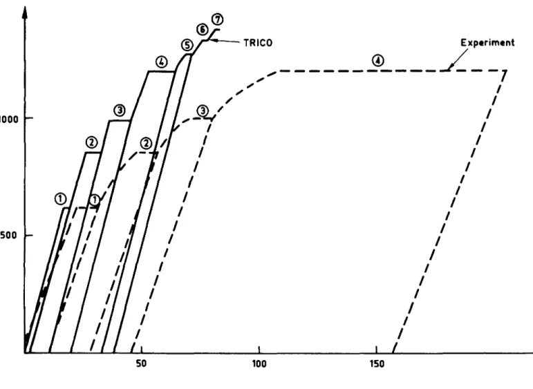
The load history is shown on figure 1.4.3. Seven loads were applied, each load being followed by a period of hold time. For steps 1 to 5 the load was removed at the end of the creep period. For steps 6, the load was increased directly into step 7.