Adaptive Load Balancing Dashboard in Dynamic Distributed
Systems
Seyedeh Leili Mirtaheri1, Seyed Arman Fatemi2, Lucio Grandinetti3
c
The Authors 2017. This paper is published with open access at SuperFri.org
Considering the dynamic nature of new generation scientific problems, load balancing is a ne-cessity to manage the load in an efficient manner. Load balancing systems are used to optimize the resource consumption, maximize the throughput, minimize response time, and to prevent overload in resources. In current research, we consider operational distributed systems with dynamic vari-ables caused by different nature of the applications and heterogeneity of the various levels in the system. The conducted studies indicate that many different factors should be considered to select the load balancing algorithm, including the processing power, load transfer and communication delay of nodes. In this work, We aim to design a dashboard that is capable of merging the load balancing algorithms in different environments. We design an adaptive system infrastructure with the ability to adjust various factors in the run time of a load balancing algorithm. We propose a task and a resource allocation mechanism and further introduce a mathematical model of load balancing process in the system. We calculate a normalized hardware score that determines the maturity of the system according to the environmental conditions of the load balancing process. The evaluation results confirm that the proposed method performs well and reduces the probability of system failure.
Keywords: Load Balancing, Resource Management, Dynamic Variables, Communication De-lay, Distributed System.
Introduction
In the next-generation high performance computing (HPC) systems, the scientific programs are going to get more complex with unpredictable requests what requires large scale and more powerful computing systems [3]. Distributed computing system (DCS) is a promising solution to such demands. DCS consists of a group of computers, each of which has an independent operating system and all are connected through a network [12]. This definition of distributed computing systems is very general and covers all types of purposes for user resource connectivity. Users get connected to resources to receive different facilities and services like computing, file sharing, I/O sharing, and storage. In distributed computing systems with mission of high performance computing, the main concern of managing resources is reaching to minimum execution time and maximum throughput in running scientific/industrial programs [10].
In resource management framework, the load balancer is the key unit in efficient utilization of resources and improving response time [16]. Load balancing is the distribution of load among several computing resources such as computers, clusters, network communication lines, central processing units, or disk drives. The advantages of the load balancing could be categorized as: optimizing resource consumption, maximizing network throughput, reducing response time, and preventing overload in each resource. It is known that using multiple components in load balancing increases reliability and availability [5].
In load balancing mechanism, some parameters have direct impact in efficiency of load balancing operation. A group of these parameters are determined by specifying the status of nodes [1]. Practically, the nodes speed up in executing the commands and their current load are
1Department of Electrical & Computer Engineering, Faculty of Engineering, Kharazmi University, Tehran, Iran 2Kharazmi University, Tehran, Iran
two important factors in specifying the status of the nodes and making decision to distribute the load based on them. It is clear that, the load balancer should migrate and transfer the extra load from over loaded nodes to the ones that are under loaded. Another group of parameters are related to execution of load balancing mechanism that among them specifying the start time of load balancing mechanism is an important issue. In one-shot strategy, when extra load is imposed in the node, the load balancing operation starts to work [11]. The third group of parameters are related to interconnection platform status. The important effective parameter in load balancing mechanism from these parameters is the communication delay between the nodes.
Load balancing should not only be considered in terms of a mechanism that can improve the computing efficiency. Load balancing is a necessity for large scale computing systems. In such systems, the whole computation goal may fail if the load balancing is not applied in the system. on the other-hand, predetermined variables are commonly used in decision-making algorithms by introducing unchangeable formulas and computing algorithms. Therefore, beside efficient and optimized algorithms for load balancing, it is important to introduce a framework dashboard that can also adapt to variation of parameters by choosing different algorithms, dynamically. Therefore, the two usage of load balancing systems are as follows:
1. Reducing critical points in system: In fact, using load balancing improves the system avail-ability. If an adaptive load balancing system is used in the network and a node (hardware or software) corrupts, no failure time is felt from the user’s side.
2. Efficient load distribution by load balancing exploits the full computational power (maxi-mum available) of system elements.
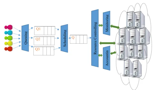
Standard load balancing manager includes five activities: queuing, scheduling, monitoring, resource control and accountants. As shown in Fig. 1, queuing is the first phase of load balancing operation and in this unit the tasks are assigned by user, and the process ends by giving the result of executed tasks to the user. The aim of these five activities is efficient matching of user-specified workload to existing resources by keeping balance the load of the system. The standard process of load balancing manager starts by receiving the jobs from users in queuing unit. After placement of jobs in queues, scheduling unit is activated. Scheduling is a fundamental technique for improving performance in computer systems. The scheduler has to balance the priorities of each job, with the demands of other jobs, the existing system compute and storage resources, and the governing policies dictated for their use by system administrators. Scheduler should be able to deal with different types of jobs such as huge jobs, small jobs, real-time jobs, high-priority jobs, dynamic jobs, static jobs and etc. The scheduler governs the order of execution based on these independent priority assessments.
Figure 1. Standard load balancing manager scheme
and the investigation of Azure Load Balancing system. The effect of communication delay on load balancing is presented in Section 2 and Section 3 includes our proposed task and resource allocation mechanism. The mathematical model and scoring model are presented in Section 4, and evaluation results of the proposed method are presented in Section 5. Finally, Section 6 concludes the paper.
1. Related Works
1.1. Related Researches
Research studies conducted in this area pursued specific goals. The summarized significant goals in the literature are as follows:
1. In some of the studies, the goal is to propose new methods to improve the performance of current algorithms for different environments. These studies investigate the performance of the existing algorithms and proposed combined algorithms derived from the existing ones [15]. Usually, the authors compare the response time of the proposed algorithms with the existing ones by simulating the environment through simulation tools.
2. Some studies focus on load balancing algorithms in particular environments (such as public clouds) [19]. Generally, this approach aims to adapt and optimize load balancing algorithms based on the implementation variables.
3. Some researchers focus on mathematical approaches to improve the performance of load balancing algorithms. For example, heuristic optimization and artificial intelligence tech-niques [8].
One of the main challenges of performing a load balancing process, is the right choice of algorithm. This choice, as mentioned earlier, is influenced by many factors. A lot of studies were conducted to find a proper algorithm. In [9] authors propose a dynamic parallel scheduling al-gorithm for load balancing. Several strategies are proposed to distribute the load using dynamic and distributed load balancing mechanisms, called sender-initiated and receiver-initiated strate-gies. In the sender-initiated strategy, a portion of the load of over-loaded processor is sent to another computing node [2]. In receiver-initiated strategy, the under-loaded processor initiates the transaction by sending a message to other nodes [6]. In [7], authors propose a load balanc-ing mechanism for massive parallel computations based on sparse grid combination techniques. In [18], authors present an optimized load balancing algorithm by organizing the tasks in queues based on task data size and location. The implemented technique is a MATRIX. However, the portion of the load that should be transferred by forming unpredictable events in runtime is not specified. The proposed method in [17], named Slum++, employs multiple controllers so that each one manages a partition of computing nodes and participates in resource allocation through resource balancing techniques. The authors propose a monitoring-based weakly consis-tent resource stealing technique to achieve resource balancing in distributed high performance computing. In [14], authors investigate migration of applications for high performance com-puting by deriving respective requirements for specific field of applications. In [10], authors consider practical parameters such as communication delay and propose an optimized dynamic load balancing algorithm for exasclae distributed computing systems.
1.2. Related Measures
1.2.1. Azure Load Balancing
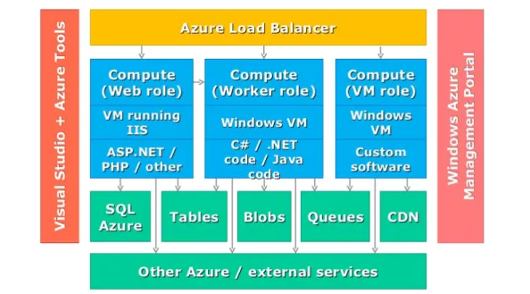
In this section we review the Azure Load Balancing (ALB) system as a successful and practical business case as illustrated in Fig. 2. The ALB system is a load balancing service based on the process as a Service, which provides the highest level of network performance as well as the highest level of availability under UDP and TCP protocols. This system splits the traffic among healthy devices in a cloud structure or among distributed virtual machines. ALB is commonly used in the following cases:
• Splitting traffic of Internet access among virtual machines;
• Splitting traffic among virtual machines in a virtual network, among virtual machines in a cloud service, or among virtual machines and local computers in a local interconnect network; and
• Conducting external traffic on a specific virtual machine.
1.2.2. Required Attributes of ALB
Figure 2. General architecture of Azure Load Balancing
1. Wall Back Time: It represents the maximum allowed runtime for Job. This attribute is accepted in two formats: second and HH: MM: SS. This is an estimated time, and if our work exceeds it, it will be eliminated by the system.
2. Nodes: Through this attribute, the number of nodes and node characteristics are specified. It is also used to specify the number of processors per node or PPN, the number of GPUs per node or GPUN, and the type of node.
3. Memory: This attribute determines the total amount of memory in all nodes. This feature is used in special cases when requiring a high-memory node, or when there is no matching between the number of processors in the node and requested memory.
2. Effect of Communication Delay on Load Balancing
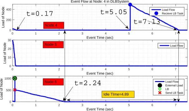
To illustrate the effect of load transfer delay, we consider a scenario and assume that all nodes have 300 initial tasks. The load execution speed is considered to be 200 tasks per second for each node and 100 tasks per second are transferred from one node to another. In this scenario, we assume that the external load is inserted to node 6 having node 4 as its sole neighbor depicted in Fig. 3.
Figure 3. Graph of a sample distributed system model
As depicted in Fig. 4, the node 4 performs all assigned tasks at t=0.17 and is in standby state till t=5.05 when the load from load balancing is reached to node 4. The load balancing is performed in a way that all nodes finish their tasks together. The standby time of node 4 causes extra delay in the system and node 4 finish its assigned tasks at t=7.13 while node 6 ends the tasks at t=2.24. According to the definition of total exertion time, the network execution time for assigned tasks is equal to t=7.13. So, it is obvious to compensate for this load transfer delay and to prevent the standby time in the system [10].
0 1 2 3 4 5 6 7
Event Time (sec)
0 200 400
Load of Node
Event Flow at Node: 4 in DLBSystem
Load Flow Recieve LB Task
0 1 2 3 4 5 6 7
Event Time (sec)
0 10 20 30
Load of Node
Load Flow
0 1 2 3 4 5 6 7
Event Time (sec)
0 500 1000
Load of Node
Load Flow External Load LB Send LB Task
t=0.17
t=2.24
t=5.05
t=7.13
Idle TIme=4.89 Node 5
Node 6 Node 4
3. Proposed Mechanism
In this section, we outline the proposed system. The innovation of proposed mechanism is described in the following two subsections:
• Task allocation process; and
• Resource allocation process
The main procedure is depicted in Fig. 5. First the user needs to specify the resource allocation process to prioritize tasks for execution after determining the intended user algorithm (without the need for coding unlike the existing simulators). In the final step, the user executes the load balancing procedure and views the results.
Figure 5. The general procedures of load balancing in the proposed system
3.1. Entities Participating in the Load Balancing Process
3.1.1. Virtual Servers
The structure of the entity in the database is depicted in Fig. 6. In simple words, each virtual server can have one or more Hardware in this system. Each Hardware has exactly one Hardware Type, and each Hardware Type has one Unit. This structure is used to explain how the load balancing algorithm is implemented.
Figure 6. Conceptual model of virtual servers
3.1.2. Job/Task
completely dynamic manner). We also use this structure to explain how to implement the load balancing algorithm in the following section.
Figure 7. Conceptual model of job/task
3.2. Resource Allocation Process
The proposed system can facilitate implementing the required algorithms and allocating resources in the environment. The general approach is to enable the user to implement algo-rithms and allocate resources without dealing with complex issues (compared to other existing simulators, such as SimGrid [4]), by using the structures described in the following section.
3.2.1. Load Balancing and Resource Allocation Process
The load balancing and resource allocation processes are implemented in two ways that are described separately.
Load balancing process using predetermined algorithms: In this model, the load bal-ancing and resource allocation processes are performed using the following steps:
1. Selecting tasks (jobs) from the task list defined in the system. 2. Selecting servers from the server list defined in the system.
3. Selecting an algorithm from the following algorithms for selecting tasks. 4. Applying the settings for the resource allocation process.
5. Executing the load balancing process using predefined formulas.
In this procedure, the load balancing process is executed according to the selected settings for all available queues of job. However, first, the tasks need to be sorted according to the selected algorithm to form queues. Simply put, the load balancing process is fully executed for all the job queues. After a complete execution, the load balancing process is executed for the next task in the queue for all servers (available in the server queue) according to the server settings. This procedure is summarized in Fig. 8.
Load balancing process using dynamic algorithms: The objective is to create a dy-namic environment for executing load balancing algorithms according to the user requirements. The proposed system provides the ability to implement different load balancing algorithms in runtime through different settings applied by user. This model is depicted in Fig. 9.
4. Mathematical Model of the Proposed System
The load balancing process in proposed system, includes the following steps:
Figure 8.Load balancing process using predetermined algorithms
Figure 9.Load balancing process using dynamic algorithms
requirements. For example, if a job requires four different types of hardware, only the servers that meet these requirements remain in the list.
virtual Server⇒
Distinct(HardwareType in Jobs)∈Distinct(HardwareType in VirtualServere) (1)
Filter 2 on servers: Each hardware type in each server has a total capacity called briefly the Capacity. There is also an in-use value called In Use. For the current job, we filter all servers with the Capacity-In-use value higher than the required value for the job.
ΛHardwareTypeVirtualServer⇒
(Capacity-Inuse) in VirtualServer>0 Λ
(Capacity-Inuse) in VirtualServer>(Consumption) in Job (2)
accordingly, rate each server. That is, the specific score of a hardware type for each hardware type available on servers is calculated as follows:
Hardware Type Score in VirtualServer=
(Capacity-Inuse) of Current Hardware Type in Current VirtualServer max
Current Hardware Type in All VirtualServers(Capacity-Inuse)
(3)
Given the fact that the previous approach leads to the elimination of the unit in computing, we can calculate a server score according to the scores of different hardware types on a server as follows:
Score of VirtualServer=
Hardware Type in VirtualServer index=P i
n
(Capacity-Inuse) of Current Hardware Type in Current VirtualServer max
Current Hardware Type in All VirtualServers(Capacity-Inuse)
(4)
With regard to the score obtained for each server, we can determine the optimal server for the job. Moreover, if the user selects dynamic variable values for participating in the load balancing process (for each server), the values participated in the computing process according to their data entry style in the software as follows:
Final Score of VirtualServer=
Hardware Type in VirtualServer index=P i
n
Hardware Type Score[i]
+
Dynamic Variable in VirtualServer index=P i
n
Dynamic Variable[i]
(5)
5. Evaluation Results
5.1. Practical Example
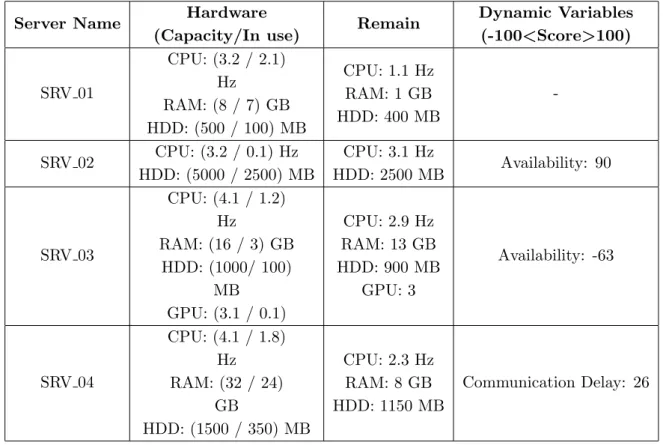
In this part a practical example of the execution of the load balancing process is presented. It is assumed that, according to the settings outlined, the load balancing process is started in the system, using both dynamic and predetermined formulas. The current job specifications (Top job in closed queue) and the available server specifications in server queue are presented in Tab. 1 and Tab. 2, respectively.
Table 1.Job 01 Specifications
Job Name Hardware Requirements
Job 01
CPU:0.5 Hz RAM: 3 GB HDD: 200 MB
Table 2.Specification of Virtual Servers
Server Name Hardware
(Capacity/In use) Remain
Dynamic Variables (-100<Score>100)
SRV 01
CPU: (3.2 / 2.1) Hz
RAM: (8 / 7) GB HDD: (500 / 100) MB
CPU: 1.1 Hz RAM: 1 GB HDD: 400 MB
-SRV 02 CPU: (3.2 / 0.1) Hz HDD: (5000 / 2500) MB
CPU: 3.1 Hz
HDD: 2500 MB Availability: 90
SRV 03
CPU: (4.1 / 1.2) Hz
RAM: (16 / 3) GB HDD: (1000/ 100)
MB GPU: (3.1 / 0.1)
CPU: 2.9 Hz RAM: 13 GB HDD: 900 MB
GPU: 3
Availability: -63
SRV 04
CPU: (4.1 / 1.8) Hz RAM: (32 / 24)
GB
HDD: (1500 / 350) MB
CPU: 2.3 Hz RAM: 8 GB HDD: 1150 MB
Communication Delay: 26
is not given any score, because here this hardware type is not needed. The score is calculated between the servers remaining in the queue according to each hardware type based on that hardware type maximum. The score for SRV 03 and SRV 04 is illustrated in Tab. 3.
Table 3.Comparing Score for SRV 03 and SRV 04
Hardware Types In Current Job Maximum Remain Between All Hardware Type in Servers
Score of SRV 03
Score of SRV 04
CPU 2.9 Hz (SRV 03) 2.9 Hz/2.9 Hz =1 2.3 Hz/2.9 Hz= 0.79 RAM 13 GB (SRV 03) 13 GB/13 GB= 1 8 GB/13 GB= 0.61 HDD 1150 MB (SRV 04) 900 MB/1150 MB =0.78 1150 MB/1150 MB= 1
SUM 2.78 2.39
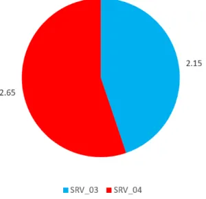
So far, the score of each server is calculated based on the proposed algorithm. Now it is time to apply dynamic variable scores to the system. The result is presented in Tab. 4.
As depicted in Fig. 10 it is clear that the winner server is SRV 04.
5.2. Simulation Procedure
Table 4.Calculating SRV 03 and SRV 04 Score in Dynamic Variable Case
Server Name Dynamic Variable Score
Current Score
Total Score (Dynamic Variable)
Current
SRV 03 -63 /100 = -0.63 2.78 2.15
SRV 04 26 /100 = 0.26 2.39 2.65
Figure 10.General comparison between SRV 03 and SRV 04
and the decision is applied by the same node in this category of algorithms. The central part is a subset of this algorithm. Then according to the described example, the dashboard can play the role of the center in this system. The developed algorithm is based on load balancing process using dynamic algorithms. At first, we consider some basic rules for the existing environment as follows:
Rule 1: Some services have uncertain latency in the system. However, the latency can be generally divided into three categories based on to the range of changes.
• Communication latency of less than 20 milliseconds;
• Communication latency of 21-80 milliseconds; and
• Communication latency of 81-150 milliseconds.
According to the job type in this environment and the execution time, servers with a latency of more than 151 milliseconds are considered to be rejected, and nothing refers to them.
Rule 2: The custodian of the environment in which the load balancing process is implemented is a subset of a major organ. According to this fact, the organization will always keep its most powerful server in reserve, according by order of the same organ, and this fact must be taken into account for the load balancing process.
Rule 4: Because of the geographical conditions of the area in which the servers are located, they are subject to high humidity. Therefore, humidity control devices are used to control the humidity level for the servers in different racks. Currently, it is preferable not to refer the job to some servers (located on the second floor of the building) which should also be considered in the implementation of the load balancing process. Given the limitations and conditions above, we need to implement this algorithm in the environment in such a way that we cover all the aforementioned aspects.
The Solution for Rule 1: The use of dynamic variables. Given the above and the sensitivity and importance of time, we define a dynamic variable called Communication Delay to apply the corresponding servers by using the following rules:
• Communication Delay is zero for servers with a latency of less than 20 milliseconds. So, we are allowed not to apply this variable to this category of servers because it will not affect the computing results;
• Communication Delay is -20 for servers with a latency of 21-80 milliseconds; and
• Communication Delay is -60 for servers with a latency of 81-150 milliseconds.
The Solution for Rule 2: The use of system settings when developing the resources allocation algorithm. This is anticipated when implementing the resource allocation process in the system. The user determines which server is the winner after the execution of load balancing process in the system. After determining the second server as the winner, the company’s most powerful server will be used as reserve.
The Solution for Rule 3: The use of dynamic variables. We can fully cover Rule 3 by defining a dynamic variable called Quality and set it as follows:
• For servers subject to degradation problems, we consider the value of Quality to be -40; and
• For the rest of the servers, we consider the value of this variable to be +40.
The Solution for Rule 4: The use of dynamic variables. We define a dynamic variable called Humidity with a value of -50 for the servers located on the second floor. Now with regard to the above, we can conclude that all the necessary infrastructures required for the implementation of the load balancing process are provided through the proposed solutions.
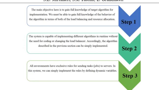
As depicted in Fig.11, the steps to implement a load balancing algorithm using the proposed system are as follows:
1. Full knowledge of the behavior of the algorithm in terms of both of the load balancing and resource allocation.
2. Implementation of load balancing approach and resource allocation approach using the dash-board facilities.
3. Applying the existing limitations and rules to the system by defining related dynamic vari-ables.
Conclusion
Figure 11. General method for implementing load balancing algorithms in the proposed dash-board
designed a rule-based dashboard to manage the load balancing process in real-time runtime. We proposed a scoring system to find the best computing node based on the task specification in an adaptive manner. We showed that our proposed system is capable if change the boundaries and limitations of the system, changing the load balancing process, introducing new variables and removing the existing ones and measuring the running algorithm in the system. We evaluated our proposed system based at a practical implementation. We also presented a simulation based on different rules in a limited environment. Evaluation results proved that the proposed system reduced the probability of the system failure and also determined the maturity of the system according to the environmental conditions of the load balancing process.
This paper is distributed under the terms of the Creative Commons Attribution-Non Com-mercial 3.0 License which permits non-comCom-mercial use, reproduction and distribution of the work without further permission provided the original work is properly cited.
References
1. Arab, M., Mirtaheri, S., Khaneghah, E., Sharifi, M., Mohammadkhani, M.: Improving learning-based request forwarding in resource discovery through load-awareness. Data Man-agement in Grid and Peer-to-Peer Systems pp. 73–82 (2011), DOI: 10.1007/978-3-642-22947-3 7
2. Balasangameshwara, J., Raju, N.: Performance-driven load balancing with a primary-backup approach for computational grids with low communication cost and replication cost. IEEE Transactions on Computers 62(5), 990–1003 (2013), DOI: 10.1109/TC.2012.44
4. Casanova, H.: Simgrid: A toolkit for the simulation of application scheduling. In: Cluster computing and the grid, 2001. Proceedings. First IEEE/ACM international symposium on. IEEE (2001), DOI: 10.1109/CCGRID.2001.923223
5. Dinitz, M., Fineman, J., Gilbert, S., Newport, C.: Load balancing with bounded conver-gence in dynamic networks. In: IEEE INFOCOM 2017 - IEEE Conference on Computer Communications. pp. 1–9 (2017), DOI: 10.1109/INFOCOM.2017.8057000
6. Domanal, S.G., Reddy, G.R.M.: Load balancing in cloud environment using a novel hybrid scheduling algorithm. In: Cloud Computing in Emerging Markets (CCEM), 2015 IEEE International Conference on. pp. 37–42. IEEE (2015), DOI: 10.1109/CCEM.2015.31
7. Heene, M., Kowitz, C., Pfl¨uger, D.: Load balancing for massively parallel computations with the sparse grid combination technique. In: PARCO. pp. 574–583 (2013), DOI: 10.3233/978-1-61499-381-0-574
8. LD, D.B., Krishna, P.V.: Honey bee behavior inspired load balancing of tasks in cloud computing environments. Applied Soft Computing 13(5), 2292–2303 (2013), DOI: 10.1016/j.asoc.2013.01.025
9. Mahafzah, B.A., Jaradat, B.A.: The hybrid dynamic parallel scheduling algorithm for load balancing on chained-cubic tree interconnection networks. The Journal of Supercomputing 52(3), 224–252 (2010), DOI: 10.1007/s11227-009-0288-3
10. Mirtaheri, S.L., Grandinetti, L.: Dynamic load balancing in distributed exascale computing systems. Cluster Computing (May 2017), DOI: 10.1007/s10586-017-0902-8
11. Mohamed, N., Al-Jaroodi, J.: Delay-tolerant dynamic load balancing. In: 2011 IEEE In-ternational Conference on High Performance Computing and Communications. pp. 237–245 (2011), DOI: 10.1109/HPCC.2011.39
12. Mousavi Khaneghah, E., Mirtaheri, S.L., Sharifi, M., Minaei Bidgoli, B.: Modeling and analysis of access transparency and scalability in p2p distributed systems. International Journal of Communication Systems 27(10), 2190–2214 (2014), DOI: 10.1002/dac.2467
13. Patel, P., Bansal, D., Yuan, L., Murthy, A., Greenberg, A., Maltz, D.A., Kern, R., Kumar, H., Zikos, M., Wu, H., et al.: Ananta: Cloud scale load balancing. In: ACM SIGCOMM Computer Communication Review. vol. 43, pp. 207–218. ACM (2013), DOI: 10.1145/2486001.2486026
14. Pickartz, S., Lankes, S., Monti, A., Clauss, C., Breitbart, J.: Application migration in HPC driver of the exascale era? In: High Performance Computing & Simulation (HPCS), 2016 In-ternational Conference on. pp. 318–325. IEEE (2016), DOI: 10.1109/HPCSim.2016.7568352
15. Sharma, M., Yadav, A., Sharma, P.: An optimistic approach for load balancing in cloud computing pp. 27–30 (2014), international Journal of Computer Science and Engineering 2(3)
17. Wang, K., Zhou, X., Qiao, K., Lang, M., McClelland, B., Raicu, I.: Towards scalable distributed workload manager with monitoring-based weakly consistent resource stealing. In: Proceedings of the 24th International Symposium on High-Performance Parallel and Distributed Computing. pp. 219–222. ACM (2015), DOI: 10.1145/2749246.2749249
18. Wang, K., Zhou, X., Li, T., Zhao, D., Lang, M., Raicu, I.: Optimizing load balancing and data-locality with data-aware scheduling. In: Big Data (Big Data), 2014 IEEE International Conference on. pp. 119–128. IEEE (2014), DOI: 10.1109/BigData.2014.7004220